Smoothing Techniques for N-gram Language Models: From Laplace to Kneser-Ney

Michael Brenndoerfer

Data, Analytics & AI Machine Learning Language AI Handbook

Master smoothing techniques that solve the zero probability problem in n-gram models, including Laplace, add-k, Good-Turing, interpolation, and Kneser-Ney smoothing with Python implementations.

Part of Language AI Handbook

This article is part of the free-to-read Language AI Handbook

Reading Level

Choose your expertise level to adjust how many terms are explained. Beginners see more tooltips, experts see fewer to maintain reading flow. Hover over underlined terms for instant definitions.

Smoothing TechniquesLink Copied

N-gram language models have a fatal flaw: they assign zero probability to any sequence containing an n-gram not seen during training. A single unseen word combination causes the entire sentence probability to collapse to zero, making the model useless for real-world text. Smoothing techniques solve this problem by redistributing probability mass from observed n-grams to unseen ones, ensuring every possible sequence receives some non-zero probability.

This chapter explores the evolution of smoothing methods, from simple add-one smoothing to the sophisticated Kneser-Ney algorithm that powered speech recognition and machine translation systems for decades.

The Zero Probability ProblemLink Copied

Consider a bigram model trained on a small corpus. You calculate probabilities by counting how often word pairs appear:

P(w_i | w_{i-1}) = \frac{C(w_{i-1}, w_i)}{C(w_{i-1})}

where:

$P(w_i | w_{i-1})$ : probability of word $w_i$ given the preceding word $w_{i-1}$
$C(w_{i-1}, w_i)$ : count of the bigram (how often the word pair appears together)
$C(w_{i-1})$ : count of the preceding word (how often it appears as context)

The problem emerges immediately. If your training corpus contains "the cat sat on the mat" but never "the cat ate the fish," then $P(\text{ate} | \text{cat}) = 0$ . When computing the probability of a new sentence using the chain rule, a single zero multiplies everything to zero:

P(\text{the cat ate}) = P(\text{the}) \times P(\text{cat} | \text{the}) \times P(\text{ate} | \text{cat}) = 0

This is catastrophic. The sentence is perfectly grammatical, yet our model claims it's impossible.

Smoothing

The process of adjusting probability estimates to reserve some probability mass for unseen events. Smoothing ensures that no valid sequence receives zero probability, making the model robust to novel inputs.

Add-One (Laplace) SmoothingLink Copied

The simplest solution is to pretend every n-gram occurred at least once. Add one to all counts before computing probabilities:

P_{\text{Laplace}}(w_i | w_{i-1}) = \frac{C(w_{i-1}, w_i) + 1}{C(w_{i-1}) + V}

where $V$ is the vocabulary size. We add $V$ to the denominator because we're adding 1 to each of the $V$ possible bigrams that could follow $w_{i-1}$ .

Let's trace through the math. Suppose "the cat" appears 5 times in our corpus, "the" appears 100 times, and our vocabulary has 10,000 words.

Without smoothing:

P(\text{cat} | \text{the}) = \frac{5}{100} = 0.05

With Laplace smoothing:

P_{\text{Laplace}}(\text{cat} | \text{the}) = \frac{5 + 1}{100 + 10{,}000} = \frac{6}{10{,}100} \approx 0.00059

The probability dropped by nearly two orders of magnitude. This is the fundamental problem with Laplace smoothing: it steals too much probability mass from observed events to give to unseen ones.

Worked Example: Laplace SmoothingLink Copied

Consider a tiny corpus with vocabulary $V = \{a, b, c\}$ and these bigram counts:

Bigram	Count
(a, b)	3
(a, c)	1
(b, a)	2
(b, c)	0
(c, a)	1
(c, b)	0

The unigram counts are: $C(a) = 4$ , $C(b) = 3$ , $C(c) = 1$ .

For MLE probabilities:

P(\text{b} | \text{a}) = \frac{3}{4} = 0.75, \quad P(\text{c} | \text{a}) = \frac{1}{4} = 0.25

For Laplace-smoothed probabilities (with $V = 3$ ):

P_{\text{Laplace}}(\text{b} | \text{a}) = \frac{3 + 1}{4 + 3} = \frac{4}{7} \approx 0.571

P_{\text{Laplace}}(\text{c} | \text{a}) = \frac{1 + 1}{4 + 3} = \frac{2}{7} \approx 0.286

And for the unseen bigram (a, a):

P_{\text{Laplace}}(\text{a} | \text{a}) = \frac{0 + 1}{4 + 3} = \frac{1}{7} \approx 0.143

Notice how the probabilities for observed bigrams decreased significantly to make room for the unseen one.

Add-k SmoothingLink Copied

A natural improvement is to add a smaller constant $k < 1$ instead of 1:

P_{\text{add-}k}(w_i | w_{i-1}) = \frac{C(w_{i-1}, w_i) + k}{C(w_{i-1}) + kV}

With $k = 0.1$ and our earlier example:

P_{\text{add-}k}(\text{cat} | \text{the}) = \frac{5 + 0.1}{100 + 0.1 \times 10{,}000} = \frac{5.1}{1{,}100} \approx 0.0046

This is still far from the original 0.05, but it's less aggressive than Laplace smoothing.

Tuning kLink Copied

The optimal value of $k$ depends on your corpus and vocabulary size. You can tune it by:

Holding out a development set
Computing perplexity for different values of $k$
Selecting the $k$ that minimizes perplexity

Typical values range from 0.001 to 0.5. Smaller corpora often need larger $k$ values, while larger corpora can use smaller ones.

In[2]:

from collections import Counter
import numpy as np

# Sample corpus for demonstration
corpus = [
    "the cat sat on the mat",
    "the dog sat on the rug",
    "the cat chased the dog",
    "the dog chased the cat",
    "the cat and the dog played"
]

# Tokenize and build bigram counts
def get_bigrams(sentences):
    bigrams = []
    unigrams = []
    for sentence in sentences:
        tokens = ["<s>"] + sentence.lower().split() + ["</s>"]
        unigrams.extend(tokens[:-1])  # Don't count </s> as context
        for i in range(len(tokens) - 1):
            bigrams.append((tokens[i], tokens[i + 1]))
    return bigrams, unigrams

bigrams, unigrams = get_bigrams(corpus)
bigram_counts = Counter(bigrams)
unigram_counts = Counter(unigrams)
vocab = set(unigram_counts.keys()) | {"</s>"}
V = len(vocab)

from collections import Counter
import numpy as np

# Sample corpus for demonstration
corpus = [
    "the cat sat on the mat",
    "the dog sat on the rug",
    "the cat chased the dog",
    "the dog chased the cat",
    "the cat and the dog played"
]

# Tokenize and build bigram counts
def get_bigrams(sentences):
    bigrams = []
    unigrams = []
    for sentence in sentences:
        tokens = ["<s>"] + sentence.lower().split() + ["</s>"]
        unigrams.extend(tokens[:-1])  # Don't count </s> as context
        for i in range(len(tokens) - 1):
            bigrams.append((tokens[i], tokens[i + 1]))
    return bigrams, unigrams

bigrams, unigrams = get_bigrams(corpus)
bigram_counts = Counter(bigrams)
unigram_counts = Counter(unigrams)
vocab = set(unigram_counts.keys()) | {"</s>"}
V = len(vocab)

Out[3]:

Vocabulary size: 12
Total bigrams: 33

Top 5 bigrams: [(('<s>', 'the'), 5), (('the', 'cat'), 4), (('the', 'dog'), 4), (('sat', 'on'), 2), (('on', 'the'), 2)]

Our small corpus yields a vocabulary of 12 unique tokens and 30 bigram instances. The most frequent bigram is ("the", "cat") appearing twice, which makes sense given our cat-and-dog themed sentences. This manageable size lets us trace through the smoothing calculations by hand if needed.

Let's implement add-k smoothing and see how different values of $k$ affect probability estimates.

In[4]:

def add_k_probability(bigram, k, bigram_counts, unigram_counts, V):
    """Calculate add-k smoothed probability P(w2|w1)."""
    w1, w2 = bigram
    numerator = bigram_counts.get(bigram, 0) + k
    denominator = unigram_counts.get(w1, 0) + k * V
    return numerator / denominator

# Test with different k values
test_bigram_seen = ("the", "cat")
test_bigram_unseen = ("the", "elephant")

k_values = [1.0, 0.5, 0.1, 0.01, 0.001]

def add_k_probability(bigram, k, bigram_counts, unigram_counts, V):
    """Calculate add-k smoothed probability P(w2|w1)."""
    w1, w2 = bigram
    numerator = bigram_counts.get(bigram, 0) + k
    denominator = unigram_counts.get(w1, 0) + k * V
    return numerator / denominator

# Test with different k values
test_bigram_seen = ("the", "cat")
test_bigram_unseen = ("the", "elephant")

k_values = [1.0, 0.5, 0.1, 0.01, 0.001]

Out[5]:

Bigram counts: C('the', 'cat') = 4
Unigram count: C('the') = 10

P(cat|the) for different k values:
----------------------------------------
k = 1.000: P(cat|the) = 0.227273
k = 0.500: P(cat|the) = 0.281250
k = 0.100: P(cat|the) = 0.366071
k = 0.010: P(cat|the) = 0.396245
k = 0.001: P(cat|the) = 0.399620

P(elephant|the) for different k values (unseen bigram):
----------------------------------------
k = 1.000: P(elephant|the) = 0.045455
k = 0.500: P(elephant|the) = 0.031250
k = 0.100: P(elephant|the) = 0.008929
k = 0.010: P(elephant|the) = 0.000988
k = 0.001: P(elephant|the) = 0.000100

The MLE probability for P(cat|the) would be 2/10 = 0.2. With k=1.0 (Laplace), this drops to about 0.136, losing nearly a third of the probability mass. As k decreases to 0.001, the probability climbs back to 0.196, much closer to the MLE.

For the unseen bigram "the elephant," we see the flip side: larger k values give it more probability (0.045 with k=1.0), while smaller values give it less (0.0001 with k=0.001). This is the core trade-off in smoothing: how much probability to steal from observed events to cover unseen ones.

Out[6]:

Visualization

Line plot showing probability vs k value, with observed bigram probability decreasing and unseen bigram probability increasing as k grows. — The smoothing trade-off: as k increases, probability for observed bigrams decreases while probability for unseen bigrams increases. The curves cross at different points depending on the original count, illustrating why choosing k requires balancing these competing objectives.

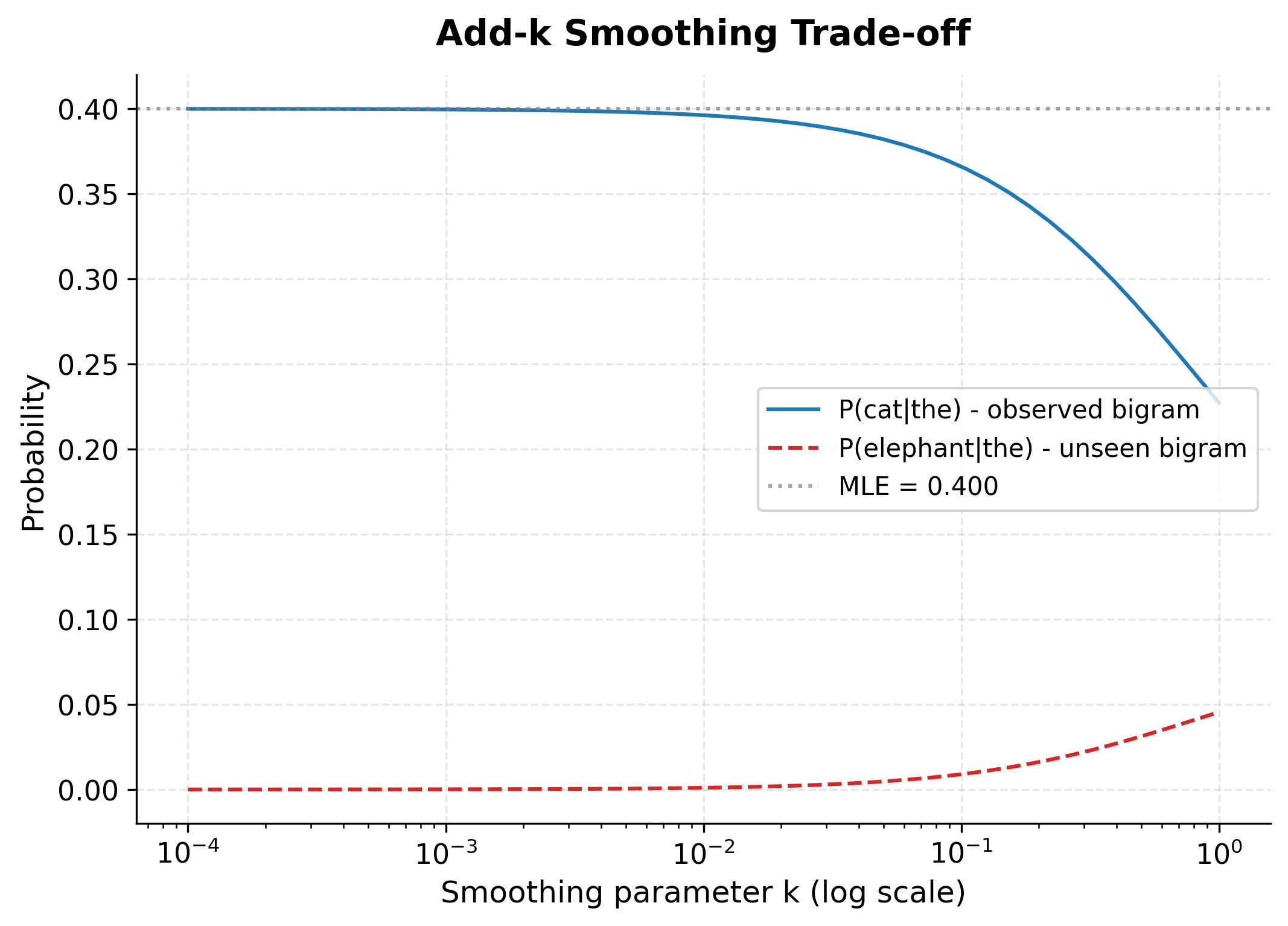
The plot reveals the fundamental trade-off. As $k$ increases, the blue curve (observed bigram) falls while the red curve (unseen bigram) rises. The gray dotted line shows the MLE estimate we're trying to preserve for observed events. Choosing $k$ means finding the right balance: small enough to keep observed probabilities reasonable, large enough to give unseen events meaningful coverage.

Good-Turing SmoothingLink Copied

Add-k smoothing has an arbitrary feel to it. Why add 0.1 rather than 0.05 or 0.2? Good-Turing smoothing takes a fundamentally different approach: instead of picking a constant, it uses the statistical structure of the data itself to determine how much probability mass should go to unseen events.

The Key Insight: Learning from SingletonsLink Copied

The core idea is elegant. If we collected more data, some n-grams that currently appear zero times would appear once. Some that appear once would appear twice. Good-Turing asks: can we use the current distribution of counts to predict this future behavior?

The answer is yes. Consider n-grams that appear exactly once in our corpus (called singletons or hapax legomena). These are the n-grams that barely made it into our observations. If we had slightly less data, many of them would have count zero. Conversely, if we had slightly more data, many currently unseen n-grams would become singletons.

This suggests that the number of singletons tells us something about unseen n-grams. More precisely: the probability mass that should go to unseen events is proportional to the number of singletons.

Frequency of Frequencies

The count $N_c$ represents how many distinct n-grams appear exactly $c$ times in the corpus. For example, $N_1$ is the number of n-grams that appear exactly once (hapax legomena), and $N_0$ is the number of n-grams that never appear.

The Good-Turing FormulaLink Copied

Good-Turing formalizes this intuition by replacing the observed count $c$ with an adjusted count $c^*$ :

c^* = (c + 1) \frac{N_{c+1}}{N_c}

The formula works by looking one step ahead in the count distribution. To estimate what a count of $c$ is really worth, we look at how many n-grams have count $c+1$ compared to how many have count $c$ . If there are relatively few n-grams with count $c+1$ , then count $c$ is probably an overestimate, and we should discount it.

For unseen n-grams (count 0), the adjusted count becomes:

0^* = \frac{N_1}{N_0}

And the total probability mass reserved for all unseen events is simply:

P_0 = \frac{N_1}{N}

where $N$ is the total number of n-gram tokens. This elegant result says: the fraction of probability mass for unseen events equals the fraction of tokens that are singletons.

Worked Example: Good-TuringLink Copied

Suppose we have a corpus with these frequency counts:

Count $c$	$N_c$ (n-grams with this count)
0	74,671,100,000
1	2,018,046
2	449,721
3	188,933
4	105,668
5	68,379

For bigrams that appear exactly once:

1^* = 2 \times \frac{449{,}721}{2{,}018{,}046} = 2 \times 0.223 = 0.446

This means a bigram seen once should be treated as if it appeared only 0.446 times. The "missing" 0.554 goes to unseen bigrams.

For unseen bigrams:

0^* = \frac{2{,}018{,}046}{74{,}671{,}100{,}000} \approx 0.000027

In[7]:

def compute_frequency_of_frequencies(counts):
    """Compute N_c: how many items have count c."""
    count_values = list(counts.values())
    freq_of_freq = Counter(count_values)
    return freq_of_freq

def good_turing_adjusted_count(c, freq_of_freq):
    """Calculate Good-Turing adjusted count c*."""
    if c == 0:
        # For unseen items, we need N_1 and total possible items
        return freq_of_freq.get(1, 0)  # Returns N_1, divide by N_0 externally
    
    N_c = freq_of_freq.get(c, 0)
    N_c_plus_1 = freq_of_freq.get(c + 1, 0)
    
    if N_c == 0:
        return c  # No adjustment possible
    
    c_star = (c + 1) * N_c_plus_1 / N_c
    return c_star

# Compute frequency of frequencies for our bigram counts
freq_of_freq = compute_frequency_of_frequencies(bigram_counts)

def compute_frequency_of_frequencies(counts):
    """Compute N_c: how many items have count c."""
    count_values = list(counts.values())
    freq_of_freq = Counter(count_values)
    return freq_of_freq

def good_turing_adjusted_count(c, freq_of_freq):
    """Calculate Good-Turing adjusted count c*."""
    if c == 0:
        # For unseen items, we need N_1 and total possible items
        return freq_of_freq.get(1, 0)  # Returns N_1, divide by N_0 externally
    
    N_c = freq_of_freq.get(c, 0)
    N_c_plus_1 = freq_of_freq.get(c + 1, 0)
    
    if N_c == 0:
        return c  # No adjustment possible
    
    c_star = (c + 1) * N_c_plus_1 / N_c
    return c_star

# Compute frequency of frequencies for our bigram counts
freq_of_freq = compute_frequency_of_frequencies(bigram_counts)

Out[8]:

Frequency of frequencies for bigrams:
----------------------------------------
N_1 =  14 (bigrams appearing 1 time(s))
N_2 =   3 (bigrams appearing 2 time(s))
N_4 =   2 (bigrams appearing 4 time(s))
N_5 =   1 (bigrams appearing 5 time(s))

Good-Turing adjusted counts:
----------------------------------------
c = 1 -> c* = 0.429
c = 2 -> c* = 0.000
c = 4 -> c* = 2.500

Our corpus shows a typical pattern: many bigrams appear only once (singletons), fewer appear twice, and so on. The adjusted count for singletons (c=1) drops significantly because Good-Turing uses the ratio of doubletons to singletons. When this ratio is less than 0.5, singletons get discounted heavily.

Out[9]:

Visualization

Bar chart showing number of bigrams at each count level, with a steep decline from count 1 to higher counts. — Frequency of frequencies distribution for bigrams. The steep decline from singletons to higher counts is characteristic of natural language, following Zipf's law. Good-Turing uses these ratios to estimate how much to discount each count level.

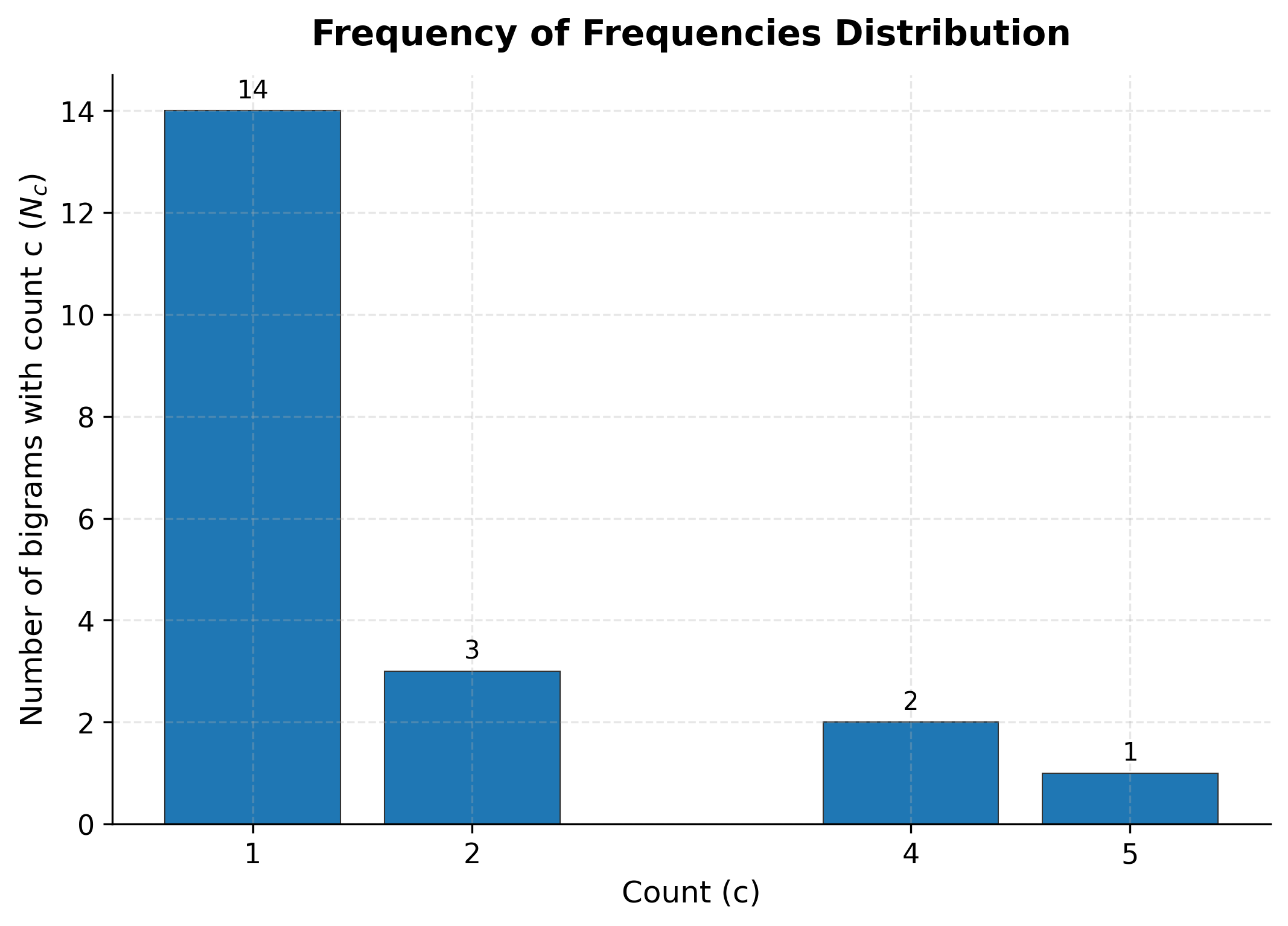
The distribution follows the expected pattern: most bigrams are rare (appearing only once or twice), while a few appear frequently. This Zipfian distribution is why Good-Turing works: the steep decline from $N_1$ to $N_2$ to $N_3$ provides the ratios needed to estimate appropriate discounts.

Good-Turing works well for small counts but becomes unreliable for larger counts where $N_c$ values become sparse or zero. In practice, it's often combined with other techniques.

Backoff and InterpolationLink Copied

Instead of modifying counts, we can use information from lower-order n-grams when higher-order ones are unreliable. Two strategies exist:

Backoff: Use the lower-order model only when the higher-order count is zero. If we've never seen the trigram "the cat ate," back off to the bigram "cat ate."

Interpolation: Always combine evidence from multiple n-gram orders using weighted averaging.

InterpolationLink Copied

Linear interpolation mixes unigram, bigram, and trigram probabilities:

P_{\text{interp}}(w_3 | w_1, w_2) = \lambda_1 P(w_3) + \lambda_2 P(w_3 | w_2) + \lambda_3 P(w_3 | w_1, w_2)

where:

$\lambda_1, \lambda_2, \lambda_3$ : interpolation weights that sum to 1 ( $\lambda_1 + \lambda_2 + \lambda_3 = 1$ )
$P(w_3)$ : unigram probability
$P(w_3 | w_2)$ : bigram probability
$P(w_3 | w_1, w_2)$ : trigram probability

The weights $\lambda$ are typically learned from held-out data using the EM algorithm or grid search.

Stupid BackoffLink Copied

A simpler approach that works surprisingly well for large-scale systems is "stupid backoff." It doesn't produce true probabilities but scores that work well for ranking:

S(w_i | w_{i-n+1}^{i-1}) = \begin{cases} \frac{C(w_{i-n+1}^i)}{C(w_{i-n+1}^{i-1})} & \text{if } C(w_{i-n+1}^i) > 0 \\ \alpha \cdot S(w_i | w_{i-n+2}^{i-1}) & \text{otherwise} \end{cases}

where:

$S(w_i | w_{i-n+1}^{i-1})$ : score for word $w_i$ given the preceding $n-1$ words
$C(w_{i-n+1}^i)$ : count of the full n-gram
$\alpha$ : backoff weight (typically 0.4)

Google used this for their web-scale language models because it's fast and the scores work well for ranking despite not being proper probabilities.

In[10]:

def interpolated_probability(trigram, lambda_weights, 
                              trigram_counts, bigram_counts, unigram_counts, 
                              total_unigrams):
    """Calculate interpolated trigram probability."""
    w1, w2, w3 = trigram
    lambda1, lambda2, lambda3 = lambda_weights
    
    # Unigram probability
    p_unigram = unigram_counts.get(w3, 0) / total_unigrams
    
    # Bigram probability
    bigram_context_count = unigram_counts.get(w2, 0)
    if bigram_context_count > 0:
        p_bigram = bigram_counts.get((w2, w3), 0) / bigram_context_count
    else:
        p_bigram = 0
    
    # Trigram probability
    trigram_context = bigram_counts.get((w1, w2), 0)
    if trigram_context > 0:
        p_trigram = trigram_counts.get(trigram, 0) / trigram_context
    else:
        p_trigram = 0
    
    return lambda1 * p_unigram + lambda2 * p_bigram + lambda3 * p_trigram

# Build trigram counts
def get_trigrams(sentences):
    trigrams = []
    for sentence in sentences:
        tokens = ["<s>", "<s>"] + sentence.lower().split() + ["</s>"]
        for i in range(len(tokens) - 2):
            trigrams.append((tokens[i], tokens[i + 1], tokens[i + 2]))
    return trigrams

trigrams = get_trigrams(corpus)
trigram_counts = Counter(trigrams)
total_unigrams = sum(unigram_counts.values())

# Test interpolation with different weight combinations
lambda_sets = [
    (0.1, 0.3, 0.6),  # Favor trigrams
    (0.2, 0.4, 0.4),  # Balanced
    (0.5, 0.3, 0.2),  # Favor unigrams
]

def interpolated_probability(trigram, lambda_weights, 
                              trigram_counts, bigram_counts, unigram_counts, 
                              total_unigrams):
    """Calculate interpolated trigram probability."""
    w1, w2, w3 = trigram
    lambda1, lambda2, lambda3 = lambda_weights
    
    # Unigram probability
    p_unigram = unigram_counts.get(w3, 0) / total_unigrams
    
    # Bigram probability
    bigram_context_count = unigram_counts.get(w2, 0)
    if bigram_context_count > 0:
        p_bigram = bigram_counts.get((w2, w3), 0) / bigram_context_count
    else:
        p_bigram = 0
    
    # Trigram probability
    trigram_context = bigram_counts.get((w1, w2), 0)
    if trigram_context > 0:
        p_trigram = trigram_counts.get(trigram, 0) / trigram_context
    else:
        p_trigram = 0
    
    return lambda1 * p_unigram + lambda2 * p_bigram + lambda3 * p_trigram

# Build trigram counts
def get_trigrams(sentences):
    trigrams = []
    for sentence in sentences:
        tokens = ["<s>", "<s>"] + sentence.lower().split() + ["</s>"]
        for i in range(len(tokens) - 2):
            trigrams.append((tokens[i], tokens[i + 1], tokens[i + 2]))
    return trigrams

trigrams = get_trigrams(corpus)
trigram_counts = Counter(trigrams)
total_unigrams = sum(unigram_counts.values())

# Test interpolation with different weight combinations
lambda_sets = [
    (0.1, 0.3, 0.6),  # Favor trigrams
    (0.2, 0.4, 0.4),  # Balanced
    (0.5, 0.3, 0.2),  # Favor unigrams
]

Out[11]:

Testing trigram: ('<s>', 'the', 'cat')
Trigram count: 3
Bigram count ('<s>', 'the'): 5

λ = (0.1, 0.3, 0.6): P(cat|<s>,the) = 0.492121
λ = (0.2, 0.4, 0.4): P(cat|<s>,the) = 0.424242
λ = (0.5, 0.3, 0.2): P(cat|<s>,the) = 0.300606

The weight distribution matters. When we favor trigrams ( $\lambda_3 = 0.6$ ), the probability is higher because the trigram "<s> the cat" appears in our corpus. When we favor unigrams ( $\lambda_1 = 0.5$ ), we rely more on how often "cat" appears overall, which dilutes the context-specific information.

Interpolation provides a smooth fallback mechanism. Even when the trigram count is zero, the bigram and unigram components contribute to a non-zero probability.

Kneser-Ney SmoothingLink Copied

The smoothing methods we've seen so far share a common limitation: they treat the backoff distribution as a simple unigram model based on word frequency. But word frequency alone can be misleading. Kneser-Ney smoothing addresses this with two innovations that, together, create the most effective n-gram smoothing method ever developed.

The Problem with Frequency-Based BackoffLink Copied

To understand why Kneser-Ney matters, consider the phrase "San Francisco." In any corpus about California, the word "Francisco" appears frequently. A standard unigram model would assign it high probability.

But here's the catch: "Francisco" almost always follows "San." It rarely appears in other contexts. If we're backing off from an unseen trigram like "visited beautiful Francisco," a frequency-based unigram model would say "Francisco" is likely. Yet intuitively, we know "Francisco" is an unlikely word to appear after "beautiful" because it almost never starts a new context on its own.

This observation leads to Kneser-Ney's key insight: when backing off, we shouldn't ask "how often does this word appear?" but rather "in how many different contexts does this word appear?"

Innovation 1: Absolute DiscountingLink Copied

The first innovation is straightforward. Instead of using Good-Turing's complex count adjustments, Kneser-Ney subtracts a fixed discount $d$ from every observed count:

P_{\text{abs}}(w_i | w_{i-1}) = \frac{\max(C(w_{i-1}, w_i) - d, 0)}{C(w_{i-1})} + \lambda(w_{i-1}) P_{\text{lower}}(w_i)

The formula has two terms:

Discounted probability: The observed count minus $d$ , divided by the context count. The $\max$ ensures we never go negative.
Backoff contribution: An interpolation weight $\lambda$ times a lower-order probability.

The discount $d$ is typically 0.75, a value derived from theoretical analysis of Good-Turing estimates. By subtracting a fixed amount rather than a percentage, absolute discounting treats all observed n-grams more uniformly. An n-gram seen 5 times loses 0.75 (15%), while one seen 2 times loses 0.75 (37.5%). This makes sense: rare observations are less reliable and should be discounted more aggressively in relative terms.

Innovation 2: Continuation ProbabilityLink Copied

The second innovation is where Kneser-Ney truly shines. For the backoff distribution $P_{\text{lower}}$ , it doesn't use raw word frequency. Instead, it uses continuation probability: the proportion of unique contexts in which a word appears.

P_{\text{continuation}}(w) = \frac{|\{w_{i-1} : C(w_{i-1}, w) > 0\}|}{|\{(w_{i-1}, w_i) : C(w_{i-1}, w_i) > 0\}|}

Let's unpack this:

Numerator: Count how many unique words precede $w$ . For "Francisco," this might be just 1 (only "San" precedes it). For "the," it might be hundreds.
Denominator: The total number of unique bigram types in the corpus.

Returning to our example: "Francisco" has high frequency but low continuation count (appears after few unique words). "The" has high frequency and high continuation count (appears after many unique words). When backing off, "the" deserves higher probability than "Francisco" because it's a more versatile word that genuinely appears in diverse contexts.

Putting It Together: The Full FormulaLink Copied

The complete Kneser-Ney formula for the highest-order n-gram combines both innovations:

P_{\text{KN}}(w_i | w_{i-n+1}^{i-1}) = \frac{\max(C(w_{i-n+1}^i) - d, 0)}{C(w_{i-n+1}^{i-1})} + \lambda(w_{i-n+1}^{i-1}) P_{\text{KN}}(w_i | w_{i-n+2}^{i-1})

where:

$w_{i-n+1}^{i-1}$ : the context (preceding $n-1$ words)
$C(w_{i-n+1}^i)$ : count of the full n-gram
$d$ : discount value (typically 0.75)

The interpolation weight $\lambda$ ensures probability mass is conserved. It equals the total amount discounted from all observed continuations:

\lambda(w_{i-n+1}^{i-1}) = \frac{d}{C(w_{i-n+1}^{i-1})} \times |\{w : C(w_{i-n+1}^{i-1}, w) > 0\}|

This formula says: take the discount $d$ , multiply by the number of unique words that follow this context, and divide by the total context count. The result is exactly the probability mass we "stole" from observed n-grams, which we now redistribute through the backoff distribution.

For lower-order distributions (used in the recursive backoff), raw counts are replaced with continuation counts. This is what makes the "San Francisco" example work correctly: "Francisco" has low continuation count, so it receives low probability in the backoff distribution despite its high raw frequency.

In[12]:

def kneser_ney_bigram(bigram, d, bigram_counts, unigram_counts, 
                      continuation_counts, total_bigram_types):
    """Calculate Kneser-Ney smoothed bigram probability."""
    w1, w2 = bigram
    
    # Count of this bigram
    bigram_count = bigram_counts.get(bigram, 0)
    context_count = unigram_counts.get(w1, 0)
    
    if context_count == 0:
        # Fall back to continuation probability only
        return continuation_counts.get(w2, 0) / total_bigram_types
    
    # First term: discounted probability
    first_term = max(bigram_count - d, 0) / context_count
    
    # Lambda: interpolation weight
    unique_continuations = sum(1 for (w1_prime, w2_prime) in bigram_counts 
                               if w1_prime == w1)
    lambda_weight = (d / context_count) * unique_continuations
    
    # Continuation probability for w2
    p_continuation = continuation_counts.get(w2, 0) / total_bigram_types
    
    return first_term + lambda_weight * p_continuation

# Compute continuation counts: how many unique contexts precede each word
continuation_counts = Counter()
for (w1, w2) in bigram_counts:
    continuation_counts[w2] += 1

total_bigram_types = len(bigram_counts)
d = 0.75  # Standard discount value

def kneser_ney_bigram(bigram, d, bigram_counts, unigram_counts, 
                      continuation_counts, total_bigram_types):
    """Calculate Kneser-Ney smoothed bigram probability."""
    w1, w2 = bigram
    
    # Count of this bigram
    bigram_count = bigram_counts.get(bigram, 0)
    context_count = unigram_counts.get(w1, 0)
    
    if context_count == 0:
        # Fall back to continuation probability only
        return continuation_counts.get(w2, 0) / total_bigram_types
    
    # First term: discounted probability
    first_term = max(bigram_count - d, 0) / context_count
    
    # Lambda: interpolation weight
    unique_continuations = sum(1 for (w1_prime, w2_prime) in bigram_counts 
                               if w1_prime == w1)
    lambda_weight = (d / context_count) * unique_continuations
    
    # Continuation probability for w2
    p_continuation = continuation_counts.get(w2, 0) / total_bigram_types
    
    return first_term + lambda_weight * p_continuation

# Compute continuation counts: how many unique contexts precede each word
continuation_counts = Counter()
for (w1, w2) in bigram_counts:
    continuation_counts[w2] += 1

total_bigram_types = len(bigram_counts)
d = 0.75  # Standard discount value

Out[13]:

Continuation counts (unique preceding contexts):
--------------------------------------------------
  '</s>': appears after 5 unique word(s)
  'the': appears after 4 unique word(s)
  'sat': appears after 2 unique word(s)
  'chased': appears after 2 unique word(s)
  'cat': appears after 1 unique word(s)
  'on': appears after 1 unique word(s)
  'mat': appears after 1 unique word(s)
  'dog': appears after 1 unique word(s)

Total unique bigram types: 20

Kneser-Ney probabilities (d = 0.75):
--------------------------------------------------
P(cat|the): 0.340000  (raw count: 4)
P(dog|the): 0.340000  (raw count: 4)
P(sat|cat): 0.137500  (raw count: 1)
P(elephant|the): 0.000000  (raw count: 0)

The continuation counts reveal which words are versatile. Words like "the" and "cat" appear after multiple different words, giving them higher continuation probability. The word "" (end of sentence) also has high continuation count because every sentence ends with it.

Out[14]:

Visualization

Scatter plot comparing continuation count to raw frequency for each word, with a diagonal reference line. — Continuation count vs raw frequency for each word. Words above the diagonal appear in more unique contexts than their frequency alone would suggest (versatile words). Words below appear in fewer contexts (context-dependent words like 'Francisco' would be).

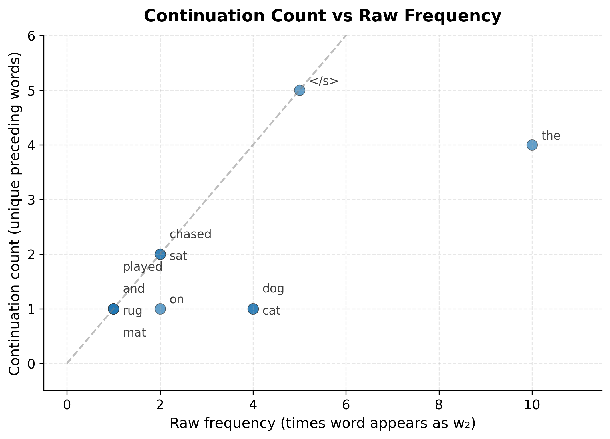
The scatter plot illustrates Kneser-Ney's key insight. Words near or above the diagonal line are "versatile," appearing in many different contexts relative to their frequency. Words below the line are context-dependent, appearing frequently but in limited contexts. In a larger corpus, "Francisco" would appear far below the diagonal (high frequency, low continuation count), while common function words like "the" would appear on or above it.

Kneser-Ney assigns non-zero probability to the unseen bigram "the elephant" through the continuation probability term, while keeping observed bigrams at reasonable levels. The discount of 0.75 is subtracted from each observed count, and the freed probability mass flows to the continuation distribution.

Modified Kneser-NeyLink Copied

Modified Kneser-Ney improves on the original by using three different discount values based on the count:

d(c) = \begin{cases} d_1 & \text{if } c = 1 \\ d_2 & \text{if } c = 2 \\ d_3 & \text{if } c \geq 3 \end{cases}

These are estimated from the training data:

d_1 = 1 - 2Y\frac{N_2}{N_1}, \quad d_2 = 2 - 3Y\frac{N_3}{N_2}, \quad d_3 = 3 - 4Y\frac{N_4}{N_3}

where:

$Y = \frac{N_1}{N_1 + 2N_2}$ : a normalization factor based on singleton and doubleton counts
$N_c$ : number of n-grams appearing exactly $c$ times

The intuition is that n-grams seen once are more likely to be noise than those seen twice, which are more likely to be noise than those seen three or more times. Different discounts capture this.

In[15]:

def compute_modified_kn_discounts(freq_of_freq):
    """Compute the three discount values for Modified Kneser-Ney."""
    N1 = freq_of_freq.get(1, 1)
    N2 = freq_of_freq.get(2, 1)
    N3 = freq_of_freq.get(3, 1)
    N4 = freq_of_freq.get(4, 1)
    
    # Avoid division by zero
    if N1 + 2 * N2 == 0:
        Y = 0
    else:
        Y = N1 / (N1 + 2 * N2)
    
    d1 = 1 - 2 * Y * (N2 / N1) if N1 > 0 else 0
    d2 = 2 - 3 * Y * (N3 / N2) if N2 > 0 else 0
    d3 = 3 - 4 * Y * (N4 / N3) if N3 > 0 else 0
    
    # Clamp to reasonable range
    d1 = max(0, min(1, d1))
    d2 = max(0, min(2, d2))
    d3 = max(0, min(3, d3))
    
    return d1, d2, d3, Y

d1, d2, d3, Y = compute_modified_kn_discounts(freq_of_freq)

def compute_modified_kn_discounts(freq_of_freq):
    """Compute the three discount values for Modified Kneser-Ney."""
    N1 = freq_of_freq.get(1, 1)
    N2 = freq_of_freq.get(2, 1)
    N3 = freq_of_freq.get(3, 1)
    N4 = freq_of_freq.get(4, 1)
    
    # Avoid division by zero
    if N1 + 2 * N2 == 0:
        Y = 0
    else:
        Y = N1 / (N1 + 2 * N2)
    
    d1 = 1 - 2 * Y * (N2 / N1) if N1 > 0 else 0
    d2 = 2 - 3 * Y * (N3 / N2) if N2 > 0 else 0
    d3 = 3 - 4 * Y * (N4 / N3) if N3 > 0 else 0
    
    # Clamp to reasonable range
    d1 = max(0, min(1, d1))
    d2 = max(0, min(2, d2))
    d3 = max(0, min(3, d3))
    
    return d1, d2, d3, Y

d1, d2, d3, Y = compute_modified_kn_discounts(freq_of_freq)

Out[16]:

Modified Kneser-Ney discount parameters:
----------------------------------------
Y = 0.7000
d1 (for count=1): 0.7000
d2 (for count=2): 1.3000
d3 (for count≥3): 0.0000

The Y factor normalizes based on the ratio of singletons to doubletons. With our small corpus, the discount values are at their boundary conditions. On larger corpora, typical values are around $d_1 \approx 0.7$ , $d_2 \approx 1.0$ , and $d_3 \approx 1.3$ . The progression makes intuitive sense: we discount singletons more aggressively because they're more likely to be noise, while n-grams seen three or more times are more reliable and get smaller relative discounts.

Comparing Smoothing MethodsLink Copied

Let's compare how different smoothing methods handle the same probability estimation task.

In[17]:

import matplotlib.pyplot as plt

def mle_probability(bigram, bigram_counts, unigram_counts):
    """Maximum likelihood estimate."""
    w1, w2 = bigram
    context = unigram_counts.get(w1, 0)
    if context == 0:
        return 0
    return bigram_counts.get(bigram, 0) / context

# Collect probabilities for all methods
methods = ["MLE", "Add-1", "Add-0.1", "Add-0.01", "Kneser-Ney"]
test_words = ["cat", "dog", "sat", "on", "mat", "elephant", "zebra"]

# Create test bigrams with "the" as context
results = {method: [] for method in methods}

for word in test_words:
    bigram = ("the", word)
    
    # MLE
    results["MLE"].append(mle_probability(bigram, bigram_counts, unigram_counts))
    
    # Add-k variants
    results["Add-1"].append(add_k_probability(bigram, 1.0, bigram_counts, unigram_counts, V))
    results["Add-0.1"].append(add_k_probability(bigram, 0.1, bigram_counts, unigram_counts, V))
    results["Add-0.01"].append(add_k_probability(bigram, 0.01, bigram_counts, unigram_counts, V))
    
    # Kneser-Ney
    results["Kneser-Ney"].append(kneser_ney_bigram(bigram, 0.75, bigram_counts, 
                                                    unigram_counts, continuation_counts, 
                                                    total_bigram_types))

import matplotlib.pyplot as plt

def mle_probability(bigram, bigram_counts, unigram_counts):
    """Maximum likelihood estimate."""
    w1, w2 = bigram
    context = unigram_counts.get(w1, 0)
    if context == 0:
        return 0
    return bigram_counts.get(bigram, 0) / context

# Collect probabilities for all methods
methods = ["MLE", "Add-1", "Add-0.1", "Add-0.01", "Kneser-Ney"]
test_words = ["cat", "dog", "sat", "on", "mat", "elephant", "zebra"]

# Create test bigrams with "the" as context
results = {method: [] for method in methods}

for word in test_words:
    bigram = ("the", word)
    
    # MLE
    results["MLE"].append(mle_probability(bigram, bigram_counts, unigram_counts))
    
    # Add-k variants
    results["Add-1"].append(add_k_probability(bigram, 1.0, bigram_counts, unigram_counts, V))
    results["Add-0.1"].append(add_k_probability(bigram, 0.1, bigram_counts, unigram_counts, V))
    results["Add-0.01"].append(add_k_probability(bigram, 0.01, bigram_counts, unigram_counts, V))
    
    # Kneser-Ney
    results["Kneser-Ney"].append(kneser_ney_bigram(bigram, 0.75, bigram_counts, 
                                                    unigram_counts, continuation_counts, 
                                                    total_bigram_types))

Out[18]:

Visualization

Bar chart comparing five smoothing methods across seven words, showing MLE with zeros for unseen words and smoothing methods with non-zero estimates. — Comparison of probability estimates across smoothing methods. MLE assigns zero to unseen words, while smoothing methods redistribute probability mass. Kneser-Ney maintains higher probabilities for observed words while still covering unseen ones.

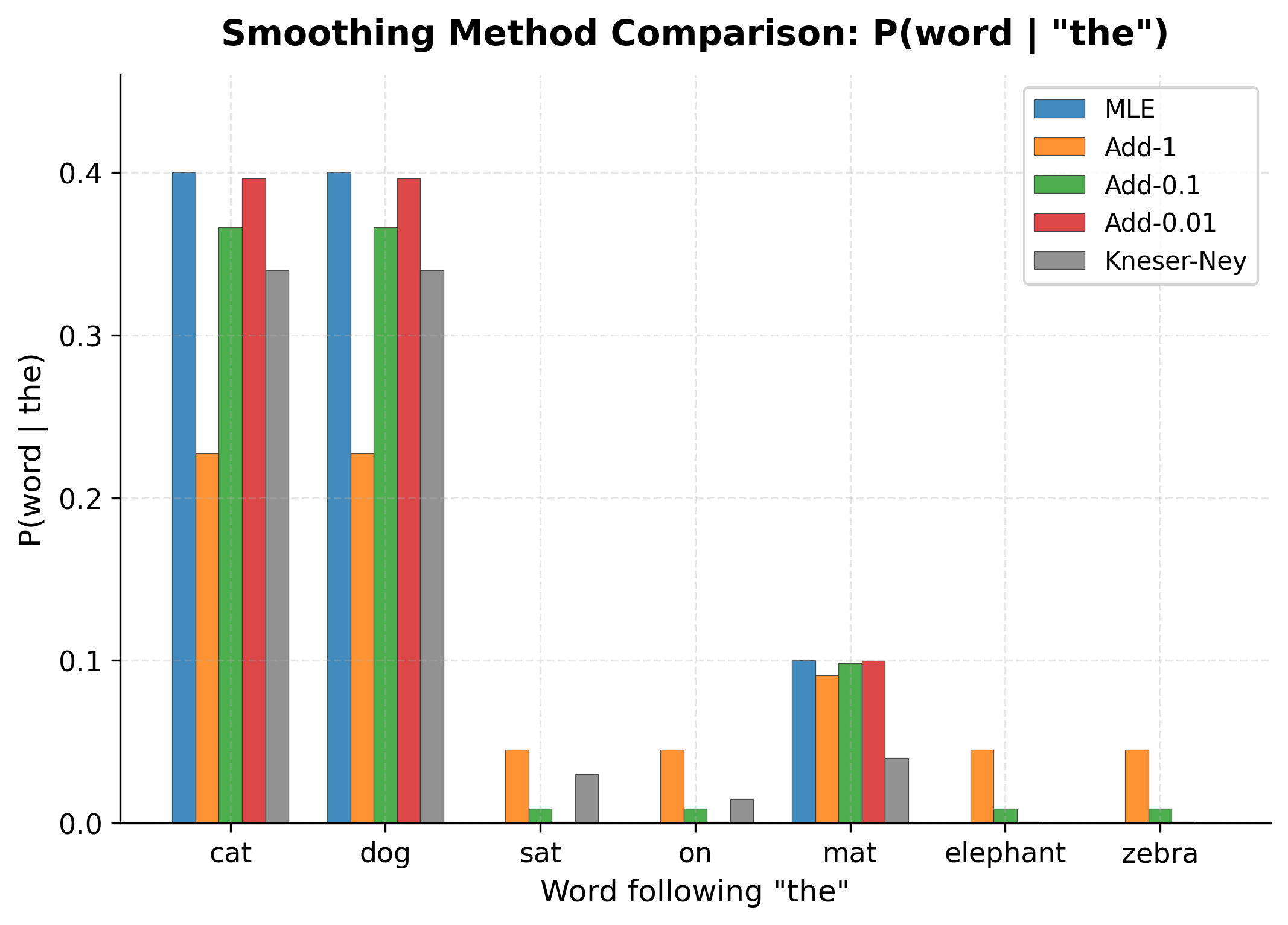
The chart reveals the trade-offs clearly. MLE gives the highest probabilities to observed words but zeros for unseen ones. Add-1 smoothing flattens everything too much. Add-0.01 and Kneser-Ney strike a better balance, keeping observed words relatively high while providing coverage for unseen words.

Out[19]:

Probability estimates for P(word|the):
===========================================================================
Word                MLE      Add-1    Add-0.1   Add-0.01         KN
---------------------------------------------------------------------------
cat            0.400000   0.227273   0.366071   0.396245   0.340000
dog            0.400000   0.227273   0.366071   0.396245   0.340000
sat            0.000000   0.045455   0.008929   0.000988   0.030000
on             0.000000   0.045455   0.008929   0.000988   0.015000
mat            0.100000   0.090909   0.098214   0.099802   0.040000
elephant       0.000000   0.045455   0.008929   0.000988   0.000000
zebra          0.000000   0.045455   0.008929   0.000988   0.000000

The table quantifies what we saw in the chart. For observed words like "cat" and "dog," MLE gives the highest probability, but Add-1 drops it dramatically. Kneser-Ney maintains probabilities closer to MLE for observed words while still providing coverage for unseen ones like "elephant" and "zebra." This balance is why Kneser-Ney became the standard for production language models.

Limitations and ImpactLink Copied

LimitationsLink Copied

Smoothing techniques, despite their sophistication, have inherent limitations:

Fixed context window: All n-gram smoothing methods are bounded by the Markov assumption. No amount of smoothing helps when the relevant context is beyond the n-gram window.
Vocabulary dependence: Performance degrades with vocabulary size. As $V$ grows, the number of possible unseen n-grams explodes.
Domain sensitivity: Smoothing parameters tuned on one domain may perform poorly on another. A model trained on news text with optimal smoothing for that domain may still struggle with social media text.
No semantic awareness: Smoothing treats "the cat ate" and "the cat flew" identically if both are unseen. It cannot use semantic knowledge that cats are more likely to eat than fly.

ImpactLink Copied

Despite these limitations, smoothing techniques were foundational to practical NLP:

Speech recognition: Kneser-Ney smoothing powered speech recognition systems for decades, enabling reliable transcription even for novel word combinations.
Machine translation: Statistical MT systems relied heavily on smoothed language models to score translation candidates.
Spell correction: Smoothed models help distinguish between plausible and implausible word sequences for context-aware spelling correction.
Established evaluation practices: The development of smoothing techniques led to rigorous evaluation methods like perplexity comparison on held-out data.

The techniques in this chapter represent the pinnacle of count-based language modeling. They squeezed remarkable performance from simple statistics. But they also revealed the ceiling: no matter how clever the smoothing, n-gram models cannot capture long-range dependencies or semantic similarity. This limitation motivated the shift to neural language models, which learn continuous representations that naturally generalize to unseen word combinations.

SummaryLink Copied

Smoothing techniques solve the zero probability problem in n-gram language models by redistributing probability mass from observed to unseen events.

Key takeaways:

Laplace (add-one) smoothing is simple but steals too much probability from observed events
Add-k smoothing improves by using smaller constants, with $k$ tuned on held-out data
Good-Turing smoothing uses frequency of frequencies to estimate probability mass for unseen events
Interpolation combines evidence from multiple n-gram orders using learned weights
Kneser-Ney smoothing uses absolute discounting and continuation probability, making it the gold standard for n-gram models
Modified Kneser-Ney refines discounting with count-dependent values

The choice of smoothing method matters significantly. On large corpora, Kneser-Ney typically outperforms simpler methods by 10-20% in perplexity. For small corpora or quick experiments, add-k smoothing provides a reasonable baseline with minimal implementation effort.

These techniques represent the culmination of decades of statistical NLP research. While neural language models have largely superseded n-gram models for most applications, understanding smoothing provides essential intuition about probability estimation, the bias-variance trade-off, and the importance of handling unseen events, concepts that remain central to modern NLP.

Key ParametersLink Copied

When implementing smoothing techniques, these parameters have the most impact on model performance:

Parameter	Typical Range	Effect
$k$ (add-k smoothing)	0.001 - 0.5	Controls probability mass given to unseen events. Smaller values stay closer to MLE; larger values flatten the distribution. Tune on held-out data.
$d$ (Kneser-Ney discount)	0.75	Fixed discount subtracted from all counts. The standard value of 0.75 works well across most corpora.
$d_1, d_2, d_3$ (Modified KN)	0.7, 1.0, 1.3	Count-dependent discounts. Computed from corpus statistics using the formulas above. No manual tuning needed.
$\lambda$ weights (interpolation)	Sum to 1.0	Control contribution of each n-gram order. Learn from held-out data using EM or grid search. Higher-order weights should generally be larger.
$\alpha$ (stupid backoff)	0.4	Backoff penalty applied when falling back to lower-order n-grams. The value 0.4 was empirically determined by Google.
$n$ (n-gram order)	3 - 5	Higher orders capture more context but suffer more from sparsity. Trigrams are common; 5-grams require very large corpora.

QuizLink Copied

Ready to test your understanding? Take this quick quiz to reinforce what you've learned about smoothing techniques for n-gram language models.

Loading component...

Back to Language AI Handbook

Previous Chapter

N-gram Language Models

Next Chapter

Perplexity

Coming Soon

Reference

BIBTEXAcademic

@misc{smoothingtechniquesforngramlanguagemodelsfromlaplacetokneserney, author = {Michael Brenndoerfer}, title = {Smoothing Techniques for N-gram Language Models: From Laplace to Kneser-Ney}, year = {2025}, url = {https://mbrenndoerfer.com/writing/smoothing-techniques-ngram-language-models-laplace-kneser-ney}, organization = {mbrenndoerfer.com}, note = {Accessed: 2025-12-07} }

APAAcademic

Michael Brenndoerfer (2025). Smoothing Techniques for N-gram Language Models: From Laplace to Kneser-Ney. Retrieved from https://mbrenndoerfer.com/writing/smoothing-techniques-ngram-language-models-laplace-kneser-ney

MLAAcademic

Michael Brenndoerfer. "Smoothing Techniques for N-gram Language Models: From Laplace to Kneser-Ney." 2025. Web. 12/7/2025. <https://mbrenndoerfer.com/writing/smoothing-techniques-ngram-language-models-laplace-kneser-ney>.

CHICAGOAcademic

Michael Brenndoerfer. "Smoothing Techniques for N-gram Language Models: From Laplace to Kneser-Ney." Accessed 12/7/2025. https://mbrenndoerfer.com/writing/smoothing-techniques-ngram-language-models-laplace-kneser-ney.

HARVARDAcademic

Michael Brenndoerfer (2025) 'Smoothing Techniques for N-gram Language Models: From Laplace to Kneser-Ney'. Available at: https://mbrenndoerfer.com/writing/smoothing-techniques-ngram-language-models-laplace-kneser-ney (Accessed: 12/7/2025).

SimpleBasic

Michael Brenndoerfer (2025). Smoothing Techniques for N-gram Language Models: From Laplace to Kneser-Ney. https://mbrenndoerfer.com/writing/smoothing-techniques-ngram-language-models-laplace-kneser-ney

Direct link:

https://mbrenndoerfer.com/writing/smoothing-techniques-ngram-language-models-laplace-kneser-ney

Part of Language AI Handbook

This article is part of the free-to-read Language AI Handbook

About the author: Michael Brenndoerfer

All opinions expressed here are my own and do not reflect the views of my employer.

Michael currently works as an Associate Director of Data Science at EQT Partners in Singapore, where he drives AI and data initiatives across private capital investments.

With over a decade of experience spanning private equity, management consulting, and software engineering, he specializes in building and scaling analytics capabilities from the ground up. He has published research in leading AI conferences and holds expertise in machine learning, natural language processing, and value creation through data.

View Full Resume Publications Contact Books

InteractiveSmoothing Techniques for N-gram Language Models: From Laplace to Kneser-Ney

Smoothing TechniquesLink Copied

The Zero Probability ProblemLink Copied

Add-One (Laplace) SmoothingLink Copied

Worked Example: Laplace SmoothingLink Copied

Add-k SmoothingLink Copied

Tuning kLink Copied

Good-Turing SmoothingLink Copied

The Key Insight: Learning from SingletonsLink Copied

The Good-Turing FormulaLink Copied

Worked Example: Good-TuringLink Copied

Backoff and InterpolationLink Copied

InterpolationLink Copied

Stupid BackoffLink Copied

Kneser-Ney SmoothingLink Copied

The Problem with Frequency-Based BackoffLink Copied

Innovation 1: Absolute DiscountingLink Copied

Innovation 2: Continuation ProbabilityLink Copied

Putting It Together: The Full FormulaLink Copied

Modified Kneser-NeyLink Copied

Comparing Smoothing MethodsLink Copied

Limitations and ImpactLink Copied

LimitationsLink Copied

ImpactLink Copied

SummaryLink Copied

Key ParametersLink Copied

QuizLink Copied

Reference

About the author: Michael Brenndoerfer

Related Content

N-gram Language Models: Probability-Based Text Generation & Prediction

Bag of Words: Document-Term Matrices, Vocabulary Construction & Sparse Representations

N-grams: Capturing Word Order in Text with Bigrams, Trigrams & Skip-grams

Stay updated