

Learn how the Bag of Words model transforms text into numerical vectors through word counting, vocabulary construction, and sparse matrix storage. Master CountVectorizer and understand when this foundational NLP technique works best.

This article is part of the free-to-read Language AI Handbook
Choose your expertise level to adjust how many terms are explained. Beginners see more tooltips, experts see fewer to maintain reading flow. Hover over underlined terms for instant definitions.
Bag of Words
How do you teach a computer to understand text? The first step is deceptively simple: count words. The Bag of Words (BoW) model transforms documents into numerical vectors by tallying how often each word appears. This representation ignores grammar, word order, and context entirely. It treats a document as nothing more than a collection of words tossed into a bag, hence the name.
Despite its simplicity, Bag of Words powered text classification, spam detection, and information retrieval for decades. It remains a surprisingly effective baseline for many NLP tasks. Understanding BoW is essential because it introduces core concepts (vocabulary construction, document-term matrices, and sparse representations) that persist throughout modern NLP.
This chapter walks you through building a Bag of Words representation from scratch. You'll learn how to construct vocabularies, create document-term matrices, handle the explosion of dimensionality with sparse matrices, and understand when this simple approach works and when it fails.
The Core Idea
Consider three short documents:
- "The cat sat on the mat"
- "The dog sat on the log"
- "The cat and the dog"
To represent these numerically, we first build a vocabulary: a list of all unique words across all documents. Then we count how many times each vocabulary word appears in each document.
The Bag of Words model represents text as an unordered collection of words, disregarding grammar and word order but keeping track of word frequency. Each document becomes a vector where each dimension corresponds to a vocabulary word, and the value indicates how often that word appears.
Let's implement this step by step:
The vocabulary contains all unique words found across the documents. Each word maps to a unique index that will become a dimension in our vector representation.
Each row represents a document, and each column represents a word from our vocabulary. Formally, we can express the document-term matrix as where element represents the count of vocabulary word in document . Here, is the number of documents and is the vocabulary size.
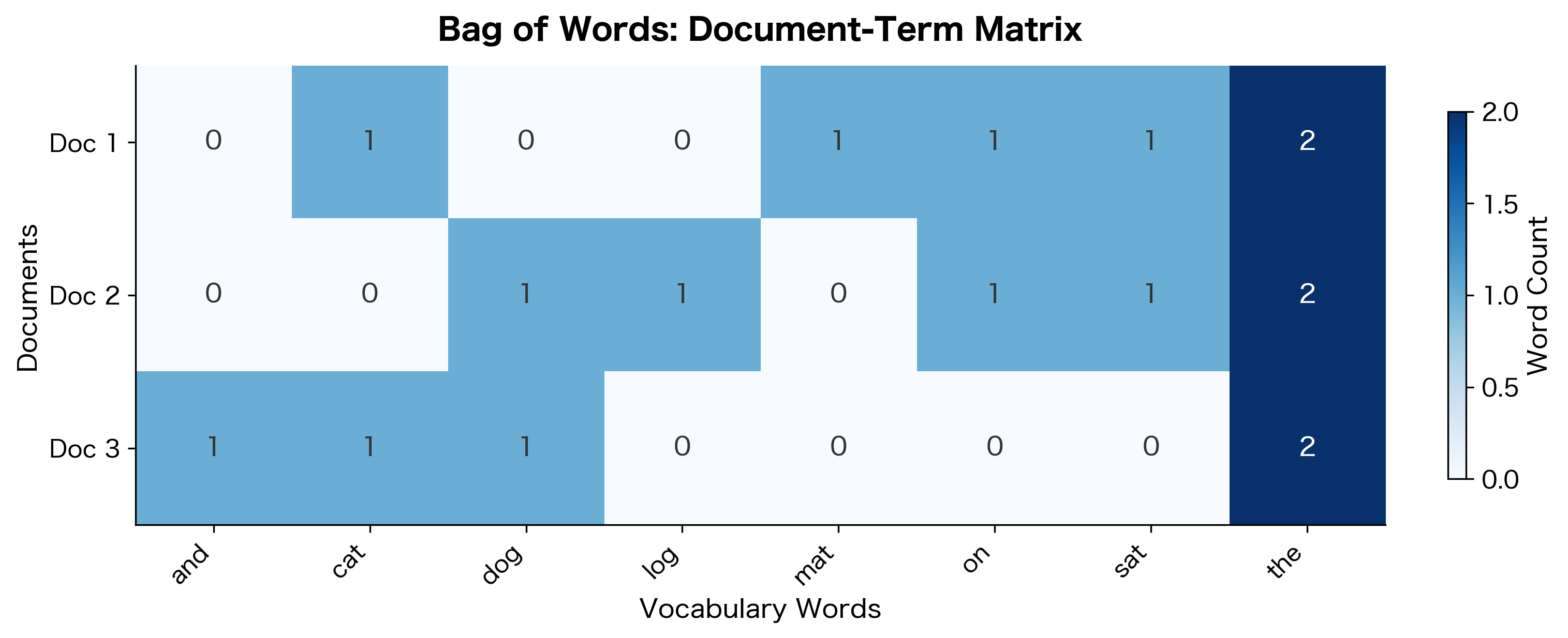
Look at the matrix structure. Document 1 has two occurrences of "the" (the cat... the mat), reflected in the count of 2. Document 3 shares vocabulary with both other documents, which we can see from the overlapping non-zero entries.
Document Similarity from Word Counts
Once documents become vectors, we can measure their similarity using cosine similarity. This metric computes the cosine of the angle between two vectors, effectively measuring how similar their directions are in high-dimensional space, regardless of their magnitudes.
Given two document vectors and , cosine similarity is defined as:
where:
- : the dot product of vectors and , computed as
- : the Euclidean norm (magnitude) of vector , computed as
- : the vocabulary size (number of dimensions in each vector)
- : the word counts at position in vectors and respectively
The result ranges from 0 (completely different, no shared vocabulary) to 1 (identical word distributions). By normalizing by vector magnitudes, cosine similarity ensures that documents with similar word proportions are considered similar even if one document is much longer than the other.
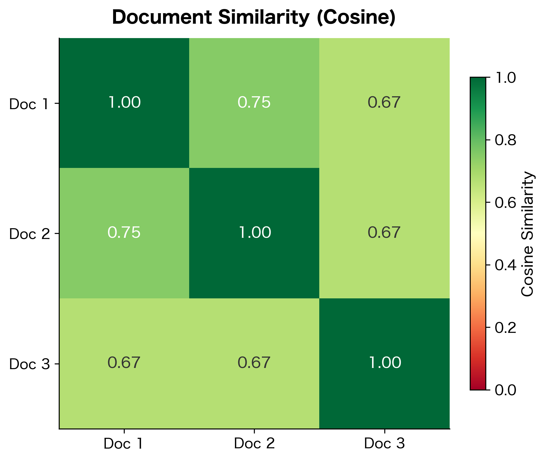
Documents 1 and 2 are most similar because they share the phrase structure "The [animal] sat on the [object]". Document 3, with its different structure, shows lower similarity to both. This demonstrates how BoW captures topical similarity through shared vocabulary, even though it ignores word order.
Vocabulary Construction
Building a vocabulary seems straightforward, but real-world text introduces complications. How do you handle punctuation? What about rare words that appear only once? What about extremely common words like "the" that appear everywhere?
From Corpus to Vocabulary
A corpus is a collection of documents. The vocabulary is the set of unique terms extracted from this corpus. Let's work with a slightly more realistic example:
The vocabulary is significantly smaller than the total token count because many words repeat across documents. This compression—from raw tokens to unique vocabulary terms—is a key characteristic of text data.
Word Frequency Analysis
Before finalizing the vocabulary, examining word frequencies helps identify potential issues:
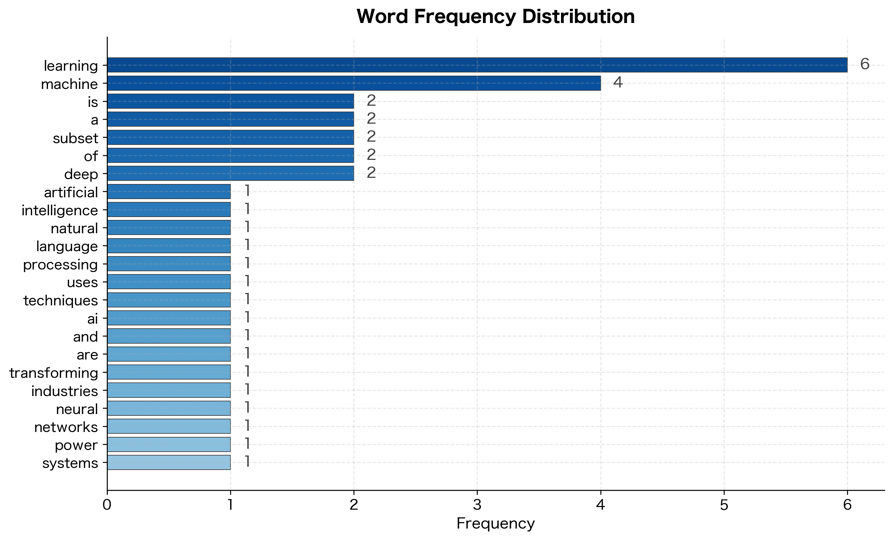
The word "learning" appears 5 times, "machine" appears 4 times, but many words appear only once. This pattern, a few high-frequency words and many rare words, follows Zipf's Law and is characteristic of natural language.
Vocabulary Pruning
Raw vocabularies from large corpora can contain millions of unique words. Many of these are noise: typos, rare technical terms, or words that appear in only one document. Vocabulary pruning removes uninformative terms to reduce dimensionality and improve model performance.
Minimum Document Frequency
The document frequency of a word , denoted , is the number of documents in which that word appears at least once:
where:
- : the corpus (collection of all documents)
- : an individual document in the corpus
- : indicates that word appears in document
- : the count of elements in the set
Words that appear in very few documents provide little discriminative power and may represent noise. The min_df parameter sets a threshold: words must appear in at least this many documents (or this fraction of documents) to be included.
Words like "artificial", "industries", and "networks" appear in only one document. Removing them reduces our vocabulary while keeping words that appear across multiple documents.
Maximum Document Frequency
At the other extreme, words that appear in almost every document provide no discriminative power. The word "the" might appear in 95% of documents, making it useless for distinguishing between them. The max_df parameter sets an upper threshold.
In our small corpus, "learning" appears in all 5 documents (100%), exceeding our 80% threshold. In real applications, you might filter out words appearing in more than 90% of documents to remove uninformative terms like "the", "is", and "a".
Vocabulary Reduction with min_df
How aggressively should you prune? Let's visualize how vocabulary size changes as we increase the min_df threshold:
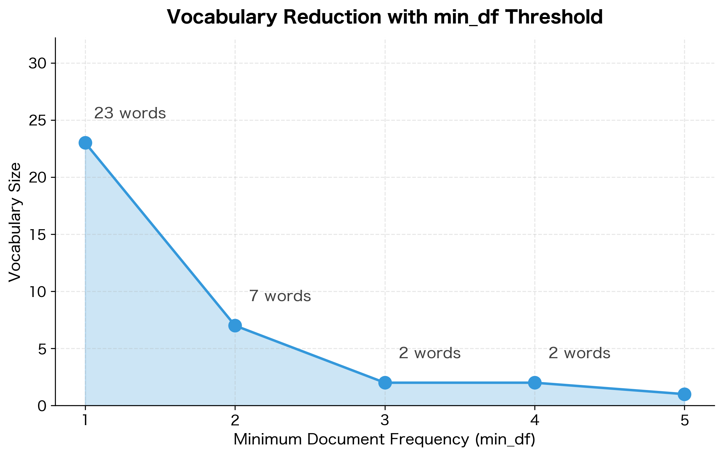
The steep drop from min_df=1 to min_df=2 is typical. In real corpora, a large fraction of words appear only once (called hapax legomena). Removing these rare words often improves model performance by reducing noise without losing much signal.
Count vs. Binary Representations
So far, we've counted word occurrences. But sometimes presence matters more than frequency. In a binary representation, each cell contains 1 if the word appears in the document and 0 otherwise, regardless of how many times it appears.
Notice that "learning" appears twice in this document. The count representation records 2, while the binary representation records 1. Which is better? It depends on the task. For document classification, binary representations often work as well as counts. For tasks where word frequency carries meaning (like authorship attribution), counts are more informative.
Sparse Matrix Representation
Real-world vocabularies contain tens of thousands of words, yet most documents use only a small fraction. A news article with 500 words might touch only 200 unique vocabulary terms out of 50,000. Storing all those zeros wastes memory.
A sparse matrix is a matrix where most elements are zero. Sparse matrix formats store only the non-zero values and their positions, dramatically reducing memory usage for high-dimensional, mostly-empty data like document-term matrices.
The Sparsity Problem
Sparsity measures the proportion of zero elements in a matrix. For a document-term matrix with documents (rows) and vocabulary words (columns), sparsity is defined as:
where:
- : the number of documents (rows in the matrix)
- : the vocabulary size (columns in the matrix)
- : the number of non-zero elements in the matrix
A sparsity of 0.99 means 99% of the matrix elements are zeros. In NLP, high sparsity is the norm because each document uses only a tiny fraction of the total vocabulary.
Let's quantify the sparsity in a typical document-term matrix:
Even in this small example, most of the matrix consists of zeros—each document only uses a fraction of the vocabulary. In real applications with vocabularies of 100,000+ words and millions of documents, sparsity typically exceeds 99%. Storing a dense matrix would require terabytes of memory for mostly zeros.
CSR Format
The Compressed Sparse Row (CSR) format stores only non-zero values along with their column indices and row boundaries. This is the standard format for document-term matrices because NLP operations typically process one document (row) at a time.
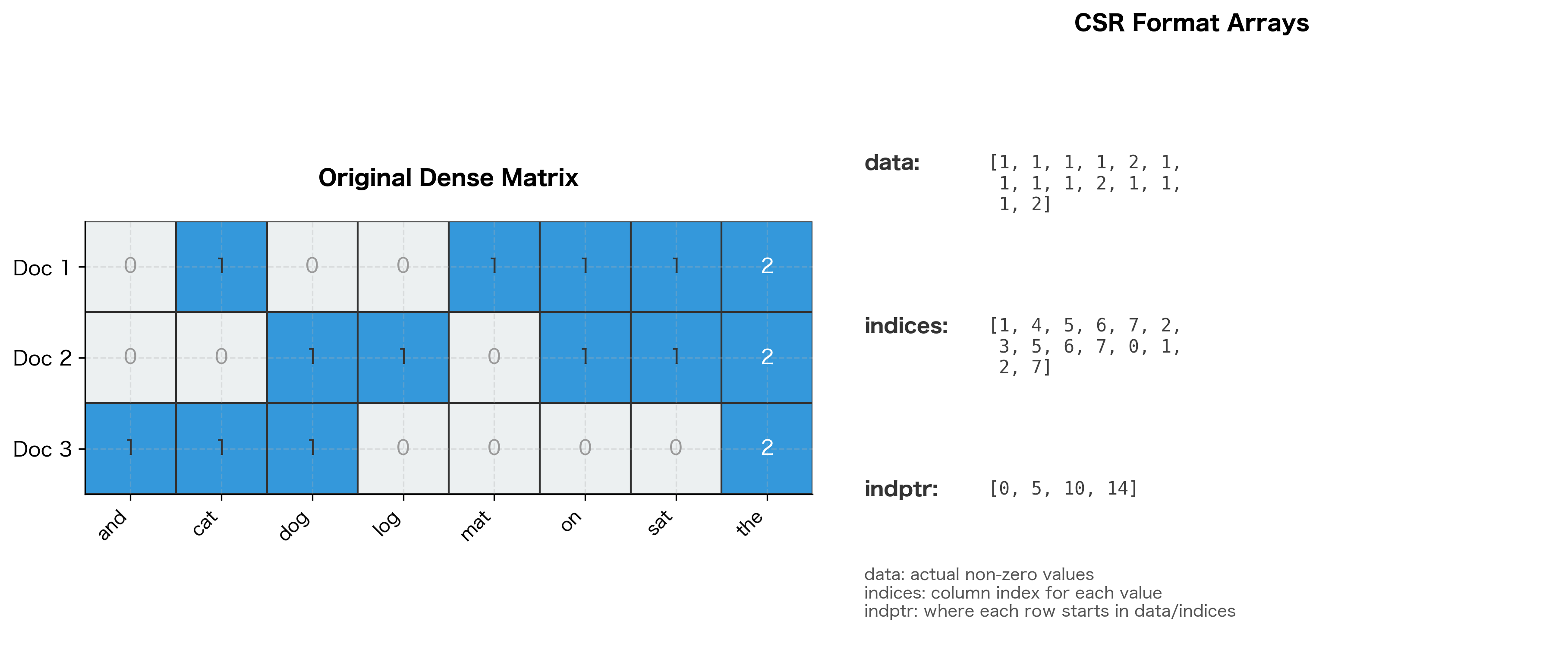
The indptr array is the key to CSR. To find the non-zero values in row , look at positions indptr[i] through indptr[i+1] in both data and indices. This makes row slicing extremely efficient.
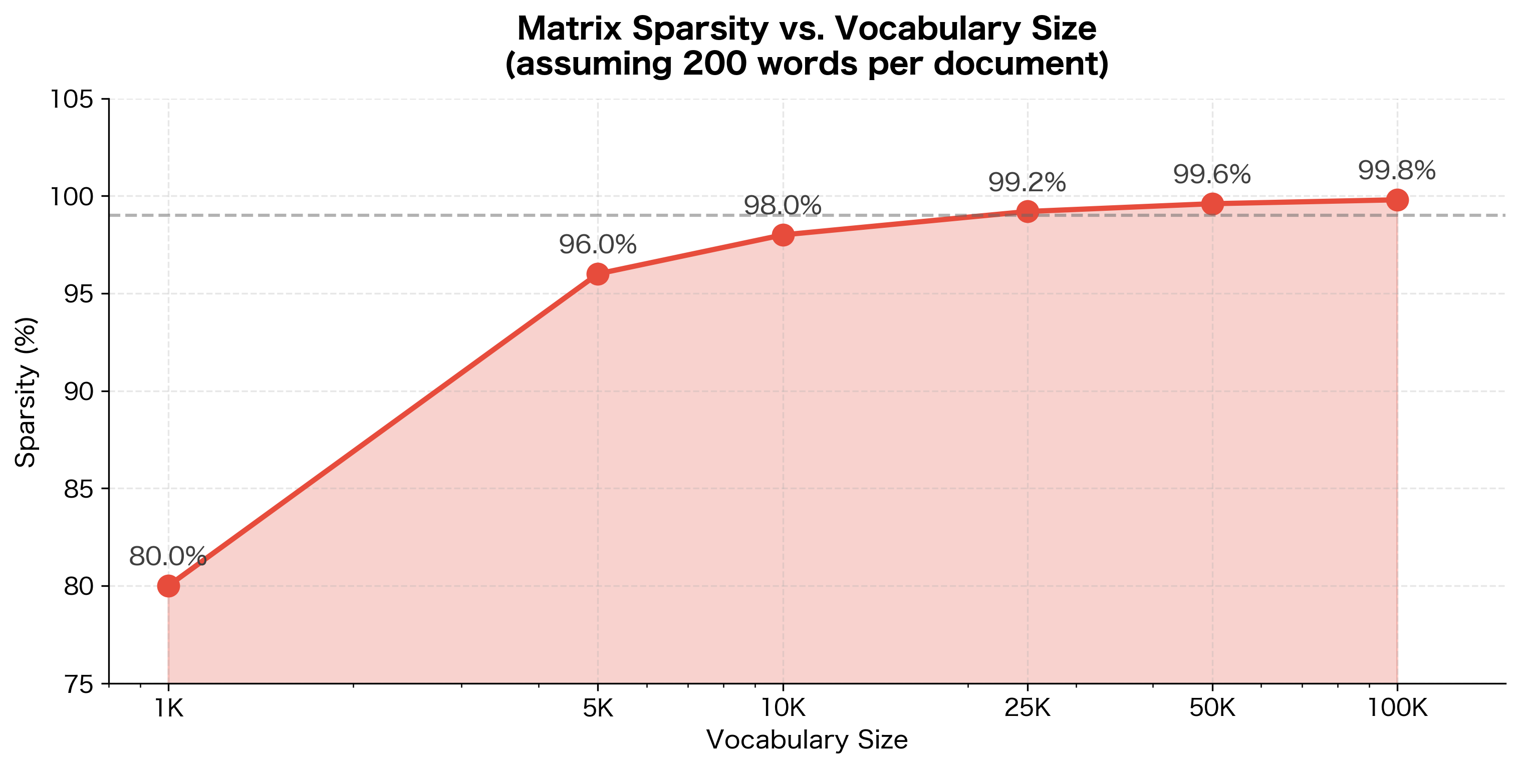
Memory Savings
The memory advantage of sparse matrices grows dramatically with vocabulary size:
For a realistic corpus of 1 million documents with a 100,000-word vocabulary, sparse representation uses less than 1% of the memory required by dense storage. This is the difference between fitting in RAM and requiring distributed storage.
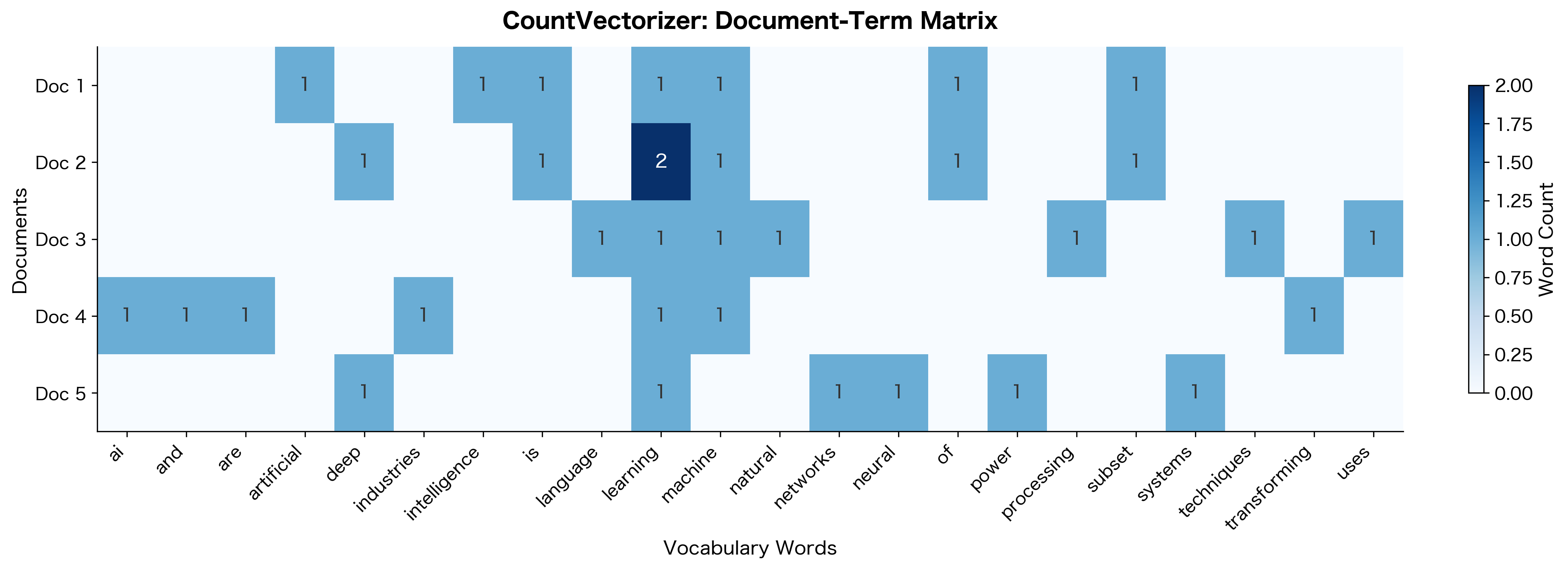
Using scikit-learn's CountVectorizer
While understanding the internals is valuable, in practice you'll use scikit-learn's CountVectorizer. It handles tokenization, vocabulary building, and sparse matrix creation in a single, optimized package.
CountVectorizer automatically handles tokenization, lowercasing, and vocabulary construction. The result is a sparse CSR matrix ready for machine learning—no manual preprocessing required.
Key Parameters
CountVectorizer offers extensive customization:
Each parameter setting produces different results. The binary setting keeps the same vocabulary but changes counts to presence indicators. Setting min_df=2 dramatically reduces vocabulary by removing rare words. The ngram_range=(1, 2) setting includes both unigrams and bigrams, capturing two-word phrases like "machine learning" and "deep learning". This dramatically increases vocabulary size but can capture meaningful phrases.
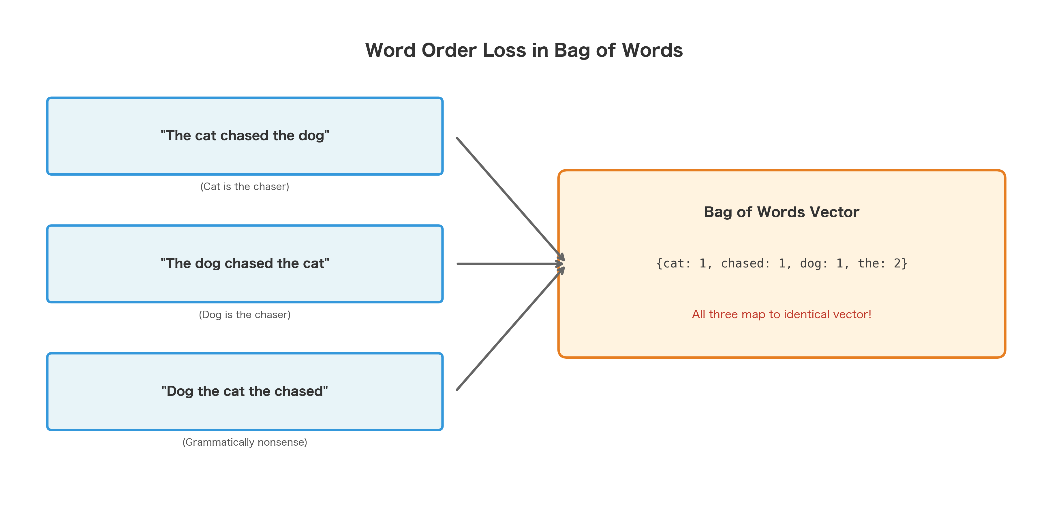
The Loss of Word Order
Bag of Words discards all structural information. "The cat chased the dog" and "The dog chased the cat" produce identical vectors, despite having opposite meanings.
This is the fundamental limitation of Bag of Words. It cannot distinguish between:
- Active and passive voice: "John hit Mary" vs "Mary was hit by John"
- Negation scope: "I love this movie" vs "I don't love this movie" have nearly identical vectors
- Questions and statements: "Is this good?" vs "This is good"
- Any semantic difference that depends on word order
When Bag of Words Works
Despite its limitations, Bag of Words remains useful for many tasks:
- Document classification: For categorizing news articles, spam detection, or sentiment analysis on long texts, word presence often matters more than order. A movie review containing "terrible", "boring", and "waste" is likely negative regardless of how those words are arranged.
- Information retrieval: Search engines match query terms against document terms. The classic TF-IDF weighting (covered in later chapters) builds directly on the Bag of Words foundation.
- Topic modeling: Algorithms like Latent Dirichlet Allocation (LDA) assume documents are mixtures of topics, each characterized by word distributions. The bag-of-words assumption is baked into the model.
- Baseline models: Before deploying complex neural networks, a BoW model provides a sanity check. If a simple model achieves 90% accuracy, you know the task is learnable from word frequencies alone.
Even this trivial example shows BoW capturing sentiment through word presence. Words like "brilliant", "fantastic", and "terrible" carry strong sentiment signals regardless of context.
Limitations and Impact
Bag of Words has fundamental limitations that motivated the development of more sophisticated representations:
- No word order: As demonstrated, BoW cannot distinguish sentences with different word arrangements.
- No semantics: "Good" and "excellent" are treated as completely unrelated words, even though they're synonyms. Similarly, "bank" (financial institution) and "bank" (river edge) are conflated.
- Vocabulary explosion: Adding n-grams helps capture some phrases but causes vocabulary size to explode. Bigrams alone can multiply vocabulary by 10-100x.
- Sparsity: High-dimensional sparse vectors are inefficient for neural networks, which prefer dense, lower-dimensional inputs.
- Out-of-vocabulary words: Words not seen during training have no representation. A model trained on formal text may fail on social media slang.
These limitations drove the development of word embeddings (Word2Vec, GloVe) and eventually transformer-based models that learn dense, contextual representations. Yet Bag of Words remains the conceptual starting point. Understanding document-term matrices, vocabulary construction, and sparse representations provides the foundation for understanding more advanced techniques.
Key Functions and Parameters
When working with Bag of Words representations, CountVectorizer from scikit-learn is the primary tool. Here are its most important parameters:
CountVectorizer(lowercase, min_df, max_df, binary, ngram_range, stop_words, max_features)
lowercase(default:True): Convert all text to lowercase before tokenizing. Set toFalseif case carries meaning (e.g., proper nouns, acronyms).min_df: Minimum document frequency threshold. If an integer, the word must appear in at least this many documents. If a float between 0.0 and 1.0, represents a proportion of documents. Usemin_df=2or higher to remove rare words and typos.max_df: Maximum document frequency threshold. Words appearing in more than this fraction of documents are excluded. Usemax_df=0.9to remove extremely common words that provide no discriminative power.binary(default:False): IfTrue, all non-zero counts are set to 1. Use binary representation when word presence matters more than frequency.ngram_range(default:(1, 1)): Tuple specifying the range of n-gram sizes to include.(1, 2)includes unigrams and bigrams, capturing phrases like "machine learning". Higher values dramatically increase vocabulary size.stop_words: Either'english'for built-in stop word list, or a custom list of words to exclude. Removes common words like "the", "is", "and" that typically add noise.max_features: Limit vocabulary to the top N most frequent terms. Useful for controlling dimensionality in very large corpora.
Summary
Bag of Words transforms text into numerical vectors by counting word occurrences, ignoring grammar and word order entirely. Despite this brutal simplification, it powers effective text classification, information retrieval, and topic modeling systems.
Key takeaways:
- Vocabulary construction extracts unique words from a corpus, mapping each to a vector dimension
- Document-term matrices represent documents as rows and vocabulary words as columns, with counts (or binary indicators) as values
- Vocabulary pruning with
min_dfandmax_dfremoves uninformative rare and common words - Sparse matrices (CSR format) efficiently store the mostly-zero document-term matrices, reducing memory by 99%+ for realistic corpora
- scikit-learn's CountVectorizer handles tokenization, vocabulary building, and sparse matrix creation in one optimized package
- Word order loss is the fundamental limitation: "The cat chased the dog" and "The dog chased the cat" produce identical vectors
In the next chapters, we'll extend these ideas with n-grams to capture some word sequences, and with TF-IDF weighting to emphasize discriminative terms over common ones.
Quiz
Ready to test your understanding? Take this quick quiz to reinforce what you've learned about Bag of Words representations.

Comments