N-gram Language Models: Probability and Text Generation

What makes some word sequences sound natural while others feel wrong? "The cat sat on the mat" flows effortlessly, but "mat the on sat cat the" is gibberish even though it contains exactly the same words. Native speakers intuitively know which sequences are probable, even for sentences they have never heard before. N-gram language models capture this intuition mathematically, assigning probabilities to sequences of words based on patterns learned from large text collections.

Language models are foundational to natural language processing. They power spell checkers that suggest "their" over "thier," autocomplete systems that predict your next word, and speech recognizers that disambiguate "recognize speech" from "wreck a nice beach." Before neural networks dominated the field, n-gram models were the workhorses of language modeling. Systems built on trigrams and simple smoothing techniques ran at the heart of Google's search products, Microsoft's Bing, and virtually every production voice interface from the 1990s through the early 2010s. Understanding them provides essential intuition for the modern approaches covered throughout this handbook.

As we saw in the previous chapter on N-grams, sequences of adjacent words reveal statistical patterns in text. This chapter takes that idea further: instead of simply counting n-gram frequencies, we use those counts to build a probability model over entire word sequences. You will learn the probability theory that makes n-gram language models work, implement them from scratch, evaluate them rigorously with perplexity, and discover both their power and their fundamental limitations. The next chapter on Smoothing Techniques addresses the central failure mode you will encounter here.

A language model assigns probabilities to sequences of words. Given a sequence of $n$ words, denoted $w_1, w_2, \ldots, w_n$, the model estimates $P(w_1, w_2, \ldots, w_n)$, the probability of that exact sequence occurring in natural language. Here $w_i$ represents the $i$-th word in the sequence. For example, $w_1$ might be "the" and $w_2$ might be "cat."

Why is assigning probabilities to word sequences useful? The applications are remarkably broad.

Disambiguation. A speech recognition system hears an ambiguous audio signal. It might produce two candidate transcriptions: "I saw a van" and "eyes awe of an." A language model knows the first sequence is far more probable and helps the system choose correctly. The acoustic model tells you what sounds were produced; the language model tells you which word sequence those sounds most plausibly correspond to.

Ranking. A machine translation system generates dozens of candidate translations for a source sentence. A language model scores each candidate by how natural it sounds in the target language, allowing the system to prefer fluent output over grammatically awkward but technically accurate alternatives.

Generation. If we can compute $P(w_1, \ldots, w_n)$ for any sequence, we can generate new text by sampling words according to their probabilities given the preceding context. Start from the beginning of a sentence, pick the next word proportionally to its probability, advance the window, and repeat. This same generation mechanism, refined and scaled enormously, underlies modern large language models like GPT-4.

Evaluation. A language model provides a principled way to measure how "natural" a corpus is. Lower perplexity under the model means the text fits the learned distribution more closely, which makes language models useful for detecting out-of-domain text, machine-generated content, or low-quality data.

Computing the probability of a full sequence seems daunting at first. How could we possibly estimate $P(\text{"the cat sat on the mat"})$ directly? We would need to count how often this exact six-word sequence appears in training data, then divide by the total number of six-word sequences. But most sentences are unique. Even in a corpus of billions of words, we are unlikely to see any specific sentence more than a handful of times. For longer sentences, the chance of observing a particular sequence approaches zero.

The chain rule of probability offers an escape from this dilemma. Instead of estimating the joint probability directly, we decompose it into a product of conditional probabilities. Each conditional probability asks a simpler question: given everything that came before, how likely is the next word?

The chain rule derives from the definition of conditional probability. Conditional probability is defined as:

$$P(A|B) = \frac{P(A, B)}{P(B)}$$

where:

• $P(A|B)$: the probability of event $A$ occurring given that event $B$ has already occurred
• $P(A, B)$: the joint probability of both $A$ and $B$ occurring together
• $P(B)$: the probability of event $B$ occurring, serving as the normalizing denominator

Rearranging gives the multiplication rule: $P(A, B) = P(B) \times P(A|B)$. The probability of both events equals the probability of the first event times the probability of the second event given the first. For a sequence of words, we apply this rule repeatedly to break down the joint probability into simpler conditional probabilities.

Step 1: Start with the joint probability of all words:

$$P(w_1, w_2, \ldots, w_n)$$

Step 2: Apply the multiplication rule to separate the last word, treating "all words up to $w_{n-1}$" as event $B$ and "$w_n$ appears next" as event $A$:

$$P(w_1, \ldots, w_n) = P(w_1, \ldots, w_{n-1}) \times P(w_n|w_1, \ldots, w_{n-1})$$

Step 3: Apply the same rule recursively to $P(w_1, \ldots, w_{n-1})$, peeling off one word at a time, until only $P(w_1)$ remains:

$$\begin{aligned} P(w_1, w_2, \ldots, w_n) &= P(w_1) \times P(w_2|w_1) \times P(w_3|w_1, w_2) \times \cdots \times P(w_n|w_1, \ldots, w_{n-1}) \end{aligned}$$

Using product notation, this is written compactly as:

$$P(w_1, \ldots, w_n) = \prod_{i=1}^{n} P(w_i|w_1, \ldots, w_{i-1})$$

where:

• $w_i$: the $i$-th word in the sequence
• $P(w_i|w_1, \ldots, w_{i-1})$: the conditional probability of word $w_i$ given all preceding words, the "history"
• $\prod_{i=1}^{n}$: the product operator, which multiplies all $n$ terms together

The probability of a sequence equals the probability of the first word, times the probability of the second word given the first, times the probability of the third word given the first two, and so on. Each step conditions on all previously observed words.

This decomposition is mathematically exact, not an approximation. The chain rule holds for any joint distribution, regardless of how complex the dependencies between words are.

Let us see this decomposition in action with a concrete example:

Each term in this product answers a progressively more specific question. The first asks: how likely is "the" to start a sentence? The second asks: given we started with "the," how likely is "cat" to follow? By the time we reach the final word, we are asking: given the entire context "the cat sat on the," how likely is "mat"?

The chain rule is mathematically exact, but it creates a severe practical problem. To compute $P(w_n|w_1, \ldots, w_{n-1})$, we need the probability of word $w_n$ given the entire preceding context. For long sentences, this context can be arbitrarily long. A 20-word sentence requires estimating the probability of the 20th word given all 19 preceding words. We will never have enough training data to estimate these long-context probabilities reliably, since most 19-word contexts appear only once, if ever. The number of distinct 19-word contexts in any finite corpus is essentially as large as the corpus itself.

This is where the Markov assumption comes in.

The chain rule gives us an exact decomposition, but it demands something impractical: reliable estimates of probabilities conditioned on arbitrarily long histories. The key insight of n-gram models is to make a simplifying assumption that trades some accuracy for tractability.

The assumption is named after the Russian mathematician Andrey Markov, who studied stochastic processes with this "memoryless" property in the early 20th century. In a Markov chain, the probability of the next state depends only on the current state, not on the full history of how you arrived there. In the context of language, it means we assume the future depends only on the recent past, not the distant past.

For a unigram model ($n = 1$), each word is treated as completely independent of all others:

$$P(w_i|w_1, \ldots, w_{i-1}) \approx P(w_i)$$

The unigram model ignores all context. It assigns the same probability to "cat" whether the preceding words were "the fluffy" or "the entire concept of." This is obviously a poor approximation, but unigrams are useful as a baseline and as a component in more sophisticated models.

For a bigram model ($n = 2$), each word depends only on the single word immediately before it:

$$P(w_i|w_1, \ldots, w_{i-1}) \approx P(w_i|w_{i-1})$$

where:

• $P(w_i|w_1, \ldots, w_{i-1})$: the true conditional probability given the full history (left side)
• $P(w_i|w_{i-1})$: the bigram approximation using only the immediately preceding word (right side)
• $\approx$: indicates this is an approximation, not an equality

For a trigram model ($n = 3$), the memory extends to two previous words:

$$P(w_i|w_1, \ldots, w_{i-1}) \approx P(w_i|w_{i-2}, w_{i-1})$$

where:

• $w_{i-2}$: the word two positions before the current word
• $w_{i-1}$: the word immediately before the current word
• The context $(w_{i-2}, w_{i-1})$ forms a two-word history window

In general, for an n-gram model, the Markov approximation is:

$$P(w_i|w_1, \ldots, w_{i-1}) \approx P(w_i|w_{i-n+1}, \ldots, w_{i-1})$$

where the context window spans exactly $n-1$ preceding words. We discard information from the distant past to make estimation tractable from finite data.

Why does this help? Consider the difference in what we need to estimate for the sentence "the cat sat on the mat":

• Full history: We need $P(\text{mat}|\text{the cat sat on the})$, requiring counts of the specific five-word context.
• Trigram: We need $P(\text{mat}|\text{on the})$, requiring only counts of the two-word context.
• Bigram: We need $P(\text{mat}|\text{the})$, requiring only counts of the single word "the."

Shorter contexts appear far more frequently in training data, giving us more reliable probability estimates. The Markov assumption is an approximation, but it works surprisingly well in practice because language has enough local structure that nearby words carry most of the predictive information. The word that most immediately constrains "mat" is likely "the" (or "on the"), not the first word five positions back.

With the Markov assumption in hand, we have reduced our problem to estimating conditional probabilities like $P(\text{mat}|\text{on the})$. But how do we compute these from data?

The most straightforward approach is maximum likelihood estimation (MLE): count how often each n-gram appears in our training corpus, then normalize. For a given context, the MLE probability of the next word is simply the fraction of times that word followed that context in training.

The MLE formula follows directly from the definition of conditional probability. Recall that conditional probability is defined as the joint probability of both events divided by the marginal probability of the conditioning event:

$$P(B|A) = \frac{P(A, B)}{P(A)}$$

To estimate $P(w_i|w_{i-1})$ from training data, we approximate each probability with its empirical relative frequency. The joint probability $P(w_{i-1}, w_i)$ is approximated by how often the pair $(w_{i-1}, w_i)$ occurs, divided by the total number of bigrams. The marginal probability $P(w_{i-1})$ is approximated by how often $w_{i-1}$ occurs, divided by the total number of words.

When we compute the ratio, the denominators cancel, and we are left with:

$$P(w_i|w_{i-1}) = \frac{C(w_{i-1}, w_i)}{C(w_{i-1})}$$

where:

• $C(w_{i-1}, w_i)$: the count of times the bigram $(w_{i-1}, w_i)$ appears consecutively in the training corpus
• $C(w_{i-1})$: the count of times the context word $w_{i-1}$ appears anywhere in the corpus
• The ratio gives the proportion of $w_{i-1}$ occurrences that are followed by $w_i$

Worked example: If "the" appears 100 times in our corpus and "the cat" appears 8 times, then:

$$P(\text{cat}|\text{the}) = \frac{C(\text{the, cat})}{C(\text{the})} = \frac{8}{100} = 0.08$$

This means 8% of the time "the" is followed by "cat."

For trigrams, we extend the same logic to two-word contexts:

$$P(w_i|w_{i-2}, w_{i-1}) = \frac{C(w_{i-2}, w_{i-1}, w_i)}{C(w_{i-2}, w_{i-1})}$$

where:

• $C(w_{i-2}, w_{i-1}, w_i)$: the count of the trigram (three consecutive words)
• $C(w_{i-2}, w_{i-1})$: the count of the two-word context alone (the bigram prefix)

The general MLE formula for any n-gram order is:

$$P(w_i|w_{i-n+1}, \ldots, w_{i-1}) = \frac{C(w_{i-n+1}, \ldots, w_{i-1}, w_i)}{C(w_{i-n+1}, \ldots, w_{i-1})}$$

where:

• $w_i$: the word whose probability we want to estimate
• $w_{i-n+1}, \ldots, w_{i-1}$: the context of $n-1$ words immediately preceding $w_i$
• $C(w_{i-n+1}, \ldots, w_{i-1}, w_i)$: the count of the complete n-gram in the training corpus
• $C(w_{i-n+1}, \ldots, w_{i-1})$: the count of the $(n-1)$-gram context alone

The formula always divides the count of the full n-gram by the count of its $(n-1)$-gram prefix. This relative frequency estimate is the maximum likelihood solution because it maximizes the probability of observing the training data under the model. No other choice of conditional probability parameters would assign a higher likelihood to the observed training corpus. If you were to increase any single $P(w|context)$ above the relative frequency estimate, you would have to decrease the probability of other words following that context, and the net effect would be a decrease in training data likelihood.

Let us implement this and see it work on a small corpus:

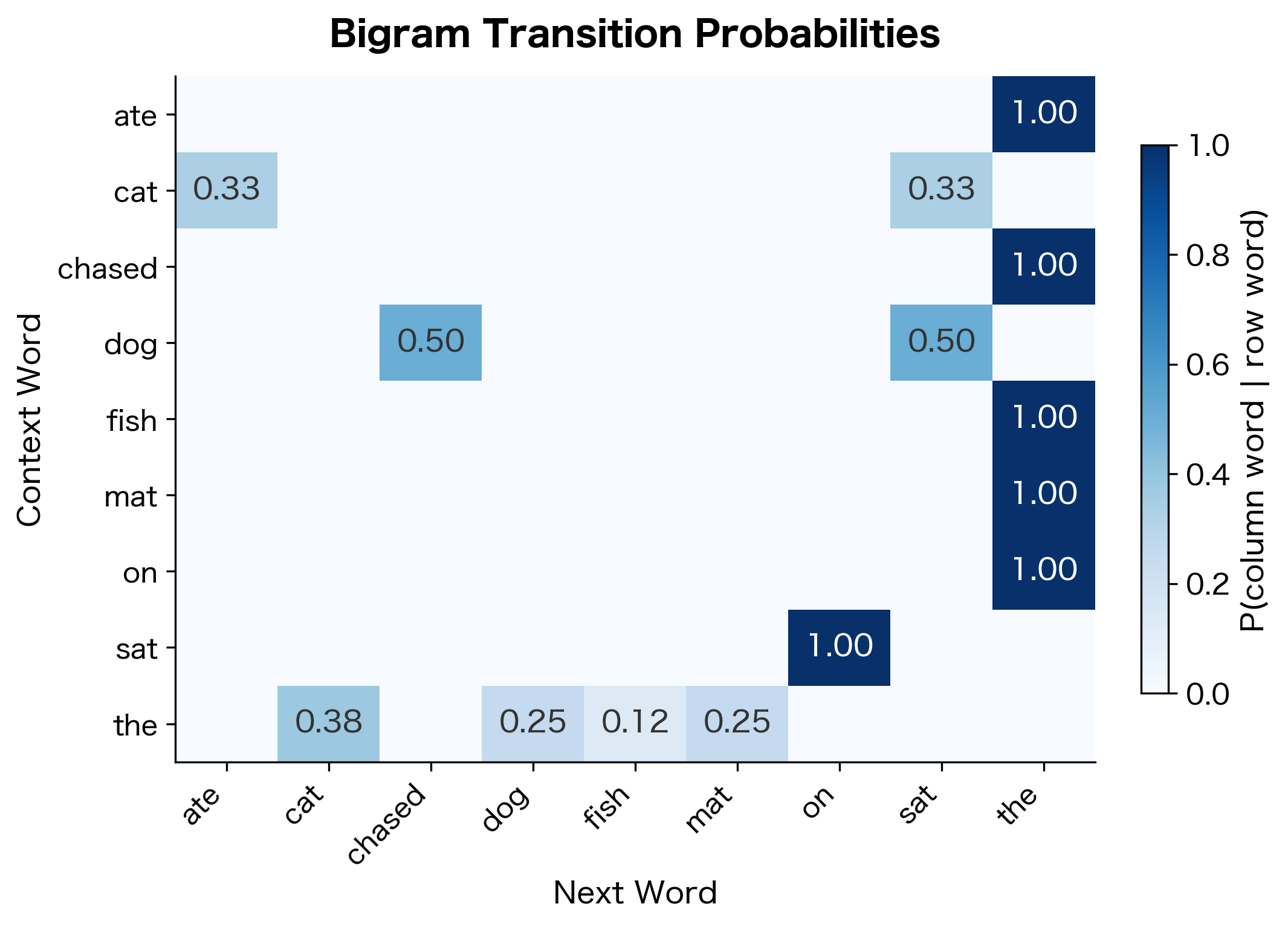
The heatmap reveals the sparse structure of bigram probabilities. Most cells are empty (zero probability), indicating word pairs that never occurred in our corpus. The non-zero cells cluster around specific patterns: "the" can be followed by several words, but "sat" is always followed by "on." This sparsity becomes even more pronounced with larger vocabularies and higher-order n-grams. With a real vocabulary of 50,000 words, the matrix would be 50,000 by 50,000 with the overwhelming majority of cells set to zero.

Sentences have beginnings and endings, and a language model needs to capture both. We add special boundary tokens: <s> marks the start of a sentence and </s> marks the end. These tokens allow the model to learn which words typically begin sentences and which words tend to end them.

Without boundary tokens, a bigram model cannot distinguish words that begin sentences from words that appear mid-sentence. If "the" starts every sentence in our corpus, the model should assign high probability to "the" appearing after the sentence boundary. But without a boundary token, there is no special context to condition on for sentence-initial words. The start token <s> provides a synthetic context that captures sentence-initial patterns, enabling the model to compute $P(w_1|\text{<s>})$, the probability of a word starting a sentence.

The end token </s> is equally important. Without it, the model has no mechanism to learn when sentences typically end. A generation system using the model would need an external stopping criterion. With </s> in the vocabulary, the model learns to assign probability to sentence endings, and generation naturally terminates when </s> is sampled.

The start marker <s> lets us compute $P(w_1|\text{<s>})$, the probability of a word starting a sentence. In our corpus, "the" starts every sentence, so $P(\text{the}|\text{<s>}) = 1.0$. The end marker </s> lets us model sentence endings: "mat," "fish," and "cat" all end sentences.

For higher-order n-grams, we add multiple start tokens. A trigram model needs two <s> tokens at the beginning to provide context for the first two content words. A 4-gram model needs three start tokens. The general rule: prepend $n-1$ start tokens for an order-$n$ model. This ensures that even the very first content words in a sentence have a full context of length $n-1$ available.

With n-gram probabilities estimated, we can compute the probability of any sequence. We combine the chain rule decomposition with the Markov approximation to get:

$$P(w_1, \ldots, w_m) \approx \prod_{i=1}^{m} P(w_i|w_{i-n+1}, \ldots, w_{i-1})$$

where:

• $m$: the total number of words in the sequence
• $n$: the n-gram order (2 for bigrams, 3 for trigrams)
• $w_i$: the $i$-th word in the sequence
• $w_{i-n+1}, \ldots, w_{i-1}$: the context of $n-1$ words immediately preceding $w_i$
• $\prod_{i=1}^{m}$: multiply all $m$ conditional probabilities together

For a bigram model ($n = 2$), this simplifies to:

$$P(w_1, \ldots, w_m) \approx P(w_1|\text{<s>}) \times P(w_2|w_1) \times P(w_3|w_2) \times \cdots \times P(w_m|w_{m-1})$$

where:

• $P(w_1|\text{<s>})$: the probability of the first word given the start-of-sentence marker
• $P(w_i|w_{i-1})$: the probability of each subsequent word given only the single preceding word

Multiplying many small probabilities leads to numerical underflow: numbers become too small to represent in floating-point arithmetic. A sentence of 300 words, each with probability 0.1, gives $0.1^{300} = 10^{-300}$, close to the minimum representable double-precision float near $5 \times 10^{-324}$. Longer sentences or lower-probability words make this worse. Taking logarithms converts products to sums, keeping values in a manageable range.

Instead of computing a product of probabilities:

$$P(w_1, \ldots, w_m) = \prod_{i=1}^{m} P(w_i|w_{i-1})$$

we compute a sum of log probabilities:

$$\log P(w_1, \ldots, w_m) = \sum_{i=1}^{m} \log P(w_i|w_{i-1})$$

where:

• $\log$: the natural logarithm function (base $e \approx 2.718$)
• $\sum_{i=1}^{m}$: sum over all $m$ words in the sequence
• $\log P(w_i|w_{i-1})$: the log probability of each bigram conditional, always a negative number since $0 < P < 1$

This transformation works because of the logarithm's fundamental property: $\log(a \times b) = \log(a) + \log(b)$. While individual probabilities might be 0.01 or smaller, their log values are manageable negative numbers (for example, $\log(0.01) \approx -4.6$). To recover the original probability if needed, compute $P = \exp(\log P)$.

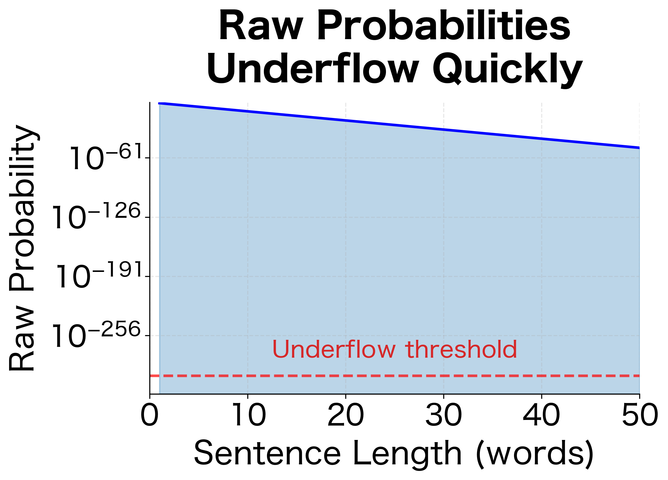
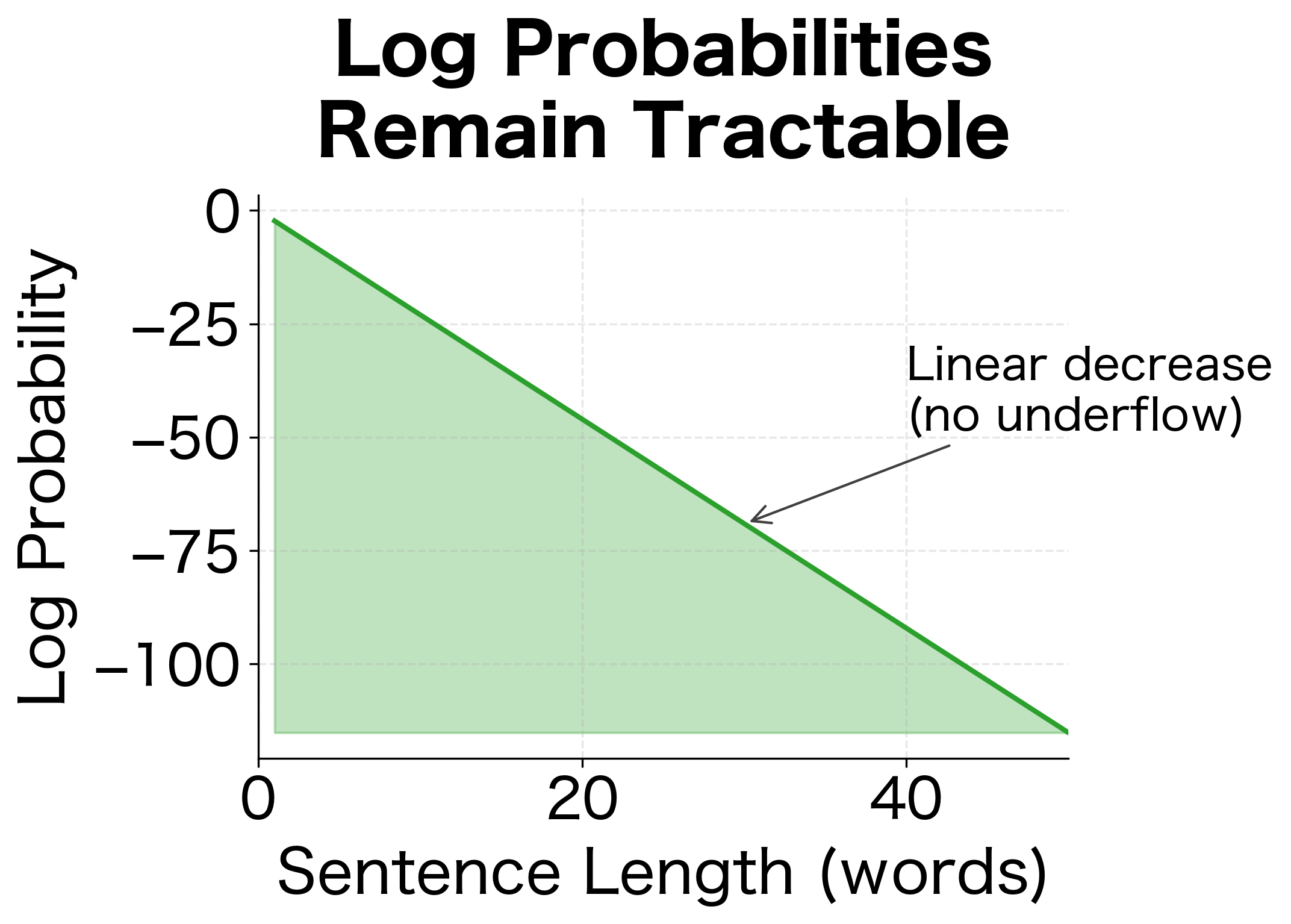
The visualization confirms why log probabilities are essential. With an average per-word probability of 0.1, raw probabilities approach the limits of floating-point representation at around 300 words. Log probabilities decrease linearly and remain tractable for sequences of any length.

What happens when we encounter an n-gram that never appeared in training?

A single unseen bigram makes the entire sequence probability zero. This is the zero probability problem: perfectly valid sentences receive zero probability just because our training data did not contain every possible word combination. The sentence "the bird flew over the house" is entirely plausible English, but our tiny corpus knows nothing about birds or flying. The MLE estimate assigns probability zero to any n-gram not seen in training, and since sequence probability is a product of these terms, any zero drives the whole product to zero.

The deeper issue is that zero probability is semantically wrong, in addition to being numerically inconvenient. A language model that assigns zero probability to valid English sentences fundamentally misrepresents the distribution of language. A well-calibrated language model should assign some small but non-zero probability to any grammatical sequence. This brittleness motivates smoothing techniques, covered in the next chapter. Raw MLE estimates are too brittle for real applications since any test sentence containing an unseen n-gram collapses to zero probability regardless of its plausibility.

So far we have talked about probability as the goal of language modeling, but how do we measure whether one language model is better than another? We need an evaluation metric that captures how well a model assigns probability to new, held-out text.

The most widely used evaluation metric for language models is perplexity. Perplexity measures how "surprised" a model is by new text. A model that assigns high probability to the test data is not very surprised, giving low perplexity. A model that assigns low probability to the test data is very surprised, giving high perplexity.

Perplexity is defined as the inverse probability of the test set, normalized by the number of words. For a test sequence $W = w_1, w_2, \ldots, w_N$ of $N$ words, perplexity is:

$$\text{PP}(W) = P(w_1, w_2, \ldots, w_N)^{-1/N}$$

where:

• $P(w_1, w_2, \ldots, w_N)$: the probability assigned to the test sequence by the model
• $-1/N$: the exponent normalizes for sequence length, so longer sequences are comparable to shorter ones
• The outer operation takes the $N$-th root (or equivalently, raises to the power $-1/N$)

Expanding the sequence probability using the chain rule, perplexity becomes:

$$\text{PP}(W) = \left(\prod_{i=1}^{N} P(w_i|w_1, \ldots, w_{i-1})\right)^{-1/N}$$

Using the n-gram Markov approximation for a bigram model:

$$\text{PP}(W) = \left(\prod_{i=1}^{N} P(w_i|w_{i-1})\right)^{-1/N}$$

This is equivalent to the geometric mean of the inverse bigram probabilities. Minimizing perplexity is equivalent to maximizing the log probability of the test set per word.

In practice, we compute perplexity in log space to avoid numerical underflow:

$$\begin{aligned} \log \text{PP}(W) &= -\frac{1}{N} \log P(W) \\ &= -\frac{1}{N} \sum_{i=1}^{N} \log P(w_i|w_{i-1}) \end{aligned}$$

and then exponentiate:

$$\text{PP}(W) = \exp\!\left(-\frac{1}{N} \sum_{i=1}^{N} \log P(w_i|w_{i-1})\right)$$

where:

• $N$: number of words in the test set
• $\log P(w_i|w_{i-1})$: log probability of each word given its context (a negative number)
• The average negative log probability gives the per-word entropy in nats
• Exponentiating converts entropy back to a perplexity value

Perplexity has an intuitive interpretation as the effective branching factor of the language model. If every word has exactly the same number of equally likely continuations, perplexity equals that branching factor. A perplexity of 100 means the model is as confused as if it were choosing uniformly among 100 equally likely options at each step.

Consider the extremes:

• Perplexity = 1: The model is perfectly certain about every word. Given the context, only one continuation is possible. This happens when text is entirely predictable (like a model evaluated on its own training data with no unseen n-grams).
• Perplexity = V (vocabulary size): The model is completely uncertain, equivalent to a uniform distribution over all vocabulary words. This happens when context provides no information.
• Perplexity in between: Real language models fall somewhere between these extremes. A good bigram model on English text might achieve a perplexity of 50 to 200, depending on the corpus and vocabulary.

Lower perplexity is always better, but the absolute value matters less than relative comparisons between models evaluated on the same test set.

Let us build a reusable n-gram language model class that encapsulates everything we have covered so far:

The results reveal key differences between model orders. The unigram model assigns similar probabilities to all sentences because it ignores word order entirely. The bigram model shows more variation, penalizing sentences with rare or unseen word transitions. The trigram model provides the finest discrimination. On training data, perplexity decreases with increasing n-gram order because more context allows more precise predictions. On held-out data with a small training corpus, this pattern can reverse if higher-order n-grams are too sparse.

Perplexity has a deep connection to information theory. The entropy of a language model is:

$$H(W) = -\frac{1}{N} \sum_{i=1}^{N} \log_2 P(w_i|w_1, \ldots, w_{i-1})$$

where:

• $H(W)$: the per-word entropy in bits
• $N$: total number of words in the test set
• $\log_2$: logarithm base 2 converts to bits
• The entropy measures the average number of bits needed to encode each word given perfect context

Perplexity is simply $2^{H(W)}$ when using log base 2, or $\exp(H(W))$ when using natural logarithms. A perplexity of 100 corresponds to an entropy of about 6.6 bits per word, meaning the model is about as uncertain as if it had to choose uniformly among 100 equally likely options at each step.

This connection to information theory has a practical interpretation: a model with perplexity $k$ requires approximately $\log_2(k)$ bits per word to encode text under that model. Lower perplexity means more compressible text, which means the model has captured more of the statistical regularities in the language.

Choosing the right n-gram order involves a fundamental tradeoff: more context yields better predictions, but more context also means sparser counts and more zero probabilities.

A unigram model treats every word independently and assigns the same probability to "the cat" and "the mat." A bigram model knows that "cat" frequently follows "the" but "xkcd" rarely does. A trigram model additionally knows that "sat on the" is a common pattern while "flew under the" is unusual in most corpora. A 4-gram model can capture even longer dependencies, like the fact that "I would like to" commonly continues with a verb.

As n-gram order increases, the number of possible n-grams grows exponentially:

$$\text{Possible n-grams} = V^n$$

where:

• $V$: the vocabulary size (number of unique word types)
• $n$: the n-gram order
• $V^n$: exponential growth, so each additional word of context multiplies the parameter count by $V$

For English with $V = 100{,}000$ words and $n = 3$ (trigrams), we have $100{,}000^3 = 10^{15}$ potential trigrams. Even storing just one byte per trigram would require a petabyte of memory. Fortunately, the vast majority of combinations never occur in real text, so sparse storage structures (dictionaries or tries) are practical.

The deeper problem is not storage but coverage. Even with enormous corpora, higher-order n-grams remain sparse:

The coverage statistics explain why simply using more context is not an obvious win. Yes, a 5-gram model can condition on four words of context, but 85% of the time it will encounter a 5-gram it has never seen and must fall back to some default. In practice, trigram models ($n = 3$) were the standard choice for production NLP systems before neural language models, balancing context length against manageable sparsity.

The plots use our small training corpus but illustrate the key pattern: as order increases, both the count of observed n-grams grows (because there are more distinct longer sequences) and coverage of the theoretical maximum collapses (because the space grows much faster than the data).

Our toy corpus produces tiny models measured in kilobytes. Real-world models trained on billions of words require a completely different approach to storage. Production systems typically use trie-based storage, where each path from the root to a node represents an n-gram prefix and nodes store counts and probabilities. Tries share prefixes between n-grams, reducing memory and enabling efficient prefix queries. The ARPA language model format, used by tools like KenLM and SRILM, stores n-gram counts and back-off weights in a text format that most speech recognition and MT systems can read. KenLM further compresses this using sorted arrays, reducing a multi-gigabyte text file to a few hundred megabytes in binary format.

N-gram models can generate new text by sampling words according to their conditional probabilities. Starting from the start token, we repeatedly sample the next word given the current context, then advance the context window by one position.

The generation algorithm is simple: maintain a sliding window of the last $n-1$ words (the context), look up all words that have appeared after that context in training, sample from the distribution, add the sampled word to the output and to the context window, and repeat until </s> is generated or a maximum length is reached.

The bigram model generates sentences that reflect local word patterns from the training data. The trigram model maintains coherence over slightly longer distances since it sees two words of context at each step. Both models tend to produce sentences similar to those in the training corpus: this is a feature, not a bug, since the models have learned the statistical patterns of the training text. With a larger and more diverse training corpus, the generated text would reflect the full variety of patterns the model has seen.

We can control the randomness of generation with a temperature parameter $T$. Temperature scaling adjusts the probability distribution over next words before sampling, sharpening it (more deterministic) or flattening it (more exploratory).

The idea is to scale log probabilities by dividing by $T$ before re-normalizing:

$$P_T(w_i) = \frac{\exp\!\left(\log P(w_i) / T\right)}{\sum_j \exp\!\left(\log P(w_j) / T\right)}$$

where:

• $P(w_i)$: the original probability of word $w_i$ from the language model
• $T$: the temperature parameter, a positive real number typically between 0.1 and 2.0
• $\log P(w_i) / T$: dividing the log probability by $T$ amplifies or compresses differences between words
• $\exp(\cdot)$: converts the scaled log probability back to a positive number for normalization
• The denominator normalizes the result so all probabilities sum to 1

The temperature controls the shape of the distribution:

• $T < 1$ (low temperature): Differences in log probability are amplified, sharpening the distribution and concentrating probability on the most likely words.
• $T = 1$: Uses the original probabilities unchanged.
• $T > 1$ (high temperature): Differences are compressed, flattening the distribution and giving rare words more chance.

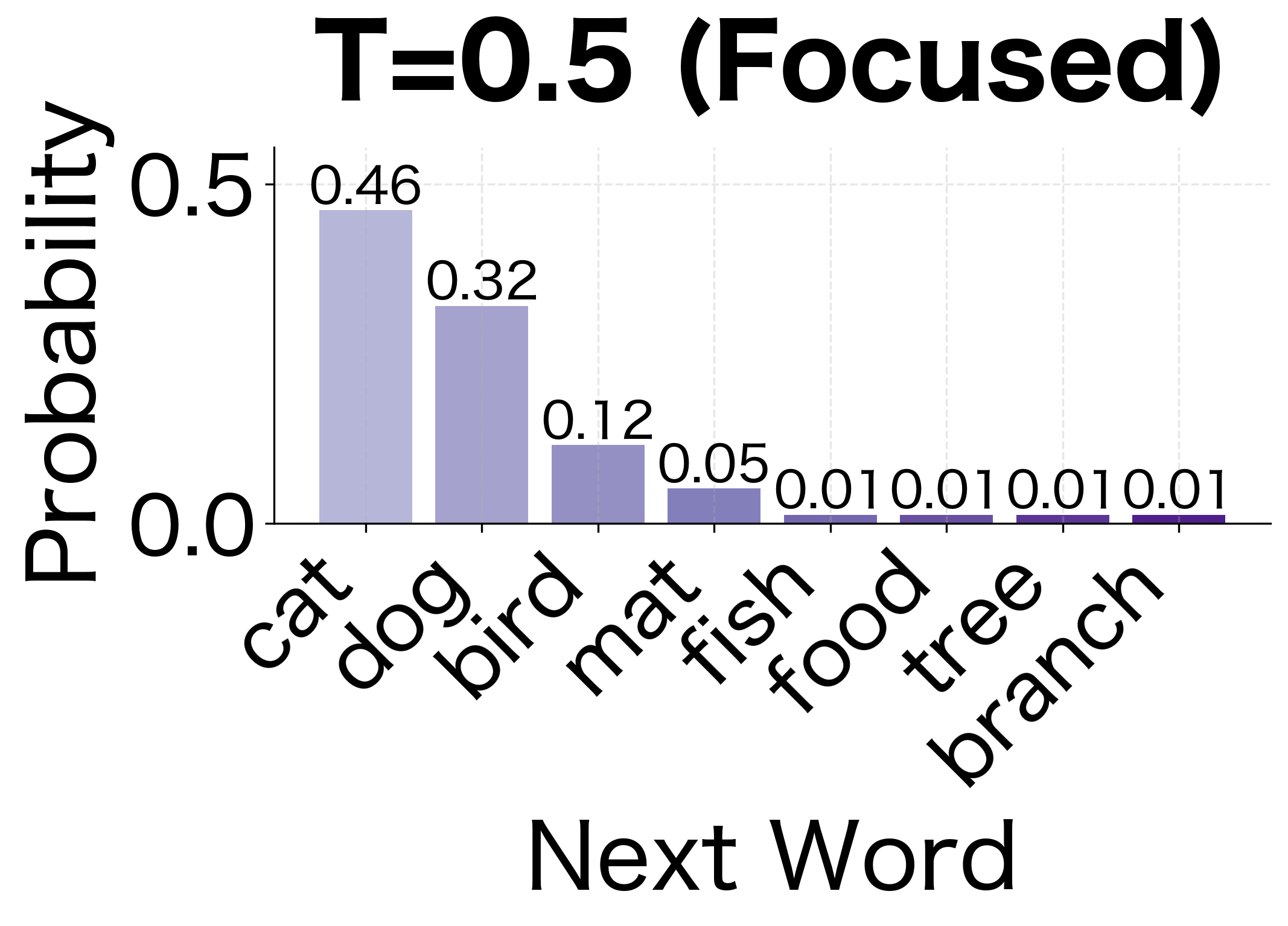
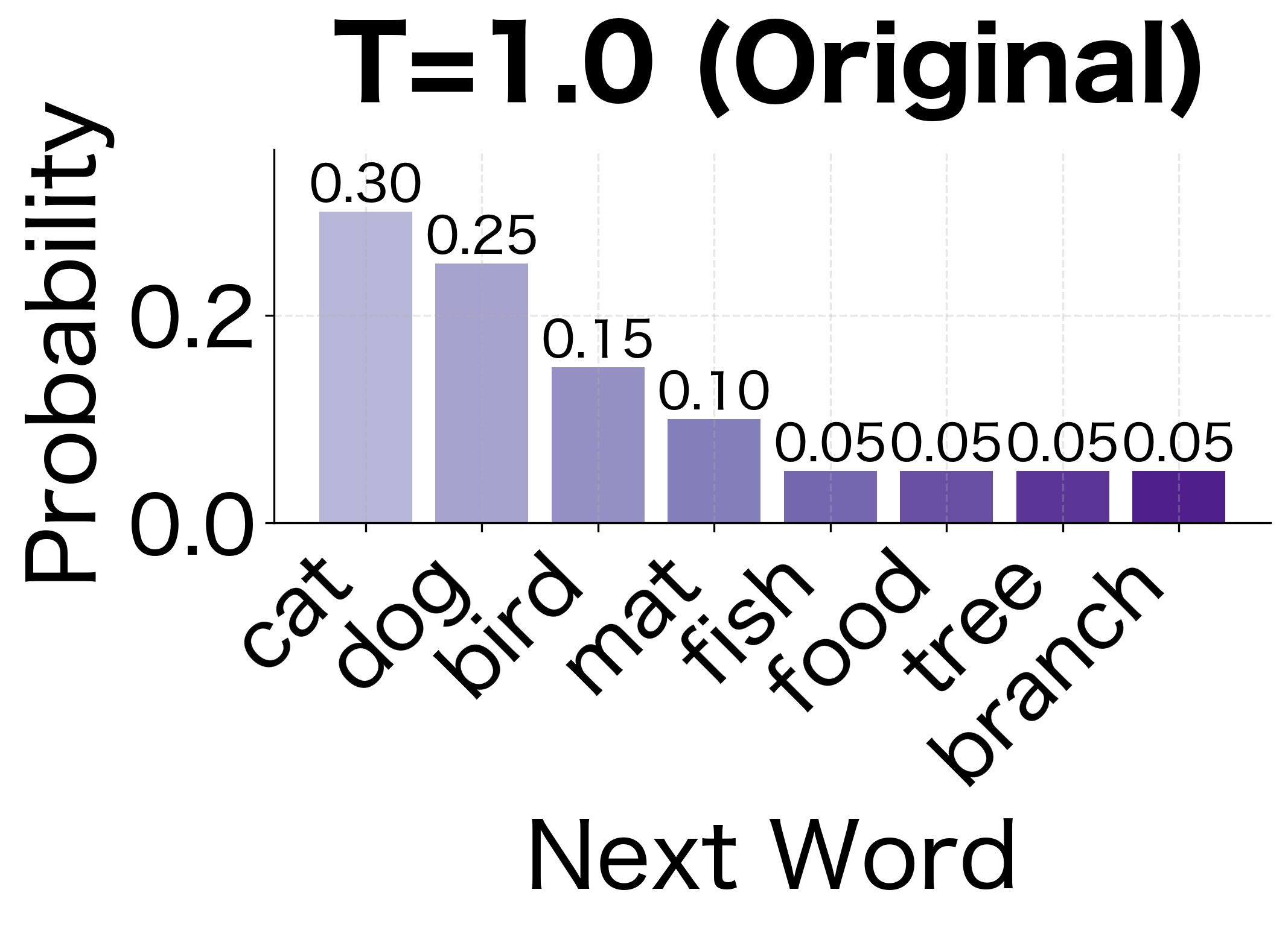
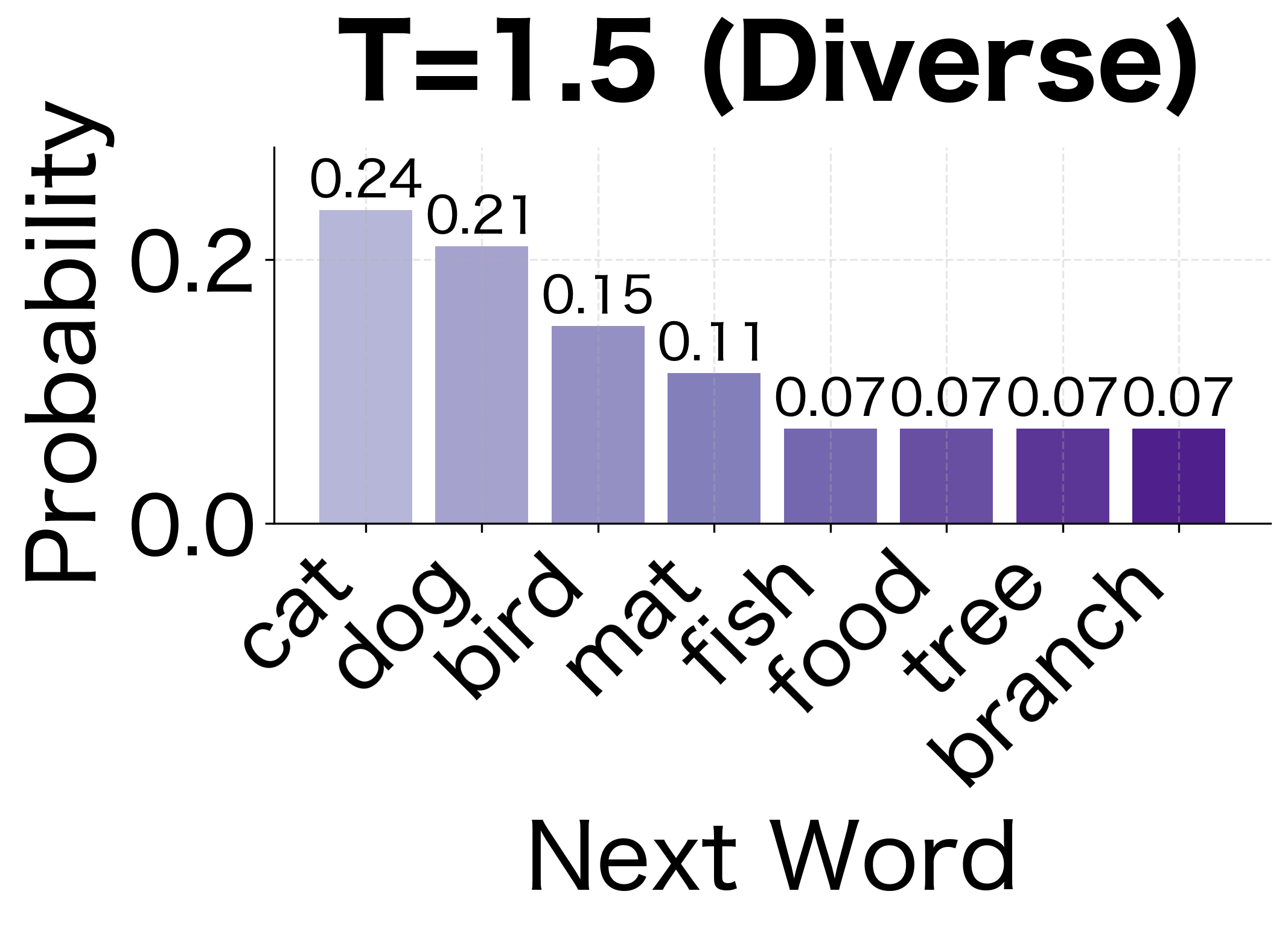
The plots illustrate how temperature reshapes probability distributions. At T=0.5, the highest-probability word dominates the distribution. At T=1.5, the distribution flattens and rare words have a much better chance of being selected. This trade-off between coherence and diversity reappears in transformer-based language models, where it is controlled by exactly the same mechanism.

NLTK provides a well-tested n-gram language modeling module that handles the bookkeeping of counting, vocabulary management, and probability computation:

The NLTK predictions match what we expect from our training data. Given ["the"], the model predicts words like "cat," "dog," and "bird" that frequently follow "the." Given ["sat", "on"], the model strongly predicts "the." NLTK's padded_everygram_pipeline handles the boundary token logic automatically. The MLE class implements the same count-based formula we derived earlier.

The key parameters for n-gram language models are:

• n (n-gram order): Controls how many words of context the model considers. Unigrams ($n=1$) ignore context entirely. Bigrams ($n=2$) use one word of context. Trigrams ($n=3$) were the production standard before neural models. Higher values require exponentially more training data.

• temperature: Controls randomness during text generation. Values below 1.0 make generation more deterministic. Values above 1.0 make generation more diverse. Values between 0.7 and 1.2 work well for most applications.

• start and end tokens: The <s> token provides context for sentence-initial words; prepend $n-1$ start tokens for an order-$n$ model. The </s> token allows the model to learn which words end sentences.

• vocabulary handling: Case normalization reduces vocabulary size but loses capitalization information. An unknown token <UNK> handles out-of-vocabulary words at inference time. A minimum frequency threshold excludes rare words.

Let us walk through the complete process step by step with a concrete example, starting from a raw sentence and ending with a sequence probability. This ties together everything from this chapter.

Setup. Suppose we train a bigram model on the sentence "the cat sat on the mat" (treated as both training and test for illustration). We want to compute the probability of the new sentence "the cat sat on the mat" under the learned model.

Step 1: Tokenize and add markers.

The sentence becomes: <s> the cat sat on the mat </s>

Step 2: Count unigrams.

From "the cat sat on the mat":

• the: 2
• cat: 1
• sat: 1
• on: 1
• mat: 1

Step 3: Count bigrams (with markers).

• <s> the: 1
• the cat: 1
• cat sat: 1
• sat on: 1
• on the: 1
• the mat: 1
• mat </s>: 1

Step 4: Apply MLE formula.

$$P(\text{the}|\text{<s>}) = \frac{C(\text{<s>, the})}{C(\text{<s>})} = \frac{1}{1} = 1.0$$ $$P(\text{cat}|\text{the}) = \frac{C(\text{the, cat})}{C(\text{the})} = \frac{1}{2} = 0.5$$ $$P(\text{sat}|\text{cat}) = \frac{C(\text{cat, sat})}{C(\text{cat})} = \frac{1}{1} = 1.0$$ $$P(\text{on}|\text{sat}) = \frac{C(\text{sat, on})}{C(\text{sat})} = \frac{1}{1} = 1.0$$ $$P(\text{the}|\text{on}) = \frac{C(\text{on, the})}{C(\text{on})} = \frac{1}{1} = 1.0$$ $$P(\text{mat}|\text{the}) = \frac{C(\text{the, mat})}{C(\text{the})} = \frac{1}{2} = 0.5$$ $$P(\text{</s>}|\text{mat}) = \frac{C(\text{mat, </s>})}{C(\text{mat})} = \frac{1}{1} = 1.0$$

Step 5: Multiply the conditional probabilities.

$$\begin{aligned} P(\text{the cat sat on the mat}) &= P(\text{the}|\text{<s>}) \times P(\text{cat}|\text{the}) \\ &\quad \times P(\text{sat}|\text{cat}) \times P(\text{on}|\text{sat}) \\ &\quad \times P(\text{the}|\text{on}) \times P(\text{mat}|\text{the}) \\ &\quad \times P(\text{</s>}|\text{mat}) \\ &= 1.0 \times 0.5 \times 1.0 \times 1.0 \times 1.0 \times 0.5 \times 1.0 \\ &= 0.25 \end{aligned}$$

Step 6: Compute log probability.

$$\log P = \log(1.0) + \log(0.5) + \log(1.0) + \log(1.0) + \log(1.0) + \log(0.5) + \log(1.0)$$ $$= 0 + (-0.693) + 0 + 0 + 0 + (-0.693) + 0 = -1.386$$

Step 7: Compute perplexity.

The sequence has 6 content words plus the end token, so $N = 7$:

$$\text{PP} = \exp\!\left(-\frac{-1.386}{7}\right) = \exp(0.198) \approx 1.219$$

This is remarkably low perplexity, essentially because the model was evaluated on its own training sentence. In real evaluation, we always separate training and test data.

Let us verify this programmatically: