InteractiveInverse Document Frequency: How Rare Words Reveal Document Meaning

Inverse Document FrequencyLink Copied

Term frequency tells you how important a word is within a document. But it says nothing about how important that word is across your entire corpus. The word "learning" appearing 5 times in a document about machine learning is meaningful. The word "the" appearing 5 times is not. Both have the same term frequency, yet one carries far more information.

Inverse Document Frequency (IDF) addresses this gap. It measures how rare or common a word is across all documents, giving higher weights to words that appear in fewer documents. When combined with term frequency, IDF creates TF-IDF, one of the most successful text representations in information retrieval history.

This chapter develops IDF from first principles. You'll learn why rare words matter more, derive the IDF formula, explore smoothing variants that prevent mathematical edge cases, and implement efficient IDF computation. By the end, you'll understand the design choices behind IDF and be ready to combine it with TF in the next chapter.

The Problem with Term Frequency AloneLink Copied

In the previous chapter, we computed term frequency to measure word importance within documents. But TF has a blind spot: it treats all words equally regardless of their corpus-wide distribution.

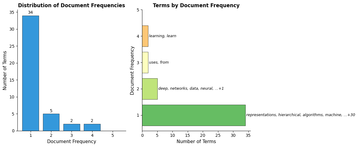
Consider a corpus of research papers about machine learning:

Both "neural" and "from" appear twice in Document 1, giving them equal term frequency. But "neural" is specific to this document's topic, while "from" appears in almost every English text. Term frequency alone cannot distinguish between these cases.

Document Frequency Reveals Corpus-Wide PatternsLink Copied

To understand which words are informative, we need to look beyond individual documents. Document frequency (DF) counts how many documents contain each word:

The pattern emerges clearly. Words like "learning" and "from" appear in most documents, providing little discriminative power. Words like "reinforcement", "vision", and "convolutional" appear in only one document, making them highly specific to particular topics.

The IDF FormulaLink Copied

We've established that document frequency reveals which words are common versus rare across a corpus. But document frequency measures commonality, and what we actually need is a measure of informativeness. The more documents a word appears in, the less useful it is for distinguishing between documents. We need to flip the relationship.

From Commonality to InformativenessLink Copied

Think about what makes a word useful for identifying a document's topic. If someone mentions "convolutional" in a conversation about machine learning papers, you immediately know they're discussing computer vision or deep learning architectures. That single word narrows down the possibilities dramatically. But if they mention "learning", you've learned almost nothing, because every paper in the corpus discusses learning in some form.

This intuition suggests a simple principle: the fewer documents a word appears in, the more informative it is. A word appearing in 1 out of 100 documents carries far more signal than a word appearing in 99 out of 100. We want to assign weights that reflect this inverse relationship.

The most direct approach would be to use the inverse of the document frequency fraction. If a word appears in $\text{df}(t)$ documents out of $N$ total, its "rarity" could be measured as:

This ratio captures the essence of what we want. For a word appearing in just 1 document out of 100, the ratio is 100. For a word appearing in all 100 documents, the ratio is 1. Rare words get high values; common words get low values.

But there's a problem with using this ratio directly.

Why We Need the LogarithmLink Copied

Consider a corpus of 1 million documents. A word appearing once would get weight 1,000,000. A word appearing in half the documents would get weight 2. This 500,000-fold difference is extreme. In practice, it would mean that a single rare word would completely dominate any calculation, drowning out the contribution of all other words.

What we need is a function that preserves the ordering (rare words still get higher weights than common words) but compresses the range of values. The logarithm is the natural choice for this transformation. It converts multiplicative differences into additive ones, turning that 500,000x gap into something more manageable.

With the logarithm, our 1-million-document example becomes:

• Word appearing once: $\log(1,000,000) \approx 13.8$
• Word appearing in 500,000 documents: $\log(2) \approx 0.69$

The ratio is now about 20:1 instead of 500,000:1. Rare words still matter more, but they don't completely overwhelm everything else.

This brings us to the complete IDF formula:

Understanding the Formula's BehaviorLink Copied

Let's trace through what happens at the extremes to build intuition:

When a word appears in every document ($\text{df}(t) = N$):

A word appearing everywhere provides zero discriminative information. This makes sense: if every document contains "the", knowing a document contains "the" tells you nothing about which document it is.

When a word appears in exactly one document ($\text{df}(t) = 1$):

This is the maximum possible IDF value for a given corpus size. Such words are maximally informative because they uniquely identify specific documents.

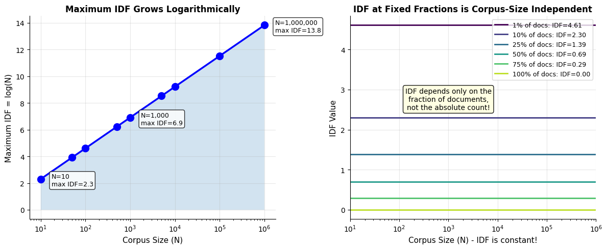
When a word appears in half the documents ($\text{df}(t) = N/2$):

This value is independent of corpus size. A word appearing in half the documents always has the same IDF, whether the corpus has 10 documents or 10 million.

The choice of logarithm base affects the scale of IDF values but not their relative ordering. Natural log (ln), log base 2, and log base 10 are all common choices. scikit-learn uses natural log by default.

Implementing IDF from ScratchLink Copied

Let's translate the formula into code. The implementation is straightforward: for each term, we compute the log of the ratio of total documents to document frequency.

Now let's examine the IDF values for our corpus. We'll display each term alongside its document frequency, the raw ratio $N/\text{df}(t)$, and the final IDF value. This breakdown helps us see how the logarithm transforms the raw ratios.

The output confirms what we predicted. Words appearing in all 5 documents (like "learning" and "from") have IDF = 0, since $\log(5/5) = \log(1) = 0$. Words appearing in only 1 document (like "reinforcement" and "convolutional") achieve the maximum IDF of $\log(5) \approx 1.61$. This range, from 0 to $\log(N)$, is characteristic of IDF.

Visualizing the IDF CurveLink Copied

The relationship between document frequency and IDF is not linear. As document frequency increases, IDF decreases, but the rate of decrease slows down. This logarithmic curve has important implications for how we weight terms.

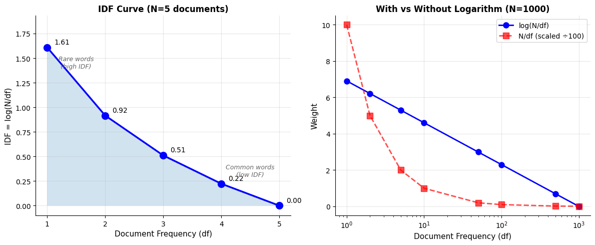
The right panel reveals why the logarithm matters at scale. Without it (red dashed line, scaled down 100x for visibility), the curve is extremely steep, with rare words receiving weights hundreds of times larger than common words. The logarithmic version (blue) provides a gentler gradient that maintains the ordering while keeping weights in a manageable range.

Notice also how the logarithmic curve flattens as document frequency increases. The difference between appearing in 1 document versus 2 documents is much larger than the difference between appearing in 500 versus 1000 documents. This makes intuitive sense: the jump from "unique" to "appears twice" is more significant than the jump from "pretty common" to "slightly more common."

The Information Theory ConnectionLink Copied

We've motivated IDF through intuition about word informativeness, but there's a deeper theoretical foundation. The IDF formula isn't arbitrary; it emerges naturally from information theory.

Surprisal and Information ContentLink Copied

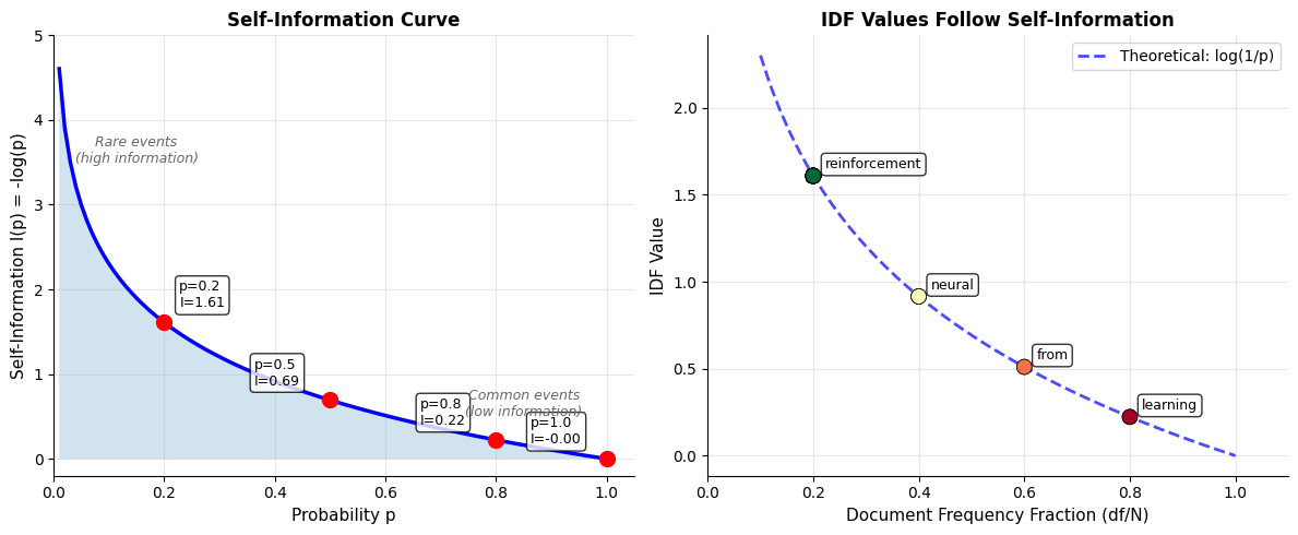
In information theory, the self-information (also called surprisal) of an event measures how surprising or informative that event is. The key insight is that rare events carry more information than common events. If someone tells you "the sun rose this morning," you learn nothing new. If they tell you "there was a solar eclipse this morning," you've learned something significant.

From Probability to IDFLink Copied

Now let's connect this to document frequency. If we treat each document as a random draw from the corpus, we can estimate the probability that a randomly selected document contains term $t$:

This is simply the fraction of documents containing the term. A word appearing in 20 out of 100 documents has an estimated probability of 0.2 of appearing in any given document.

Substituting this probability estimate into the self-information formula:

This derivation shows that IDF is exactly the self-information of a term's occurrence. We're not using an arbitrary weighting scheme; we're measuring the information content of words in a principled way grounded in information theory.

This connection explains why IDF works so well. Information theory tells us that rare events are more informative, and IDF operationalizes this principle for text. When we give higher weights to rare words, we're actually measuring how much information those words convey about document identity.

Let's verify this connection empirically by computing both IDF and self-information independently and comparing the results.

Now we compare the self-information values (computed from probabilities) with the IDF values (computed from document frequencies). If our derivation is correct, they should be identical.

Every term shows a perfect match between self-information and IDF. This isn't a coincidence or approximation; it's a mathematical identity. The IDF formula is the self-information formula, just expressed in terms of document counts rather than probabilities.

Smoothed IDF VariantsLink Copied

The basic IDF formula is elegant, but it has edge cases that cause problems in practice. Understanding these edge cases and their solutions deepens our understanding of how IDF works.

Edge Case 1: Words Appearing EverywhereLink Copied

What happens when a term appears in every document? With $\text{df}(t) = N$:

A word appearing in every document gets zero weight. From a discriminative standpoint, this makes sense: such a word provides no information for distinguishing between documents. But zero weight means the word contributes nothing to any similarity calculation, even if it might carry some semantic meaning.

Edge Case 2: Out-of-Vocabulary TermsLink Copied

A more serious problem arises when processing new documents that contain words not seen during training. If a query contains a word with $\text{df}(t) = 0$, we get:

Division by zero breaks the computation entirely. This out-of-vocabulary (OOV) problem is common in production systems where new documents may contain novel terminology.

Smoothing SolutionsLink Copied

Smoothed IDF variants address these edge cases by adding constants to the formula. Different variants make different trade-offs.

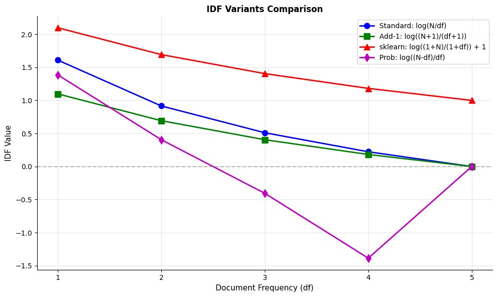
Add-One Smoothing adds 1 to both numerator and denominator:

where $N$ is the total number of documents and $\text{df}(t)$ is the document frequency of term $t$.

This handles the OOV problem: a word with $\text{df}(t) = 0$ gets $\log\left(\frac{N+1}{1}\right) = \log(N+1)$, the maximum possible IDF. However, terms appearing in all documents still get zero: $\log\left(\frac{N+1}{N+1}\right) = 0$.

scikit-learn's Smoothed IDF takes a different approach:

where $N$ is the total number of documents and $\text{df}(t)$ is the document frequency of term $t$.

The +1 added to both numerator and denominator prevents division by zero and provides symmetric smoothing. The +1 added outside the logarithm ensures all terms get positive weights, even those appearing in every document. For a term in all $N$ documents: $\log\left(\frac{1+N}{1+N}\right) + 1 = 1$. This is the default in TfidfVectorizer.

Probabilistic IDF comes from a different theoretical motivation:

where $N$ is the total number of documents and $\text{df}(t)$ is the document frequency of term $t$.

This formula measures the odds ratio of a term being absent versus present. It produces negative weights for terms appearing in more than half the documents (when $\text{df}(t) > N/2$). This treats very common words as anti-discriminative, actively reducing similarity scores when they appear. Some retrieval models use this property intentionally.

Let's implement all four variants and compare their behavior across different document frequencies.

We'll display terms sorted by document frequency (most common first) to see how each variant handles the spectrum from ubiquitous to rare words.

The comparison reveals each variant's character:

• Standard IDF gives exactly 0 to terms appearing in all documents, treating them as completely uninformative.
• Add-1 smoothing slightly reduces all IDF values but still gives 0 to ubiquitous terms.
• sklearn's formula adds a constant offset, ensuring every term gets a positive weight (minimum ~1.0).
• Probabilistic IDF produces negative values for terms in more than half the documents, treating them as anti-discriminative.

IDF Across Corpus SplitsLink Copied

In machine learning, we often split data into training and test sets. How should we handle IDF in this scenario?

The key principle is: compute IDF only on training data, then apply it to test data.

If we compute IDF on the full dataset (including test data), we're leaking information from the test set into our features. This can lead to overly optimistic performance estimates.

When applying IDF to test documents, terms not seen in training get a default IDF value (often the maximum IDF from training, treating unknown words as maximally informative, or zero, treating them as uninformative).

The Vocabulary Mismatch ProblemLink Copied

Test documents may contain words not in the training vocabulary. This out-of-vocabulary (OOV) problem requires a decision:

1. Ignore OOV terms: Simply skip words not in the training vocabulary
2. Assign maximum IDF: Treat unknown words as maximally rare
3. Assign zero IDF: Treat unknown words as uninformative

scikit-learn's TfidfVectorizer uses approach 1 by default: OOV terms are ignored during transformation.

Implementing IDF EfficientlyLink Copied

For large corpora, efficient IDF computation matters. Let's compare a naive implementation with an optimized approach:

The speedup demonstrates why algorithm choice matters. The optimized version makes a single pass through the corpus, using a set to count each term once per document. The naive version iterates through all documents for each vocabulary term, making it $O(V \times D)$ instead of $O(\text{total tokens})$. For production systems with millions of documents and large vocabularies, this difference can mean hours versus seconds of computation time.

Using scikit-learn for ProductionLink Copied

For production systems, use scikit-learn's TfidfVectorizer, which computes IDF efficiently and handles all edge cases:

The values match exactly between scikit-learn's implementation and our manual calculation of the sklearn variant formula. This confirms that TfidfVectorizer with smooth_idf=True uses $\log\left(\frac{1 + N}{1 + \text{df}(t)}\right) + 1$. For production applications, always use scikit-learn rather than implementing IDF manually, as it handles edge cases, optimizes memory usage, and integrates seamlessly with machine learning pipelines.

Visualizing IDF in ActionLink Copied

Let's see how IDF transforms our understanding of word importance. We'll compare raw document frequency with IDF weights:

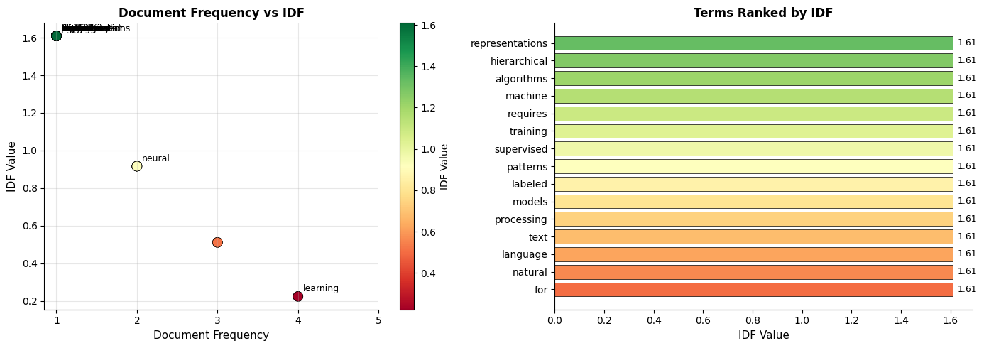
The ranking by IDF reveals which terms are most discriminative. Topic-specific words like "reinforcement", "vision", and "convolutional" rank highest, while common words like "learning" and "from" rank lowest.

IDF Heatmap Across DocumentsLink Copied

Let's visualize how IDF weights apply across our document collection:

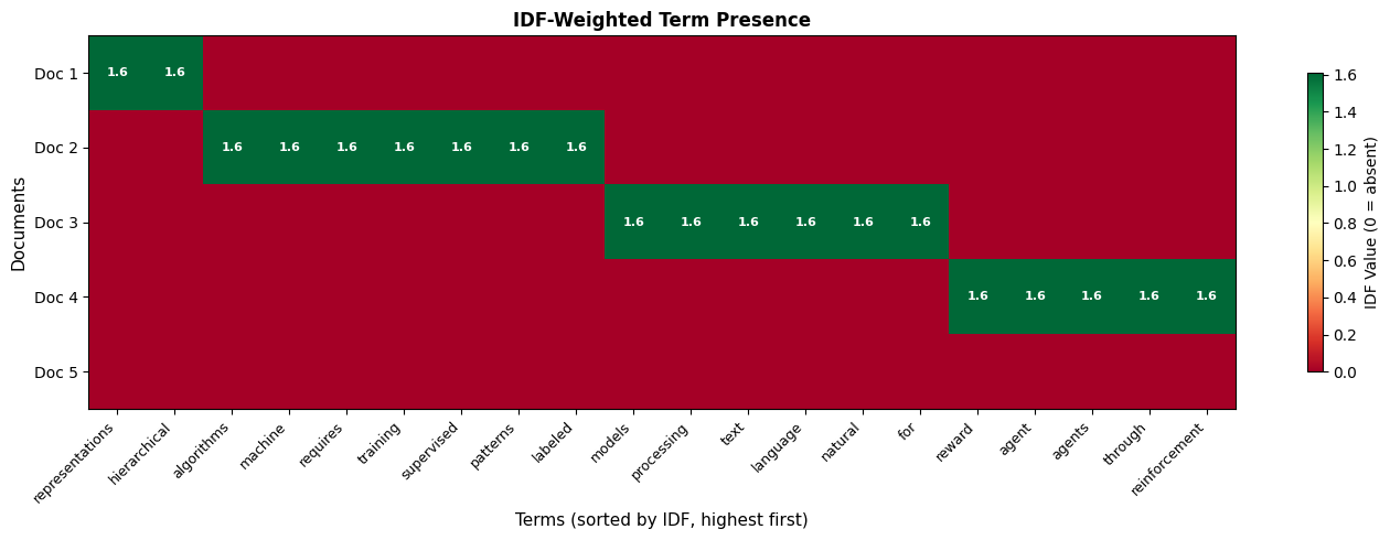
The heatmap reveals document structure. Document 4 is characterized by "reinforcement" and "reward" (high IDF, appearing only there). Document 5 is characterized by "vision", "convolutional", and "image". The common words on the right appear across multiple documents with lower IDF values.

Limitations and ImpactLink Copied

IDF addresses a fundamental limitation of term frequency by incorporating corpus-wide statistics. But it has its own limitations:

Assumes rarity equals importance: IDF treats all rare words as informative. But a typo appearing once is not more informative than a common word. Rare words might be noise, not signal.

Static corpus assumption: IDF weights are computed from a fixed corpus. In streaming applications where new documents arrive continuously, IDF values become stale and may need periodic recomputation.

No semantic understanding: "Good" and "excellent" might have similar IDF values but are treated as completely unrelated. IDF captures statistical patterns, not meaning.

Sensitive to corpus composition: IDF values depend entirely on the corpus. A word rare in one domain might be common in another. Models trained on news articles may not transfer well to scientific papers.

Despite these limitations, IDF was a breakthrough in information retrieval. It provided a principled way to weight terms that dramatically improved search quality. The insight that rare words matter more remains foundational, even as modern systems use more sophisticated approaches.

What IDF UnlockedLink Copied

Before IDF, search systems struggled with the "vocabulary mismatch" problem: queries and documents might use different words for the same concepts. IDF helped by:

1. Downweighting stop words automatically, without requiring a manually curated stop word list
2. Boosting discriminative terms that distinguish relevant from irrelevant documents
3. Enabling relevance ranking by combining TF and IDF into a single score

The TF-IDF combination, which we'll explore in the next chapter, became the standard for text representation in information retrieval for decades. Even modern neural approaches often use TF-IDF as a baseline or component.

SummaryLink Copied

Inverse Document Frequency measures how informative a term is across a corpus by computing the logarithm of the inverse document frequency ratio:

Key insights from this chapter:

• Document frequency counts how many documents contain each term, revealing corpus-wide patterns that term frequency alone cannot capture
• IDF gives higher weights to rare words that appear in few documents, treating them as more informative for distinguishing between documents
• The logarithm compresses the range of weights, preventing rare words from completely dominating common words
• IDF equals self-information from information theory, providing theoretical justification for the formula
• Smoothed variants handle edge cases like terms appearing in all documents or out-of-vocabulary terms
• Train/test splits require computing IDF only on training data to avoid information leakage
• Efficient implementation uses a single pass through the corpus rather than iterating over each term

IDF addresses the key limitation of term frequency: TF treats all words equally regardless of their corpus-wide distribution. By combining TF with IDF, we get TF-IDF, a representation that captures both within-document importance and cross-document discriminative power. The next chapter brings these two components together.

Key Functions and ParametersLink Copied

When working with IDF in scikit-learn, the TfidfVectorizer class handles both TF and IDF computation:

TfidfVectorizer(use_idf, smooth_idf, sublinear_tf, norm)

• use_idf (default: True): Whether to apply IDF weighting. Set to False to compute only term frequency without IDF.

• smooth_idf (default: True): Whether to add 1 to document frequencies to prevent division by zero and ensure all terms get positive IDF values. Uses the formula $\log\left(\frac{1 + N}{1 + \text{df}(t)}\right) + 1$.

• sublinear_tf (default: False): Whether to apply log-scaling to term frequency. When True, uses $1 + \log(\text{tf})$ instead of raw counts.

• norm (default: 'l2'): Normalization applied to output vectors. Use 'l2' for cosine similarity, 'l1' for Manhattan distance, or None for raw TF-IDF values.

The idf_ attribute contains the learned IDF weights after fitting, accessible via vectorizer.idf_.

QuizLink Copied

Ready to test your understanding? Take this quick quiz to reinforce what you've learned about Inverse Document Frequency.