

Master TF-IDF for text representation, including the core formula, variants like log-scaled TF and smoothed IDF, normalization techniques, document similarity with cosine similarity, and BM25 as a modern extension.

This article is part of the free-to-read Language AI Handbook
Choose your expertise level to adjust how many terms are explained. Beginners see more tooltips, experts see fewer to maintain reading flow. Hover over underlined terms for instant definitions.
TF-IDF
You've counted words. You've explored term frequency variants that weight those counts. Now comes the crucial insight: a word's importance depends not just on how often it appears in a document, but on how rare it is across the corpus. The word "the" might appear 50 times in a document, but it tells you nothing because it appears in every document. The word "transformer" appearing just twice might be highly informative if it's rare elsewhere.
TF-IDF, short for Term Frequency-Inverse Document Frequency, combines these two signals into a single score. It's one of the most successful text representations in information retrieval, powering search engines and document similarity systems for decades. The formula is simple: multiply how often a term appears in a document by how rare it is across the corpus. Common words get downweighted; distinctive words get boosted.
This chapter brings together everything from the previous chapters on term frequency and inverse document frequency. You'll learn the exact TF-IDF formula and its variants, implement it from scratch, understand normalization options, and master scikit-learn's TfidfVectorizer. By the end, you'll know when TF-IDF works, when it fails, and how its successor BM25 addresses some of its limitations.
The TF-IDF Formula
This section develops the TF-IDF formula from first principles. We start with the problem of quantifying word importance, then build up each component of the formula step by step, showing how term frequency and inverse document frequency combine to create meaningful document representations.
The Challenge: Quantifying Word Importance
Imagine you're building a search engine for a collection of machine learning papers. When someone searches for "neural networks," you need to rank documents by relevance. But how do you decide which words in each document actually matter for this search?
The problem becomes clear when you look at actual documents. Every paper contains words like "the," "is," "data," and "model" - these appear everywhere and tell you nothing about what makes this paper unique. But other words like "backpropagation," "convolutional," or "transformer" appear much more selectively. Intuitively, you know these rarer, more specific words should carry more weight in determining relevance.
TF-IDF solves this fundamental problem by asking two essential questions about every word in every document:
- How prominent is this word in this specific document? (Local importance)
- How distinctive is this word across the entire collection? (Global rarity)
TF-IDF recognizes that both questions must be answered well for a word to be truly important. A word becomes a strong signal only when it's both prominent locally and distinctive globally.
From Intuition to Mathematics: Building the Formula
Let's develop the TF-IDF formula step by step, understanding why each mathematical choice addresses a specific aspect of the word importance problem.
Step 1: Capturing Local Prominence with Term Frequency
The most straightforward way to measure a word's importance to a document is simply counting how often it appears. If "neural" appears 5 times in a paper about neural networks while "algorithm" appears only once, it's reasonable to conclude that "neural" is more central to this document's content.
This intuition leads to the term frequency (TF):
where:
- : the term (word) whose frequency we're measuring
- : the document we're examining
- : the raw count of how many times term appears in document
Raw term frequency captures the local prominence we want, but it has a critical weakness. Consider a document where "the" appears 50 times, "neural" appears 5 times, and "backpropagation" appears 3 times. The raw counts suggest "the" is most important, which is clearly wrong. We need a way to distinguish between ubiquitous function words and meaningful content words.
Step 2: Capturing Global Distinctiveness with Inverse Document Frequency
To identify words that truly distinguish documents from each other, we need to look across the entire corpus. A word that appears in every document (like "the" or "data") is useless for distinguishing between them. But a word that appears in only a few documents (like "backpropagation" or "transformer") is highly distinctive.
This leads us to document frequency - counting how many documents contain each term:
where:
- : the term whose document frequency we're computing
- : the corpus (collection of all documents)
- : a document in the corpus
- : indicates that term appears at least once in document
- : denotes the count (cardinality) of the set
In plain terms, counts how many documents in the corpus contain the term at least once.
The key insight is that we want to reward rarity, not frequency. Rare words should score high, common words should score low. We achieve this by inverting the relationship through the logarithm:
where:
- : the term whose inverse document frequency we're computing
- : the corpus (collection of all documents)
- : the total number of documents in corpus (i.e., )
- : the document frequency of term (how many documents contain )
- : the natural logarithm (base )
The fraction represents the inverse of the proportion of documents containing term . Rare terms have small , making this fraction large. Common terms have large , making the fraction approach 1.
Why the logarithm? It serves two crucial purposes:
- Inversion: Rare words (low document frequency) get high IDF scores, common words (high document frequency) get low scores
- Scale compression: A word appearing in 1 of 1000 documents doesn't get 1000× the weight of a word appearing in 100 documents. The logarithmic scale ensures that differences in commonness are meaningful but not overwhelming.
Consider three words in a 1000-document corpus:
- "the" appears in 1000 documents: IDF = log(1000/1000) = log(1) = 0
- "neural" appears in 100 documents: IDF = log(1000/100) = log(10) ≈ 2.3
- "backpropagation" appears in 1 document: IDF = log(1000/1) = log(1000) ≈ 6.9
The progression makes intuitive sense: "the" gets no boost, "neural" gets a moderate boost, and "backpropagation" gets a substantial boost.
The logarithmic transformation creates a natural hierarchy that matches our intuition about word distinctiveness. To see this more clearly, let's visualize how IDF scores change as words become more or less common across a corpus.
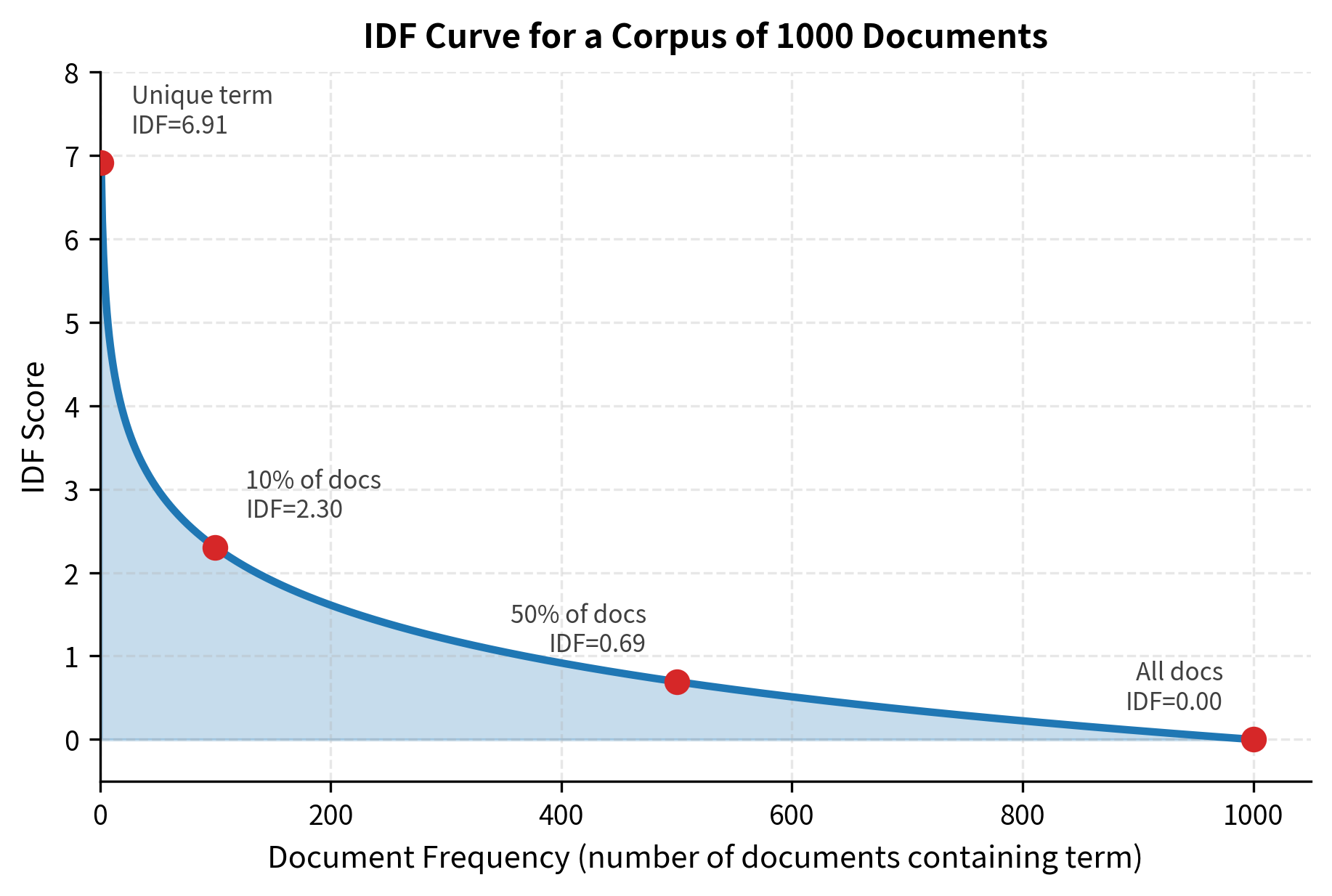
This curve illustrates why logarithmic scaling is essential. Without it, the difference between a word appearing in 1 vs 10 documents would be the same as the difference between appearing in 990 vs 1000 documents - clearly not what we want.
Step 3: The Crucial Synthesis - Multiplying TF and IDF
Now we have two complementary perspectives on word importance:
- Term Frequency (TF): Captures local prominence within a document
- Inverse Document Frequency (IDF): Captures global distinctiveness across the corpus
The question is: how do we combine these signals? The answer reveals the core insight of TF-IDF.
Consider what happens with different combinations of TF and IDF:
- High TF, Low IDF (like "the" appearing 50 times): This word dominates locally but is ubiquitous globally. We want to heavily penalize it.
- Low TF, High IDF (like "backpropagation" appearing once): This word is distinctive globally but not prominent locally. It shouldn't dominate the document's representation.
- High TF, High IDF (like "neural" appearing 5 times in a neural networks paper): This word is both prominent locally and distinctive globally. This is exactly what we want to reward.
Multiplication naturally creates this behavior. When you multiply TF and IDF:
- High TF × Low IDF = Moderate score (common words get downweighted)
- Low TF × High IDF = Moderate score (rare words alone aren't enough)
- High TF × High IDF = High score (the sweet spot we want)
This multiplicative synthesis leads to the complete TF-IDF formula:
TF-IDF combines term frequency and inverse document frequency through multiplication:
where:
- is a term (word)
- is a document
- is the corpus (collection of all documents)
- measures local prominence (how often appears in )
- measures global distinctiveness (how rare is across )
The multiplication ensures that only words that excel at both local prominence and global distinctiveness achieve high TF-IDF scores. This creates a representation where each document is characterized by its most unique and relevant terms.
Bringing the Theory to Life: Implementing TF-IDF
Now that we understand the mathematical foundation of TF-IDF, let's see how these concepts work in practice. We'll implement the formula step by step on a real corpus, watching how the theory translates into concrete results that reveal the distinctive character of each document.
Our implementation will mirror the conceptual journey we just took - from measuring local prominence (TF) to assessing global distinctiveness (IDF) to combining them through multiplication. This hands-on approach will help you see why each mathematical choice matters and how the formula solves the word importance problem.
Step 1: Setting Up Our Corpus and Basic Functions
Let's start with a small but diverse corpus that covers different areas of machine learning. This will help us see how TF-IDF distinguishes between documents on different topics.
Now let's implement the core functions that capture our two fundamental signals: local prominence (TF) and global distinctiveness (IDF).
Step 2: Examining Global Distinctiveness Through IDF
Let's examine how IDF scores reflect each term's discriminative power across our corpus. We'll look at terms that span the full spectrum from ubiquitous to unique.
The Spectrum of Distinctiveness
The table reveals how IDF creates a natural hierarchy of word importance based on global rarity:
- Ubiquitous terms like "learning" (appears in 4/5 documents, IDF = 0.22) get minimal weight. These words appear everywhere and provide no discriminative signal.
- Moderately distinctive terms like "deep" and "neural" (2/5 documents, IDF = 0.92) receive moderate amplification. They're informative but not unique.
- Highly distinctive terms like "images" and "rewards" (1/5 documents, IDF = 1.61) get the strongest boost. Finding these words in a document immediately tells you something specific about its content and domain.
This solves our original problem: IDF automatically identifies which words distinguish documents from each other, suppressing generic terms while amplifying domain-specific ones.
Step 3: The Synthesis - Computing TF-IDF Scores
Now comes the crucial moment: combining our two signals through multiplication. This is where the theory becomes practice, where local prominence meets global distinctiveness to create a truly informative document representation.
Step 4: Seeing the Results - How TF-IDF Transforms Document Representation
Let's examine how TF-IDF transforms Document 1 (about machine learning algorithms). We'll see the raw components alongside the final scores to understand how the multiplication creates meaningful rankings.
The Transformation in Action
The TF-IDF scores reveal how multiplication balances local and global signals:
-
"Learning" (TF=3, IDF=0.22, TF×IDF=0.67): Despite being the most frequent word in Document 1, its ubiquity across the corpus suppresses its score. This prevents common words from dominating representations.
-
"Data" (TF=2, IDF=0.51, TF×IDF=1.02): A nice balance - moderately frequent locally and moderately distinctive globally. The multiplication finds this sweet spot.
-
"Algorithms" and "Powerful" (TF=1, IDF=1.61, TF×IDF=1.61): These terms appear only once but are unique to this document. Their global rarity compensates for their local scarcity, earning them top scores.
The result is a representation that captures what makes Document 1 distinctive: not just what words it contains, but which words make it different from other documents. TF-IDF has transformed raw frequency counts into meaningful importance scores that reflect both local relevance and global informativeness.
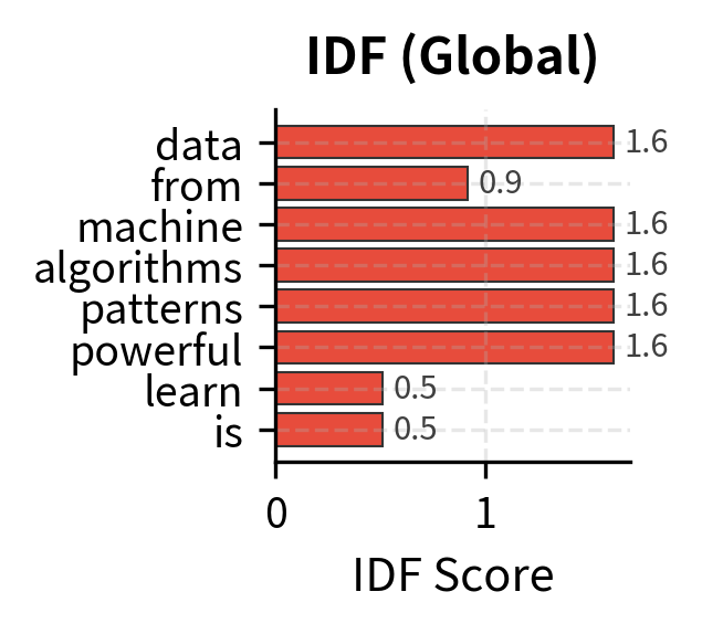
Step 5: Visualizing the Balance - How TF and IDF Work Together
To truly understand how TF-IDF creates meaningful document representations, let's visualize the interplay between local prominence and global distinctiveness. The visualization below decomposes the TF-IDF scores for Document 1, showing how the multiplication of TF and IDF produces rankings that reflect true importance rather than raw frequency.
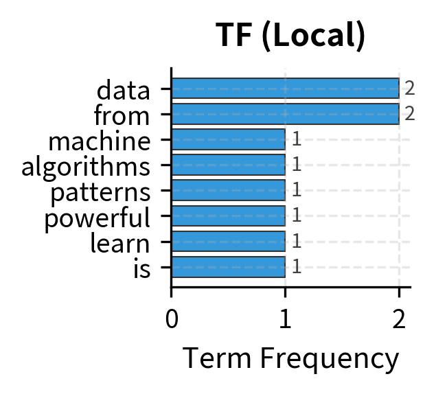
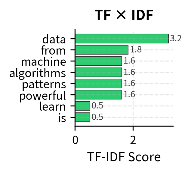
The Complete Picture: From Intuition to Implementation
Our journey through TF-IDF implementation has revealed how the formula transforms raw text into meaningful representations. We started with a fundamental insight - that word importance depends on both local prominence and global distinctiveness - and built a complete system that operationalizes this intuition.
The visualization above captures the essence of TF-IDF: it's not about counting words, but about understanding their significance. Terms like "learning" contribute less than their frequency suggests because they're commonplace. Terms like "algorithms" contribute more than their frequency suggests because they're distinctive.
This multiplicative synthesis creates document representations that truly capture what makes each text unique. TF-IDF doesn't just count words - it measures their discriminative power, creating a foundation for all the text analysis techniques that follow.
TF-IDF Variants
The basic TF-IDF formula we've developed works well, but practitioners have discovered that certain modifications can improve performance for specific tasks. These variants address subtle issues with the basic formulation, issues that become apparent when you think carefully about what the formula is measuring.
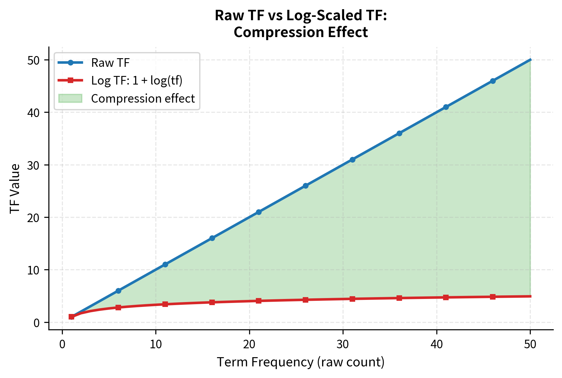
Log-Scaled TF: Taming Extreme Frequencies
Consider a document where "machine" appears 20 times and "learning" appears twice. Is "machine" really 10× more important to this document? Probably not. The relationship between word frequency and importance isn't linear. The first few occurrences establish a word's relevance, but additional occurrences provide diminishing returns.
Log-scaling addresses this proportionality problem by applying a logarithmic transformation:
where:
- : the term whose log-scaled frequency we're computing
- : the document being analyzed
- : the raw term frequency (count of in )
- : the natural logarithm (base )
The "+1" ensures that a term appearing once gets a score of 1 rather than 0 (since ). This preserves the distinction between presence and absence while compressing differences among frequently occurring terms.
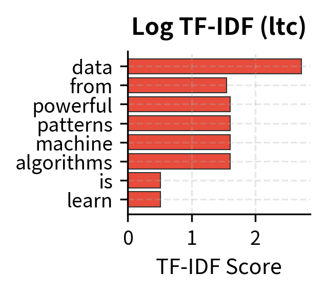
Interpreting the Log-Scaled Results
Log-scaling compresses the TF component, reducing the dominance of high-frequency terms. "Learning" with TF=3 gets log TF of 2.1, not 3. The difference between 3 and 1 occurrence shrinks from 3× to about 2×. This compression is often preferable for document similarity calculations, where you want to recognize that a document mentioning "neural" twice is similar to one mentioning it five times.
Smoothed IDF: Handling Edge Cases
The basic IDF formula has a subtle problem: what happens when a term appears in every document? The formula gives:
A term appearing everywhere gets IDF of zero, which means its TF-IDF is also zero. It contributes nothing to the document representation. While this makes sense for truly universal terms like "the", it can be problematic when you want even common terms to contribute something.
Smoothed IDF variants address this by adding constants to both the numerator and denominator:
where:
- : the term whose smoothed IDF we're computing
- : the corpus
- : the total number of documents in the corpus
- : the document frequency of term
The smoothing modifications serve specific purposes:
- "+1" in the numerator: Ensures the fraction remains well-defined even for edge cases
- "+1" in the denominator: Prevents division by zero for unseen terms (where )
- "+1" added at the end: Shifts all IDF values up, ensuring even terms appearing in every document have positive IDF
This ensures all terms have positive IDF, which is important when you want common words to contribute something rather than nothing.
Why Smoothing Matters
The smoothed version adds a constant offset, ensuring even the most common terms retain some weight. The "+1" in the numerator and denominator prevents division issues with unseen terms, while the final "+1" shifts all IDF values up. This is the default in scikit-learn's TfidfVectorizer, making it important to understand when comparing implementations.
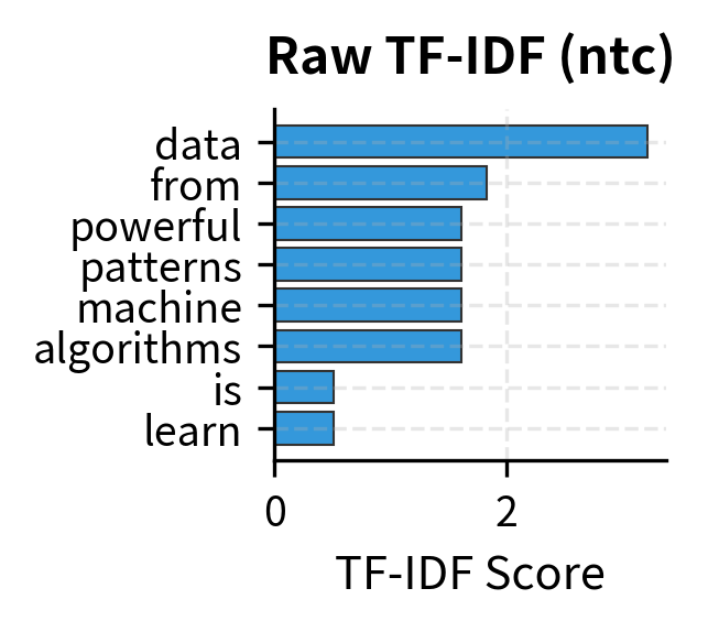
Common TF-IDF Schemes: A Notation System
The information retrieval community developed a compact notation for describing TF-IDF variants. Each scheme is specified by three letters indicating the TF variant, IDF variant, and normalization method. For example, ltc means: log TF, standard IDF, cosine normalization.
Here are the most common schemes and when to use them:
| Scheme | TF | IDF | Normalization | Use Case |
|---|---|---|---|---|
nnn | Raw | None | None | Baseline, raw counts |
ntc | Raw | Standard | Cosine | Basic TF-IDF |
ltc | Log | Standard | Cosine | Balanced weighting |
lnc | Log | None | Cosine | TF only, normalized |
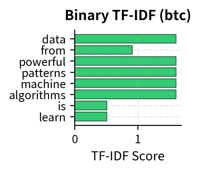
bnn | Binary | None | None | Presence/absence |
TF-IDF Vector Computation
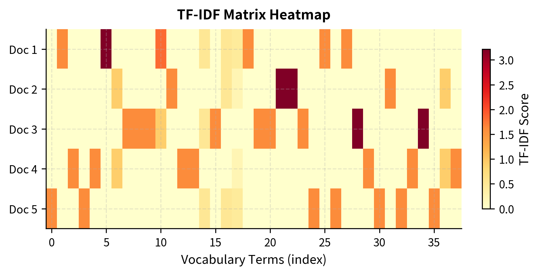
To use TF-IDF for machine learning, we need to convert documents into fixed-length vectors. Each dimension corresponds to a vocabulary term, and the value is that term's TF-IDF score.
Sparsity in TF-IDF Matrices
Like raw count matrices, TF-IDF matrices are extremely sparse. Most documents use only a small fraction of the vocabulary.
TF-IDF Normalization
Raw TF-IDF vectors have varying lengths depending on document size and vocabulary overlap. For similarity calculations, we typically normalize vectors so that document length doesn't dominate.
L2 Normalization
L2 normalization (also called Euclidean normalization) divides each vector by its Euclidean length, projecting all documents onto the unit sphere:
where:
- : the original TF-IDF vector with components
- : the normalized vector
- : the L2 norm (Euclidean length) of vector
- : the sum of squared components, which equals the squared length
- : index over all vocabulary terms (dimensions of the vector)
The result is a unit vector: a vector with length exactly 1.0. After L2 normalization, cosine similarity becomes a simple dot product.
All normalized vectors now have unit length (1.0), making them directly comparable regardless of original document length.
L1 Normalization
L1 normalization (also called Manhattan normalization) divides by the sum of absolute values, making each vector's components sum to 1:
where:
- : the original TF-IDF vector with components
- : the L1-normalized vector
- : the L1 norm (sum of absolute values)
- : the absolute value of the -th component
- : the total "mass" of the vector
After L1 normalization, all components sum to 1, creating a probability-like distribution over terms.
L1 normalization is useful when you want to interpret TF-IDF scores as term "importance proportions" within a document.
Document Similarity with TF-IDF
TF-IDF's primary application is measuring document similarity. Documents with similar TF-IDF vectors discuss similar topics using similar vocabulary.
Cosine Similarity
Cosine similarity measures the angle between two vectors, producing a score that ranges from 0 (orthogonal, completely dissimilar) to 1 (identical direction, maximally similar):
where:
- : the first document's TF-IDF vector
- : the second document's TF-IDF vector
- : the dot product, computed as
- : the L2 norm (Euclidean length) of vector
- : the L2 norm of vector
The numerator captures how much the vectors "point in the same direction" (shared vocabulary with similar weights), while the denominator normalizes for vector length. For L2-normalized vectors (where ), this simplifies to a dot product: .
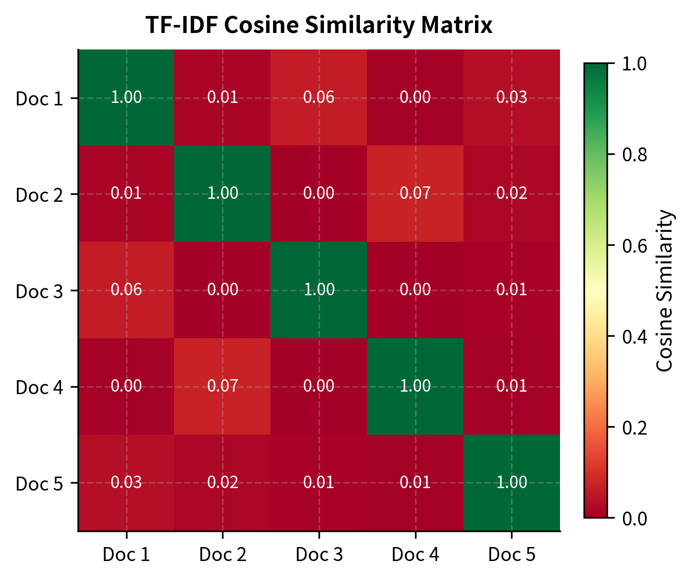
Documents 1 and 5 show moderate similarity (0.28) because both discuss "learning". Documents 2 and 4 share "deep learning" terminology. The diagonal shows perfect self-similarity (1.0).
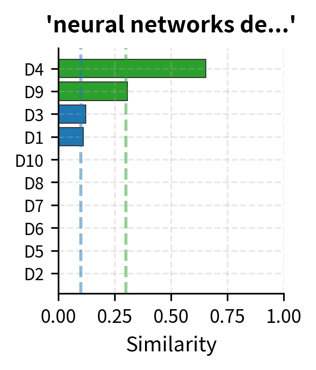
Finding Similar Documents
Given a query document, we can rank all corpus documents by similarity:
Document 4 (Computer Vision) ranks highest because it shares "deep learning" vocabulary with Document 2. Document 1 (Machine Learning) comes second due to shared "learning" terminology.
Visualizing Document Similarity in 2D
While the similarity matrix shows pairwise relationships, we can also visualize how documents cluster in a 2D space. Using PCA to reduce our high-dimensional TF-IDF vectors to 2 dimensions reveals the underlying structure:
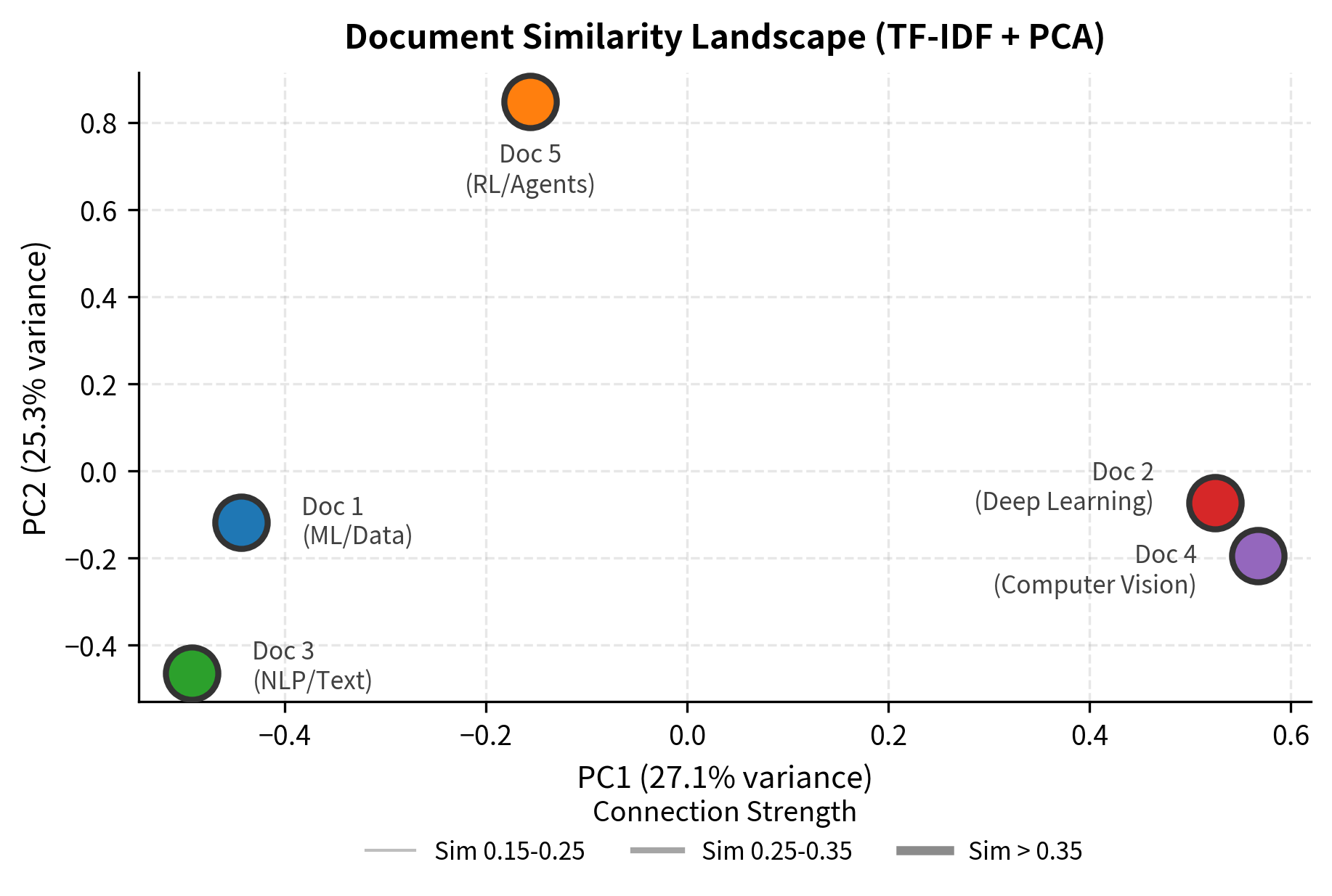
The 2D projection reveals document relationships at a glance. Documents sharing vocabulary (like the "learning"-related documents) appear closer together, while Document 3 (focused on text/NLP) sits farther from the others due to its distinct vocabulary.
TF-IDF for Feature Extraction
Beyond document similarity, TF-IDF vectors serve as features for machine learning models. Text classification, clustering, and information retrieval all benefit from TF-IDF representations.
Text Classification Example
Let's use TF-IDF features for a simple classification task:
TF-IDF features capture the distinctive vocabulary of each class. ML documents contain "learning", "data", "models"; literature documents contain "poetry", "stories", "narrative".
Feature Selection with TF-IDF
High TF-IDF scores identify distinctive terms that can serve as features:
Each document's top TF-IDF terms capture its distinctive content. Document 2's top terms include "neural" and "networks"; Document 3's include "text" and "nlp".
sklearn TfidfVectorizer Deep Dive
scikit-learn's TfidfVectorizer is the standard tool for TF-IDF computation. Understanding its parameters helps you tune it for your specific use case.
Basic Usage
Key Parameters
TfidfVectorizer combines tokenization, TF-IDF computation, and normalization. Here are the most important parameters:
Key observations:
- no_idf: Without IDF, all terms are weighted by frequency alone
- sublinear_tf: Log-scaling compresses TF values
- no_norm: Without normalization, vector norms vary by document length
- bigrams: Including bigrams dramatically increases vocabulary size
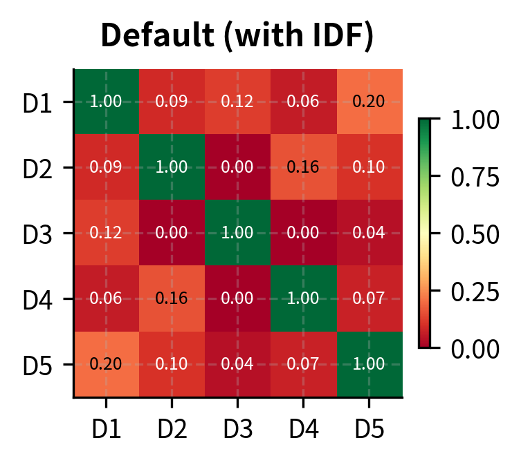
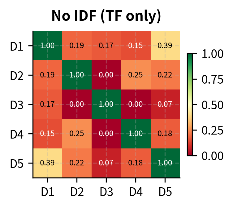
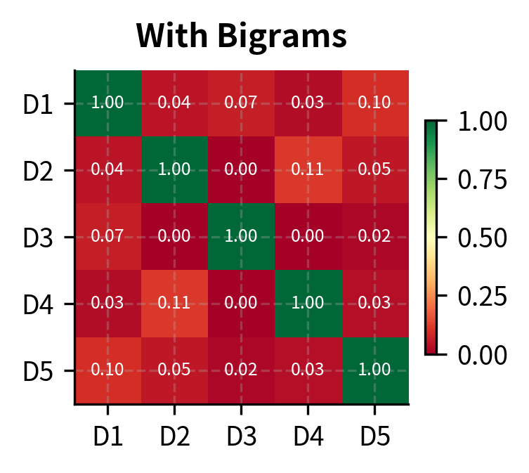
The visualization reveals how configuration choices affect similarity calculations. Without IDF, documents appear more similar because common words aren't downweighted. Bigrams can capture different relationships by considering word pairs like "deep learning" or "neural networks" as single features.
The IDF Formula in sklearn
scikit-learn uses a smoothed IDF formula by default, which differs slightly from the standard textbook formula:
where:
- : the term whose IDF we're computing
- : the total number of documents in the corpus
- : the document frequency of term (number of documents containing )
This smoothed version ensures that even terms appearing in every document receive a positive IDF score (rather than zero), and prevents division-by-zero errors for terms not seen during training.
Practical Configuration Patterns
Different tasks call for different configurations:
Each configuration targets a specific use case:
- Document Similarity: L2 normalization enables direct cosine similarity computation, while log-scaled TF prevents high-frequency terms from dominating. Filtering via
min_dfandmax_dfremoves noise from rare typos and ubiquitous stopwords. - Text Classification: Bigrams capture phrase-level patterns that unigrams miss (like "not good" vs "good"). Limiting vocabulary with
max_featuresprevents overfitting and speeds up training. - Keyword Extraction: Disabling normalization preserves interpretable scores. The highest values directly indicate the most distinctive terms without length adjustment.
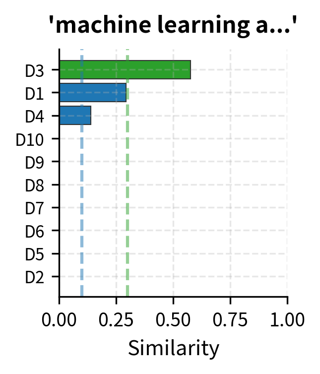
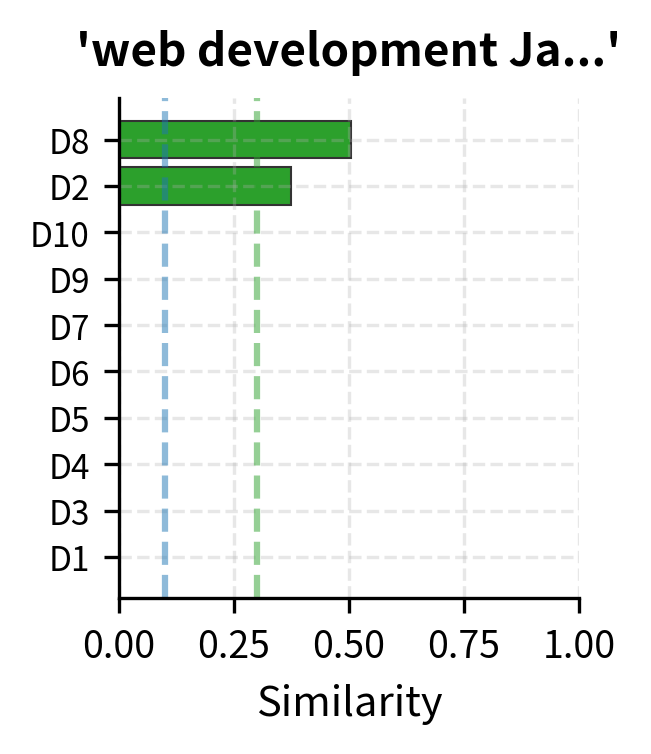
Worked Example: Document Search
Let's build a complete document search system using TF-IDF:
The search system finds relevant documents by matching query terms against the TF-IDF index. "Machine learning algorithms" matches documents about ML and data science. "Web development JavaScript" finds the JavaScript and web development documents.
BM25: TF-IDF's Successor
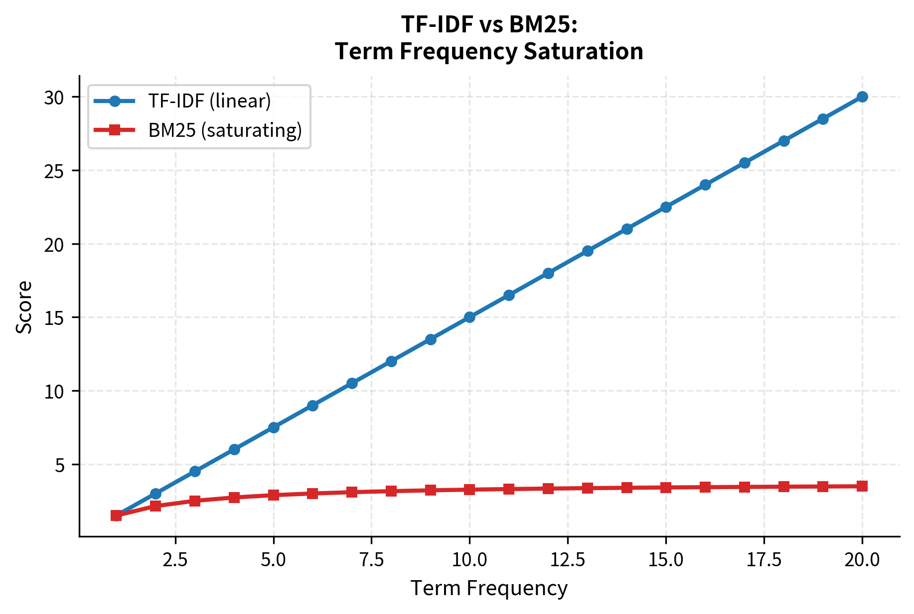
TF-IDF has a limitation: it doesn't handle document length well. A long document naturally has more term occurrences, potentially inflating its relevance scores. BM25 (Best Matching 25) extends TF-IDF with length normalization and saturation.
BM25 is a ranking function that extends TF-IDF with two key improvements:
- Term frequency saturation: Additional occurrences contribute diminishing returns
- Document length normalization: Longer documents are penalized
The formula is:
where:
- : the query term being scored
- : the document being evaluated
- : the corpus
- : the raw term frequency of in document
- : the inverse document frequency of term
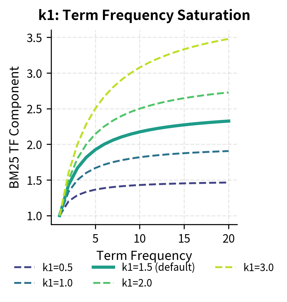
- : saturation parameter controlling how quickly TF saturates (typically 1.2-2.0; higher values mean TF matters more)
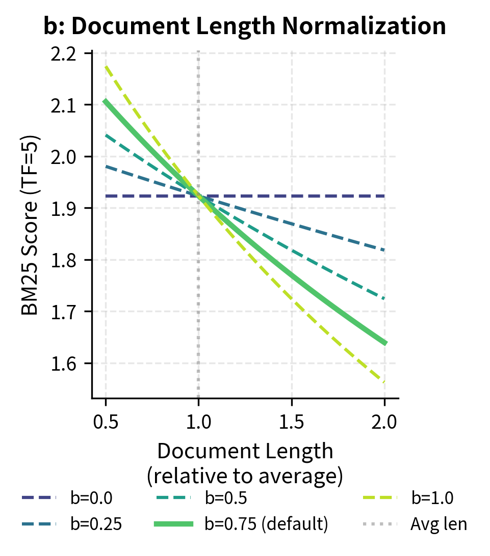
- : length normalization parameter (typically 0.75; 0 = no normalization, 1 = full normalization)
- : the length of document (typically word count)
- : the average document length across the corpus
The term is the length normalization factor. When , this factor equals 1. Longer documents get larger factors (reducing their scores), while shorter documents get smaller factors (boosting their scores).
BM25 Length Normalization
BM25's length normalization adjusts scores based on document length relative to the corpus average:
The following table shows how BM25 scores change with document length, demonstrating the length normalization effect:
Shorter documents get higher BM25 scores for the same term frequency, reflecting the intuition that finding a term in a short document is more significant than finding it in a long one. A term appearing 5 times in a 50-word document is much more dominant than the same 5 occurrences in a 400-word document.
BM25 Parameter Sensitivity
The two key BM25 parameters, and , control different aspects of the scoring:
Using BM25 in Practice
The rank_bm25 library provides a production-ready BM25 implementation:
Limitations and Impact
TF-IDF revolutionized information retrieval and remains widely used, but it has fundamental limitations:
- No semantic understanding: "Car" and "automobile" are treated as completely unrelated terms. TF-IDF cannot capture synonymy, antonymy, or any semantic relationships.
- Vocabulary mismatch: If a query uses different words than the documents (even with the same meaning), TF-IDF will miss the match. "Python programming" won't match "coding in Python" well.
- Bag of words assumption: Like its foundation, TF-IDF ignores word order. "The cat ate the mouse" and "The mouse ate the cat" have identical representations.
- No context: The same word always gets the same IDF, regardless of context. "Bank" (financial) and "bank" (river) are conflated.
- Sparse representations: TF-IDF vectors are high-dimensional and sparse, making them inefficient for neural networks that prefer dense inputs.
Despite these limitations, TF-IDF's impact has been enormous:
- Search engines: Google's early algorithms built on TF-IDF concepts
- Document clustering: K-means on TF-IDF vectors groups similar documents
- Text classification: TF-IDF features power spam filters, sentiment analyzers, and topic classifiers
- Keyword extraction: High TF-IDF terms identify document topics
- Baseline models: TF-IDF provides a strong baseline that neural models must beat
TF-IDF's success comes from its effective balance: it rewards terms that are distinctive to a document while penalizing terms that appear everywhere. This simple idea, implemented efficiently, solved real problems at scale.
Summary
TF-IDF combines term frequency and inverse document frequency to score a term's importance in a document relative to a corpus. The key insights:
- TF-IDF formula:
- TF variants: Raw counts, log-scaled (), binary, and augmented
- IDF variants: Standard (), smoothed ()
- Normalization: L2 normalization enables cosine similarity as a dot product
- Document similarity: Cosine similarity on TF-IDF vectors measures topical overlap
- BM25: Extends TF-IDF with term frequency saturation and document length normalization
TF-IDF remains a powerful baseline for information retrieval and text classification. Its limitations, particularly the lack of semantic understanding, motivated the development of word embeddings and transformer models. But understanding TF-IDF is essential: it's the foundation that modern NLP builds upon.
Key Functions and Parameters
When working with TF-IDF in scikit-learn, TfidfVectorizer is the primary tool:
TfidfVectorizer(lowercase, min_df, max_df, use_idf, norm, sublinear_tf, ngram_range, max_features)
lowercase(default:True): Convert text to lowercase before tokenization.min_df: Minimum document frequency. Integer for absolute count, float for proportion. Usemin_df=2to remove rare terms.max_df: Maximum document frequency. Usemax_df=0.95to filter extremely common terms.use_idf(default:True): Enable IDF weighting. Set toFalsefor TF-only vectors.norm(default:'l2'): Vector normalization. Use'l2'for cosine similarity,'l1'for Manhattan,Nonefor raw scores.sublinear_tf(default:False): Apply log-scaling to TF: replaces tf with .ngram_range(default:(1, 1)): Include n-grams. Use(1, 2)for unigrams and bigrams.max_features: Limit vocabulary to top N terms by corpus frequency.smooth_idf(default:True): Add 1 to document frequencies to prevent zero IDF.
For BM25, use the rank_bm25 library:
BM25Okapi(corpus, k1=1.5, b=0.75)
corpus: List of tokenized documents (list of lists of strings)k1: Term frequency saturation parameter. Higher values give more weight to term frequency.b: Length normalization parameter. 0 disables length normalization; 1 gives full normalization.
Quiz
Ready to test your understanding? Take this quick quiz to reinforce what you've learned about TF-IDF and document representation.

Comments