The Distributional Hypothesis: How Context Reveals Word Meaning

Michael BrenndoerferUpdated March 31, 202539 min read

Learn how the distributional hypothesis uses word co-occurrence patterns to represent meaning computationally, from Firth's linguistic insight to co-occurrence matrices and cosine similarity.

Reading Level

Choose your expertise level to adjust how many terms are explained. Beginners see more tooltips, experts see fewer to maintain reading flow. Hover over underlined terms for instant definitions.

The Distributional Hypothesis

How do children learn what words mean? They don't consult dictionaries. Instead, they observe words in context, gradually building intuitions about meaning from patterns of usage. The word "dog" appears near "bark," "leash," "pet," and "walk." The word "cat" appears near "meow," "purr," "pet," and "scratch." Through exposure, the brain learns that "dog" and "cat" are related (both are pets) yet distinct (different sounds, different behaviors).

This insight, that meaning emerges from patterns of usage, forms the foundation of distributional semantics. The distributional hypothesis proposes that words appearing in similar contexts have similar meanings. This chapter explores this idea from its linguistic origins to its mathematical formalization, showing how it changed the way computers understand language.

Firth's Insight: You Shall Know a Word by the Company It Keeps

In 1957, British linguist J.R. Firth expressed an idea that would influence computational linguistics for decades: "You shall know a word by the company it keeps." This simple phrase captures the essence of the distributional hypothesis.

The Distributional Hypothesis

The distributional hypothesis states that words occurring in similar linguistic contexts tend to have similar meanings. The more often two words appear in the same contexts, the more semantically similar they are likely to be.

Consider the word "oculist." Most people don't know this word. But if you saw it used in sentences like:

  • "I went to the oculist for my annual checkup"
  • "The oculist prescribed new glasses"
  • "My oculist recommended eye drops"

You'd quickly infer that an oculist is some kind of eye doctor. You learned the meaning not from a definition, but from the company the word keeps. The contexts reveal the semantic neighborhood.

In[2]:
Code
# Simulating how context reveals meaning
oculist_contexts = [
    "I visited the ___ to check my vision",
    "The ___ examined my eyes carefully",
    "My ___ recommended new reading glasses",
    "The ___ dilated my pupils for the exam",
]

optometrist_contexts = [
    "I visited the ___ to check my vision",
    "The ___ examined my eyes carefully",
    "My ___ recommended new reading glasses",
    "The ___ dilated my pupils for the exam",
]

# Count shared contexts
shared = len(set(oculist_contexts) & set(optometrist_contexts))
total = len(set(oculist_contexts) | set(optometrist_contexts))
Out[3]:
Console
Context Similarity Analysis:
--------------------------------------------------
'oculist' contexts:     4
'optometrist' contexts: 4
Shared contexts:        4
Context overlap:        100%

The 100% context overlap demonstrates why these two words must have similar meanings. Both "oculist" and "optometrist" fit identically into vision-related sentence patterns, revealing that they occupy the same semantic role despite being different lexical items. This is the distributional hypothesis in action: Words that can substitute for each other in sentences, filling the same "slots," tend to mean similar things.

The Linguistic Foundation

The distributional hypothesis didn't emerge from computer science. It grew from structural linguistics, where researchers noticed that word meaning could be inferred from distributional patterns alone.

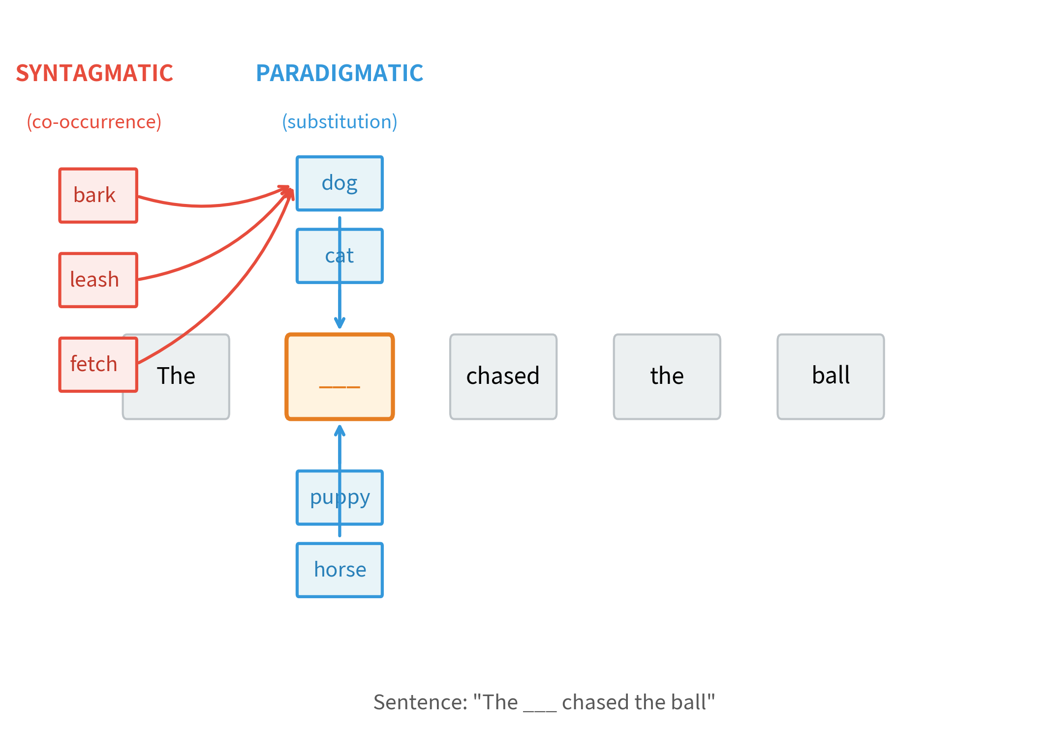
Paradigmatic and Syntagmatic Relations

Linguists distinguish two types of relationships between words:

Paradigmatic Relations

Paradigmatic relations hold between words that can substitute for each other in the same position within a sentence. Words in a paradigmatic relationship belong to the same grammatical category and often share semantic properties. Examples: "cat" and "dog" in "The ___ slept."

Syntagmatic Relations

Syntagmatic relations hold between words that frequently co-occur in sequence or proximity. These relationships reflect how words combine to form meaningful phrases. Examples: "drink" and "coffee," "strong" and "tea."

In[4]:
Code
# Demonstrating paradigmatic vs syntagmatic relations
sentence_template = "The ___ chased the ball"

# Paradigmatic substitutes (can fill the same slot)
paradigmatic_words = ["dog", "cat", "puppy", "kitten", "terrier"]

# Syntagmatic associates (co-occur with "dog")
syntagmatic_words = ["bark", "leash", "fetch", "collar", "walk"]


# Test which words fit the template grammatically
def fits_template(word, template):
    """Check if word fits grammatically (simple heuristic)."""
    return word[0].islower() and len(word) > 2
Out[5]:
Console
Paradigmatic Relations (substitution):
  Template: 'The ___ chased the ball'
  Words that fit: ['dog', 'cat', 'puppy', 'kitten', 'terrier']

Syntagmatic Relations (co-occurrence):
  'dog' frequently appears near: ['bark', 'leash', 'fetch', 'collar', 'walk']

The paradigmatic words all share a common role: they can grammatically fill the subject slot in the template sentence. Meanwhile, the syntagmatic associates frequently appear near the word "dog" but wouldn't substitute for it grammatically. Both types of relations contribute to distributional similarity: Words with high paradigmatic similarity (like "dog" and "cat") appear in similar sentence positions. Words with high syntagmatic association (like "dog" and "bark") frequently co-occur nearby.

Out[6]:
Visualization
Diagram showing paradigmatic relations as vertical substitutions and syntagmatic relations as horizontal co-occurrences.
Paradigmatic vs syntagmatic relations visualized. Paradigmatic relations (vertical) connect words that can substitute for each other in the same position. Syntagmatic relations (horizontal) connect words that co-occur in sequence. The word 'dog' has paradigmatic relations with other animals and syntagmatic relations with dog-related actions and objects.

The Distributional Similarity Intuition

If two words appear in similar contexts, they likely have similar meanings. We can formalize this intuition by representing each word as a set of its context words, then measuring the overlap between these sets.

One simple way to measure set overlap is Jaccard similarity, which computes the ratio of shared elements to total elements:

J(A,B)=ABABJ(A, B) = \frac{|A \cap B|}{|A \cup B|}

where:

  • A,BA, B: two sets of context words (one for each word being compared)
  • AB|A \cap B|: the number of context words shared by both sets (intersection)
  • AB|A \cup B|: the total number of distinct context words across both sets (union)

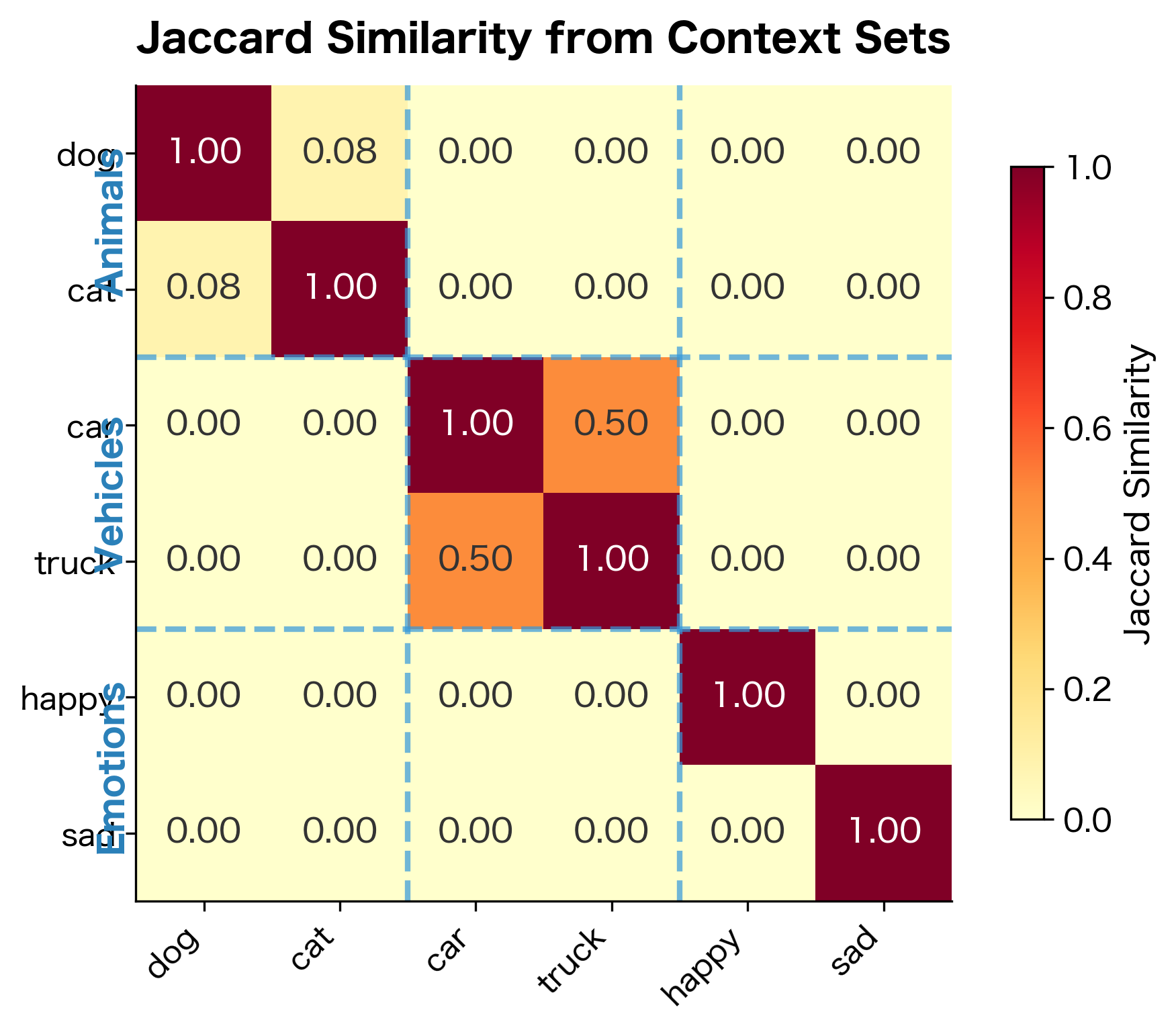
The result ranges from 0 (no overlap) to 1 (identical sets). If "dog" and "cat" both appear near the word "pet," that shared context contributes to their similarity.

In[7]:
Code
# Simple demonstration of distributional similarity
# Each word is represented by what words appear near it

word_contexts = {
    "dog": {"bark", "leash", "pet", "walk", "fetch", "loyal", "puppy"},
    "cat": {"meow", "purr", "pet", "scratch", "whiskers", "kitten"},
    "car": {"drive", "engine", "wheel", "road", "park", "gas"},
    "truck": {"drive", "engine", "wheel", "road", "haul", "cargo"},
    "happy": {"smile", "joy", "cheerful", "pleased", "content"},
    "sad": {"cry", "tears", "unhappy", "depressed", "gloomy"},
}


def jaccard_similarity(set1, set2):
    """
    Compute Jaccard similarity between two sets.

    Jaccard similarity measures the overlap between two sets:
    J(A, B) = |A ∩ B| / |A ∪ B|
    """
    intersection = len(set1 & set2)
    union = len(set1 | set2)
    return intersection / union if union > 0 else 0


# Compute pairwise similarities
words = list(word_contexts.keys())
similarities = {}
for i, w1 in enumerate(words):
    for w2 in words[i + 1 :]:
        sim = jaccard_similarity(word_contexts[w1], word_contexts[w2])
        similarities[(w1, w2)] = sim
Out[8]:
Console
Distributional Similarity (Jaccard on context sets):
--------------------------------------------------
  car    - truck : 0.50  shared: drive, engine, road, wheel
  dog    - cat   : 0.08  shared: pet
  dog    - car   : 0.00  shared: (none)
  dog    - truck : 0.00  shared: (none)
  dog    - happy : 0.00  shared: (none)
  dog    - sad   : 0.00  shared: (none)
  cat    - car   : 0.00  shared: (none)
  cat    - truck : 0.00  shared: (none)
  cat    - happy : 0.00  shared: (none)
  cat    - sad   : 0.00  shared: (none)
  car    - happy : 0.00  shared: (none)
  car    - sad   : 0.00  shared: (none)
  truck  - happy : 0.00  shared: (none)
  truck  - sad   : 0.00  shared: (none)
  happy  - sad   : 0.00  shared: (none)

The similarity scores align with our intuitions. "Dog" and "cat" share contexts (both are pets), as do "car" and "truck" (both are vehicles). Words from different semantic categories share few contexts and have low similarity.

Out[9]:
Visualization
Heatmap showing pairwise Jaccard similarities between six words, with clear clusters for animals, vehicles, and emotions.
Jaccard similarity matrix for words based on their context sets. The matrix reveals semantic clusters: animals (dog, cat) show moderate similarity, vehicles (car, truck) form another cluster, and emotions (happy, sad) cluster together despite being antonyms. Cross-category similarities are near zero, demonstrating how distributional patterns capture semantic categories.

Context Windows: Defining "Company"

What exactly counts as "context"? The distributional hypothesis requires us to define what it means for words to "appear together." The most common approach uses a context window: a fixed number of words before and after the target word.

Context Window

A context window defines the span of text around a target word that counts as its context. A window of size kk includes the kk words before and kk words after the target, capturing local co-occurrence patterns.

In[10]:
Code
def extract_contexts(text, target_word, window_size=2):
    """Extract context words within a window around the target word."""
    words = text.lower().split()
    contexts = []

    for i, word in enumerate(words):
        if word == target_word.lower():
            # Get words within window
            start = max(0, i - window_size)
            end = min(len(words), i + window_size + 1)

            context = []
            for j in range(start, end):
                if j != i:  # Exclude the target word itself
                    context.append(words[j])
            contexts.append(context)

    return contexts


# Example text
text = """The dog chased the cat across the yard. The cat climbed the tree. 
The dog barked at the cat. A friendly dog wagged its tail."""

# Extract contexts for "dog" with different window sizes
contexts_w1 = extract_contexts(text, "dog", window_size=1)
contexts_w2 = extract_contexts(text, "dog", window_size=2)
contexts_w3 = extract_contexts(text, "dog", window_size=3)
Out[11]:
Console
Context extraction for 'dog':
--------------------------------------------------

Window size = 1 (immediate neighbors):
  Occurrence 1: ['the', 'chased']
  Occurrence 2: ['the', 'barked']
  Occurrence 3: ['friendly', 'wagged']

Window size = 2:
  Occurrence 1: ['the', 'chased', 'the']
  Occurrence 2: ['tree.', 'the', 'barked', 'at']
  Occurrence 3: ['a', 'friendly', 'wagged', 'its']

Window size = 3:
  Occurrence 1: ['the', 'chased', 'the', 'cat']
  Occurrence 2: ['the', 'tree.', 'the', 'barked', 'at', 'the']
  Occurrence 3: ['cat.', 'a', 'friendly', 'wagged', 'its', 'tail.']

Window Size Effects

The choice of window size significantly affects what relationships we capture:

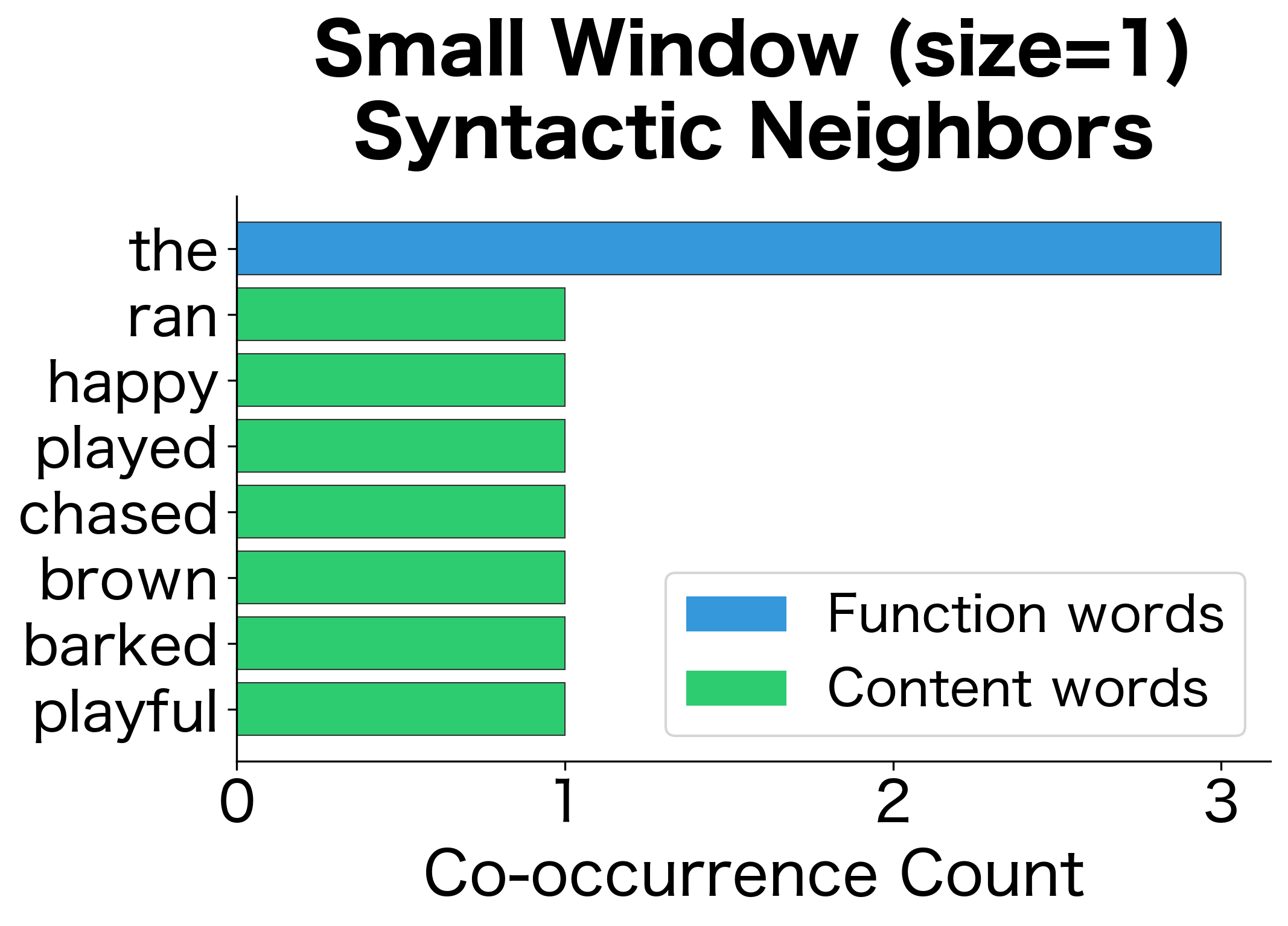
  • Small windows (1-2 words): Capture syntactic relationships and functional similarity. Words that share small-window contexts tend to be syntactically interchangeable.
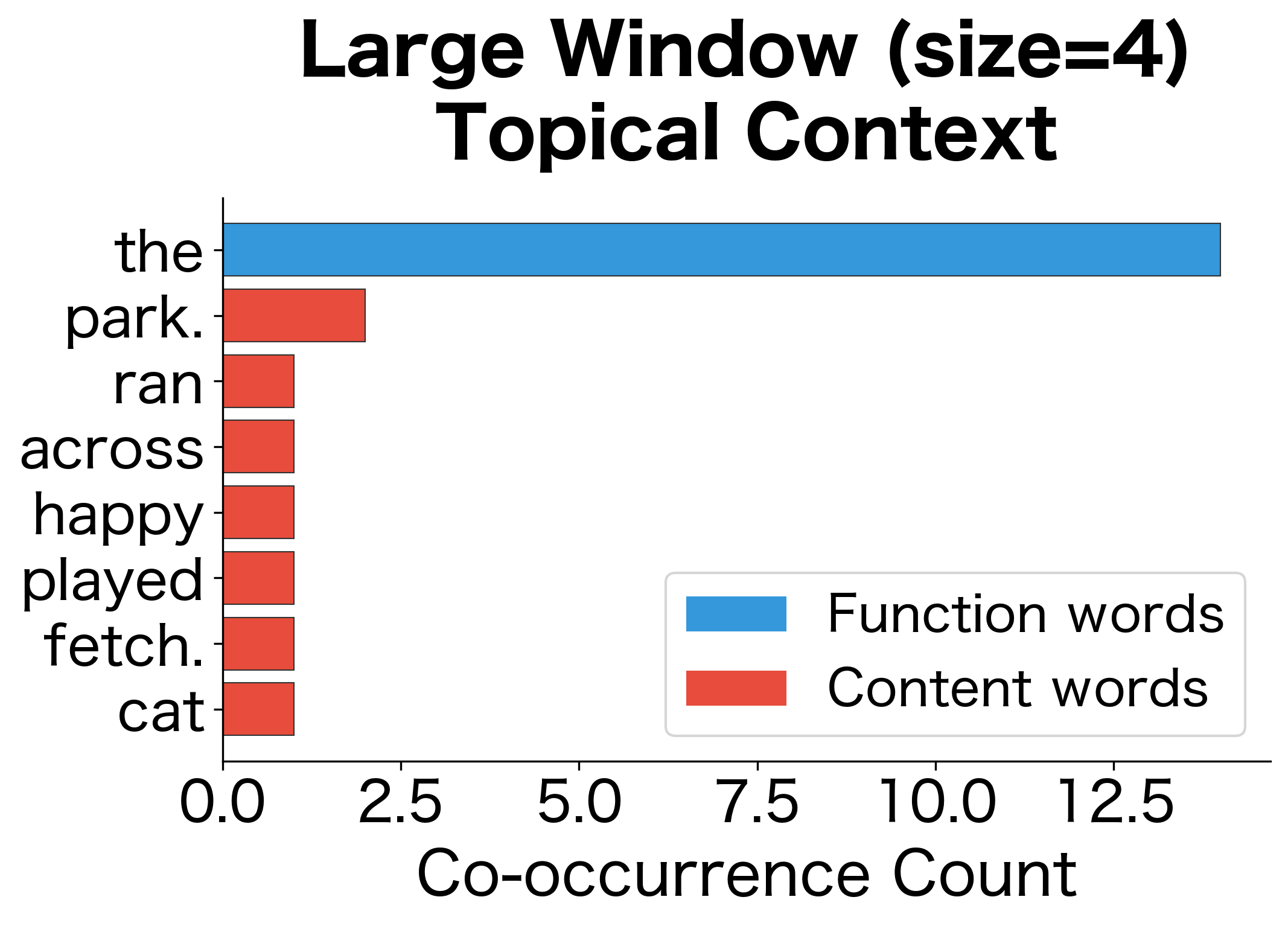
  • Large windows (5-10 words): Capture topical and semantic relationships. Words that share large-window contexts tend to appear in the same topics or domains.
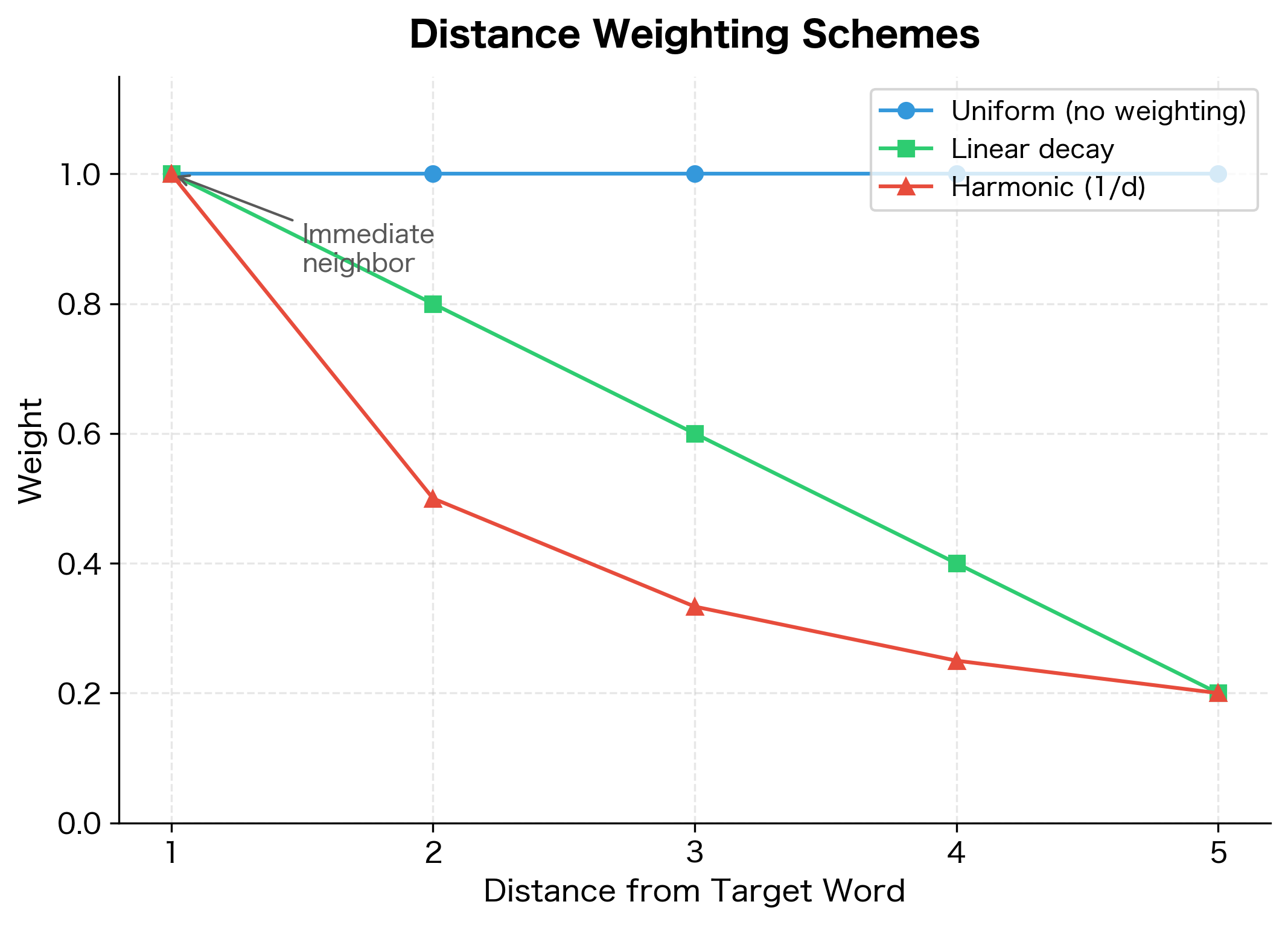
In[12]:
Code
from collections import Counter

# Larger corpus for more meaningful statistics
corpus = """
The dog ran across the park. The happy dog played fetch.
The cat sat on the mat. The lazy cat slept all day.
The dog chased the cat. The cat hissed at the dog.
A brown dog barked loudly. The small cat meowed softly.
The playful dog jumped high. The curious cat explored.
Dogs are loyal pets. Cats are independent animals.
The dog wagged its tail. The cat licked its paw.
"""


def build_context_vectors(corpus, window_size=2):
    """Build context frequency vectors for each word."""
    words = corpus.lower().split()
    word_contexts = {}

    for i, word in enumerate(words):
        if word not in word_contexts:
            word_contexts[word] = Counter()

        # Get context words
        start = max(0, i - window_size)
        end = min(len(words), i + window_size + 1)

        for j in range(start, end):
            if j != i:
                word_contexts[word][words[j]] += 1

    return word_contexts


# Build vectors with different window sizes
vectors_small = build_context_vectors(corpus, window_size=1)
vectors_large = build_context_vectors(corpus, window_size=4)
Out[13]:
Console
Top contexts for 'dog' and 'cat':
============================================================

Small window (size=1) - captures immediate neighbors:
  dog: [('the', 3), ('ran', 1), ('happy', 1), ('played', 1), ('chased', 1)]
  cat: [('the', 3), ('sat', 1), ('lazy', 1), ('slept', 1), ('hissed', 1)]

Large window (size=4) - captures broader context:
  dog: [('the', 14), ('park.', 2), ('ran', 1), ('across', 1), ('happy', 1)]
  cat: [('the', 12), ('mat.', 2), ('its', 2), ('dog', 1), ('played', 1)]
Out[14]:
Visualization
Two bar charts comparing context word frequencies for 'dog' with small and large window sizes.
Small window (size=1) captures immediate syntactic neighbors. Function words like 'the' dominate because they appear directly adjacent to content words.
Large window (size=4) captures broader topical context. More content words appear because the window extends across phrase boundaries.

Distance Weighting

Not all context words are equally informative. Words immediately adjacent to the target are more strongly associated than words several positions away. Many distributional models weight context words by their distance from the target.

In[15]:
Code
def build_weighted_context_vectors(corpus, window_size=3, weighting="linear"):
    """Build context vectors with distance-based weighting."""
    words = corpus.lower().split()
    word_contexts = {}

    for i, word in enumerate(words):
        if word not in word_contexts:
            word_contexts[word] = Counter()

        for j in range(
            max(0, i - window_size), min(len(words), i + window_size + 1)
        ):
            if j != i:
                distance = abs(j - i)

                if weighting == "linear":
                    # Weight decreases linearly with distance
                    weight = (window_size + 1 - distance) / window_size
                elif weighting == "harmonic":
                    # Weight is 1/distance
                    weight = 1 / distance
                else:
                    weight = 1  # No weighting

                word_contexts[word][words[j]] += weight

    return word_contexts


# Compare weighting schemes
vectors_unweighted = build_weighted_context_vectors(
    corpus, window_size=3, weighting="none"
)
vectors_linear = build_weighted_context_vectors(
    corpus, window_size=3, weighting="linear"
)
vectors_harmonic = build_weighted_context_vectors(
    corpus, window_size=3, weighting="harmonic"
)
Out[16]:
Console
Weighting schemes for 'dog' contexts (window=3):
-------------------------------------------------------

No weighting (all positions equal):
  the         : 10.00
  ran         : 1.00
  across      : 1.00
  park.       : 1.00
  happy       : 1.00

Linear weighting (closer = higher weight):
  the         : 6.33
  ran         : 1.00
  happy       : 1.00
  played      : 1.00
  chased      : 1.00

Harmonic weighting (weight = 1/distance):
  the         : 5.83
  ran         : 1.00
  happy       : 1.00
  played      : 1.00
  chased      : 1.00

Distance weighting emphasizes immediate neighbors while still capturing broader context. This often improves the quality of learned representations.

Out[17]:
Visualization
Line plot comparing three weighting schemes across distances 1-5, showing uniform as flat, linear as gradual decay, and harmonic as steep decay.
Comparison of distance weighting schemes. The plot shows how weight assigned to context words decreases with distance from the target word. Uniform weighting treats all positions equally, linear weighting provides gradual decay, and harmonic weighting (1/distance) strongly emphasizes immediate neighbors. The choice of weighting scheme affects which contextual relationships dominate the learned representations.

From Contexts to Vectors

We've established that words appearing in similar contexts have similar meanings. But how do we make this intuition computational? The key insight is that we can represent each word's "contextual profile" as a numerical vector, transforming the abstract notion of meaning into something we can measure and compare.

Think of it this way: if you wanted to describe a word's meaning through its usage patterns, you might list all the words that appear near it and how often. "Dog" appears near "bark" 5 times, near "walk" 3 times, near "cat" 2 times, and so on. This list of co-occurrence counts forms a fingerprint of the word's meaning. Two words with similar fingerprints likely have similar meanings.

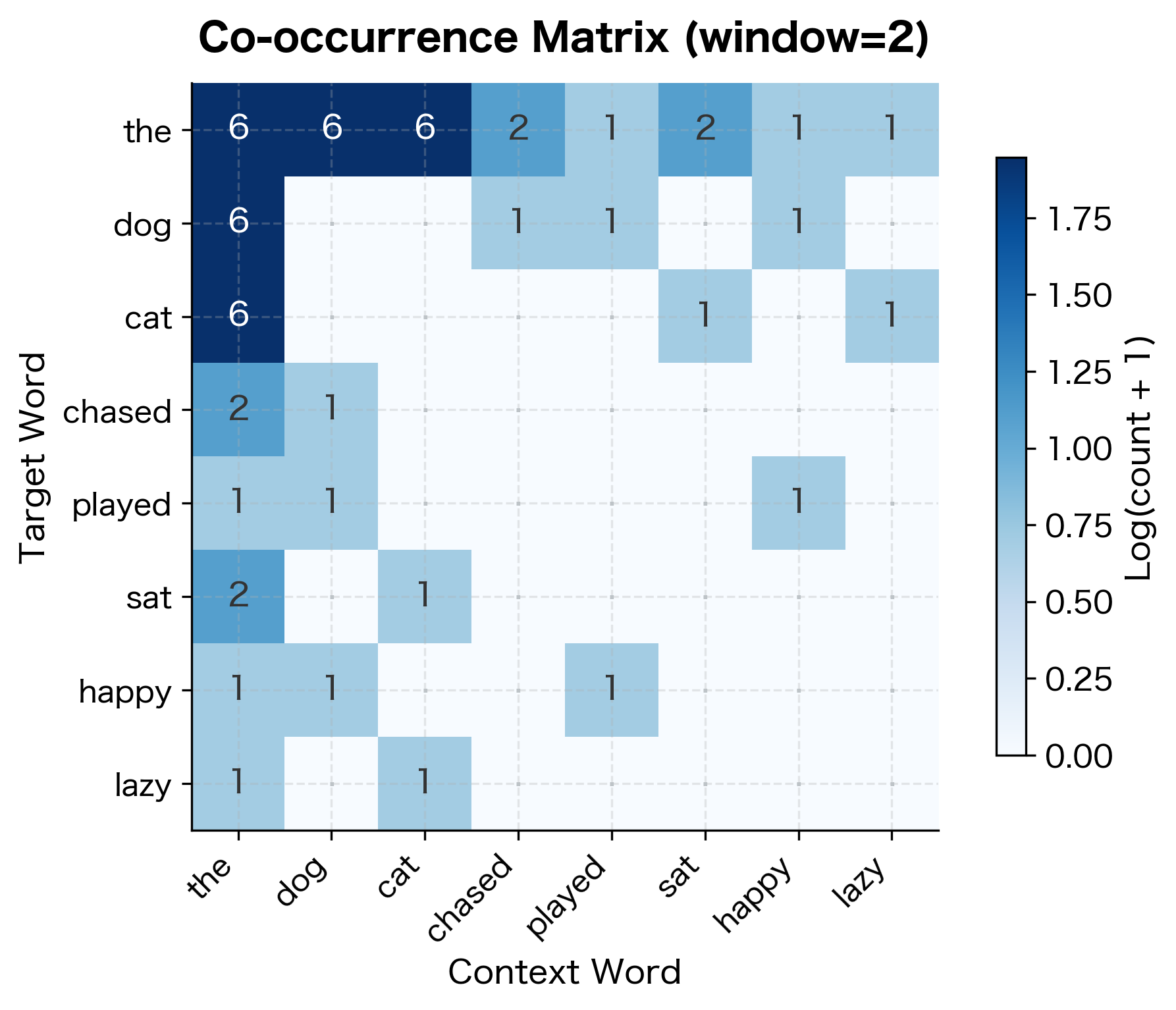
The Co-occurrence Matrix: Capturing Context Numerically

To formalize this intuition, we construct a co-occurrence matrix. This matrix has one row for each word in our vocabulary and one column for each possible context word (which is also the vocabulary). The entry at row ii, column jj counts how often word ii appears near word jj within our chosen context window.

The construction process works as follows:

  1. Build the vocabulary: Extract all unique words from the corpus that meet a minimum frequency threshold
  2. Initialize the matrix: Create a V×VV \times V matrix of zeros, where VV is the vocabulary size
  3. Scan the corpus: For each word, look at its context window and increment the corresponding matrix entries
  4. Result: Each row becomes a distributional vector representing that word's contextual associations
In[18]:
Code
import numpy as np
from collections import Counter


def build_cooccurrence_matrix(corpus, window_size=2, min_count=1):
    """Build a word-word co-occurrence matrix from corpus."""
    # Tokenize
    words = corpus.lower().split()

    # Build vocabulary
    word_counts = Counter(words)
    vocab = [w for w, c in word_counts.items() if c >= min_count]
    vocab = sorted(vocab)
    word_to_idx = {w: i for i, w in enumerate(vocab)}

    # Build co-occurrence matrix
    n = len(vocab)
    matrix = np.zeros((n, n))

    for i, word in enumerate(words):
        if word not in word_to_idx:
            continue
        word_idx = word_to_idx[word]

        # Count co-occurrences within window
        for j in range(
            max(0, i - window_size), min(len(words), i + window_size + 1)
        ):
            if j != i and words[j] in word_to_idx:
                context_idx = word_to_idx[words[j]]
                matrix[word_idx, context_idx] += 1

    return matrix, vocab, word_to_idx


# Build matrix from our corpus
matrix, vocab, word_to_idx = build_cooccurrence_matrix(corpus, window_size=2)
Out[19]:
Console
Co-occurrence matrix shape: (45, 45)
Vocabulary size: 45

Sample vocabulary words:
  ['a', 'across', 'all', 'animals.', 'are', 'at', 'barked', 'brown', 'cat', 'cat.']

Distributional vectors (first 10 dimensions):
  dog: [1. 1. 0. 1. 0. 0. 1. 1. 0. 0.]
  cat: [0. 0. 1. 0. 0. 1. 0. 0. 0. 1.]

Each row of this matrix is now a distributional vector for a word. The vector captures how often that word co-occurs with every other word in the vocabulary. Words with similar vectors should have similar meanings, but how do we measure "similar"?

Out[20]:
Visualization
Heatmap of co-occurrence counts between selected words, showing symmetric patterns with function words having high counts across the board.
Visualization of a co-occurrence matrix for selected words. Each cell shows how often the row word appears near the column word. The matrix is symmetric (if 'dog' appears near 'cat', then 'cat' appears near 'dog'). Notice how 'the' co-occurs with everything (it's a function word), while content words like 'dog' and 'cat' have more selective patterns.

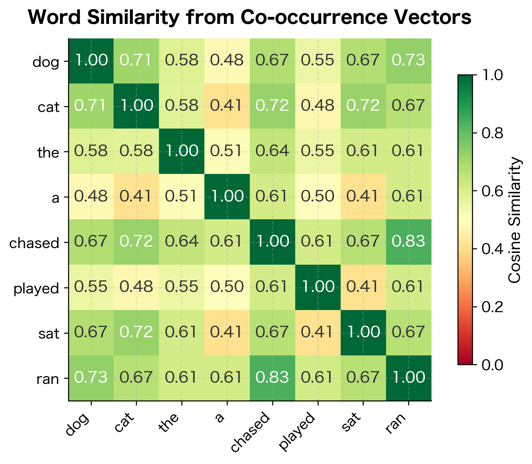
Computing Word Similarity: From Vectors to Meaning

With words represented as vectors in a high-dimensional space, we need a way to measure how "close" two vectors are. The most intuitive approach might be Euclidean distance, but this has a problem: it's sensitive to vector magnitude. A word that appears 1,000 times will have much larger co-occurrence counts than a word appearing 10 times, even if their contextual patterns are identical.

Cosine similarity solves this by measuring the angle between vectors rather than their distance. Two vectors pointing in the same direction have cosine similarity of 1, regardless of their lengths. Perpendicular vectors have similarity 0, and opposite vectors have similarity -1.

The formula captures this geometric intuition:

cosine(u,v)=uvuv\text{cosine}(\vec{u}, \vec{v}) = \frac{\vec{u} \cdot \vec{v}}{\|\vec{u}\| \cdot \|\vec{v}\|}

where:

  • u,v\vec{u}, \vec{v}: the two word vectors being compared
  • uv\vec{u} \cdot \vec{v}: the dot product of the two vectors
  • u,v\|\vec{u}\|, \|\vec{v}\|: the magnitudes (lengths) of the vectors

Let's unpack what each component means:

  • The numerator uv=iuivi\vec{u} \cdot \vec{v} = \sum_i u_i v_i is the dot product. It sums the products of corresponding components. When both vectors have high values in the same dimensions (they co-occur with the same words), the dot product is large.

  • The denominator uv\|\vec{u}\| \cdot \|\vec{v}\| normalizes by vector magnitudes. The magnitude u=iui2\|\vec{u}\| = \sqrt{\sum_i u_i^2} measures the overall "size" of the vector. Dividing by magnitudes ensures that frequent and rare words can be compared fairly.

Expanding the formula completely with all terms written out:

cosine(u,v)=iuiviiui2ivi2\text{cosine}(\vec{u}, \vec{v}) = \frac{\sum_i u_i v_i}{\sqrt{\sum_i u_i^2} \cdot \sqrt{\sum_i v_i^2}}

where:

  • uiu_i: the ii-th component of vector u\vec{u} (co-occurrence count of the first word with the ii-th vocabulary word)
  • viv_i: the ii-th component of vector v\vec{v} (co-occurrence count of the second word with the ii-th vocabulary word)
  • iuivi\sum_i u_i v_i: the sum over all dimensions, computing element-wise products
  • iui2\sqrt{\sum_i u_i^2}: the Euclidean norm of u\vec{u}
  • ivi2\sqrt{\sum_i v_i^2}: the Euclidean norm of v\vec{v}

The result ranges from -1 (vectors pointing in opposite directions) to 1 (vectors pointing in the same direction). For co-occurrence vectors, which have only non-negative entries, cosine similarity ranges from 0 to 1.

In[21]:
Code
def cosine_similarity(vec1, vec2):
    """Compute cosine similarity between two vectors."""
    dot_product = np.dot(vec1, vec2)
    norm1 = np.linalg.norm(vec1)
    norm2 = np.linalg.norm(vec2)

    if norm1 == 0 or norm2 == 0:
        return 0.0

    return dot_product / (norm1 * norm2)


def find_most_similar(word, matrix, vocab, word_to_idx, top_n=5):
    """Find the most similar words to a target word."""
    if word not in word_to_idx:
        return []

    word_idx = word_to_idx[word]
    word_vec = matrix[word_idx]

    similarities = []
    for other_word, other_idx in word_to_idx.items():
        if other_word != word:
            sim = cosine_similarity(word_vec, matrix[other_idx])
            similarities.append((other_word, sim))

    return sorted(similarities, key=lambda x: x[1], reverse=True)[:top_n]


# Find similar words
similar_to_dog = find_most_similar("dog", matrix, vocab, word_to_idx)
similar_to_cat = find_most_similar("cat", matrix, vocab, word_to_idx)
Out[22]:
Console
Most similar words (by distributional similarity):
---------------------------------------------

Similar to 'dog':
  park.          : 0.785
  cat.           : 0.729
  ran            : 0.729
  cat            : 0.710
  chased         : 0.673

Similar to 'cat':
  mat.           : 0.778
  chased         : 0.722
  hissed         : 0.722
  sat            : 0.722
  dog            : 0.710

The results demonstrate the distributional hypothesis in action. Words appearing in similar contexts (sharing high co-occurrence with the same vocabulary items) receive high cosine similarity scores. The mathematical machinery transforms our linguistic intuition into a computable quantity.

Out[23]:
Visualization
Heatmap showing pairwise cosine similarities between words, with darker colors for higher similarity.
Cosine similarity matrix for selected words from our corpus. Warmer colors indicate higher similarity. Notice that 'dog' and 'cat' show moderate similarity (both are animals), while function words like 'the' form their own cluster. The symmetric matrix reflects the symmetric nature of co-occurrence.

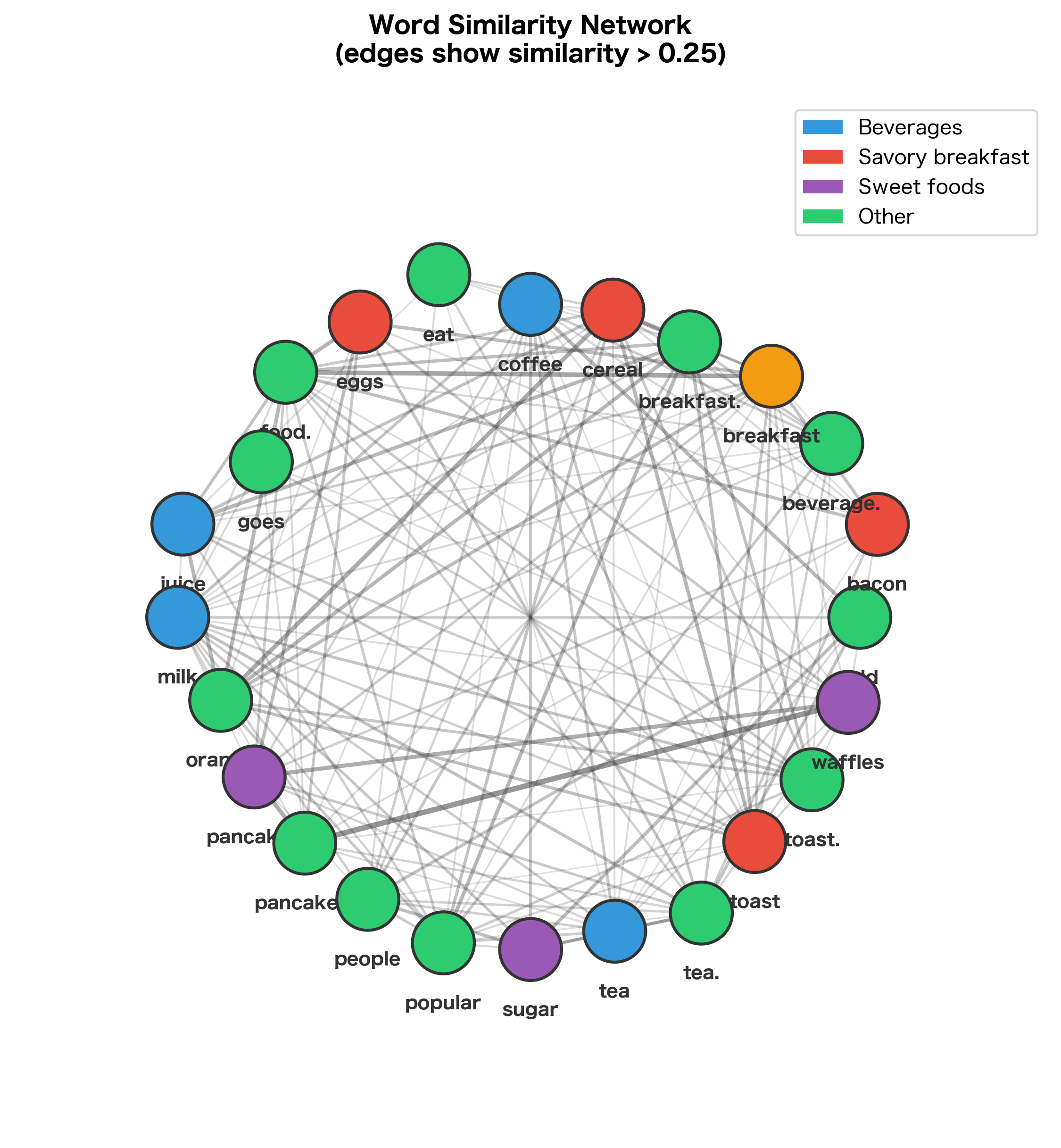
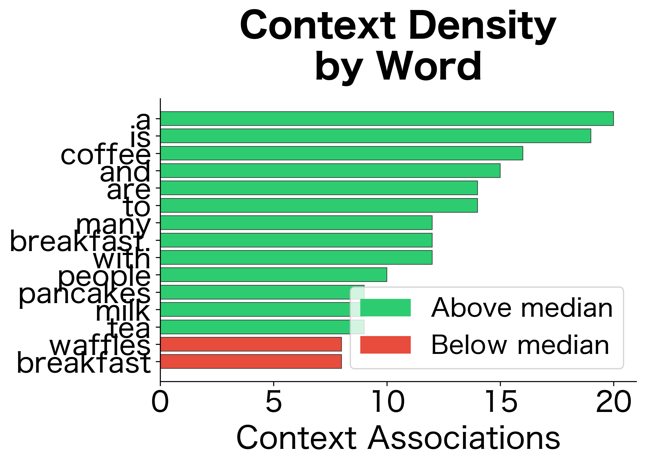
A Worked Example: Discovering Word Relationships

Let's work through a complete example using a larger corpus to see the distributional hypothesis in action.

In[24]:
Code
# A more substantial corpus about food and cooking
food_corpus = """
Coffee is a popular morning beverage. Many people drink coffee with breakfast.
Tea is another popular beverage. Some prefer tea to coffee.
Both coffee and tea contain caffeine. Caffeine helps people wake up.
Bread is a staple food. Toast is made from bread. People eat toast for breakfast.
Butter goes well on toast. Jam is also spread on toast.
Milk is a dairy product. People add milk to coffee and tea.
Sugar sweetens beverages. Many add sugar to their coffee or tea.
Eggs are a breakfast food. Scrambled eggs are popular. Fried eggs are tasty.
Bacon is often served with eggs. Bacon and eggs make a classic breakfast.
Orange juice is a breakfast drink. Fresh orange juice is healthy.
Cereal is a quick breakfast. Many eat cereal with milk.
Pancakes are a weekend breakfast treat. Syrup goes on pancakes.
Waffles are similar to pancakes. Both pancakes and waffles are sweet.
"""

# Build co-occurrence matrix with larger window
food_matrix, food_vocab, food_word_to_idx = build_cooccurrence_matrix(
    food_corpus, window_size=3, min_count=2
)
Out[25]:
Console
Food corpus statistics:
  Vocabulary size: 33
  Matrix shape: (33, 33)

Distributional similarities:
--------------------------------------------------

'coffee':
    add         : 0.611
    both        : 0.583
    many        : 0.559
    and         : 0.546

'tea':
    and         : 0.563
    to          : 0.537
    tea.        : 0.490
    coffee      : 0.473

'breakfast':
    food.       : 0.771
    is          : 0.585
    orange      : 0.570
    eggs        : 0.565

'eggs':
    food.       : 0.639
    breakfast   : 0.565
    pancakes    : 0.561
    tea.        : 0.503

The distributional analysis correctly identifies that "coffee" and "tea" are similar (both are beverages), and that "breakfast" is associated with food items. These relationships emerged purely from co-occurrence patterns, not from any predefined knowledge.

Out[26]:
Visualization
Network graph showing word relationships with edges between similar words and clusters for beverages, breakfast foods, and sweets.
Word similarity network derived from the food corpus. Edges connect words with cosine similarity above 0.3. Clusters emerge naturally: beverages (coffee, tea, milk), breakfast foods (eggs, bacon, toast), and sweet items (pancakes, waffles, syrup). The network structure reflects semantic relationships learned purely from co-occurrence patterns.

Limitations of Distributional Semantics

The distributional hypothesis works well in many cases, but it has limitations. Understanding these limitations helps explain why more sophisticated approaches like neural word embeddings were developed.

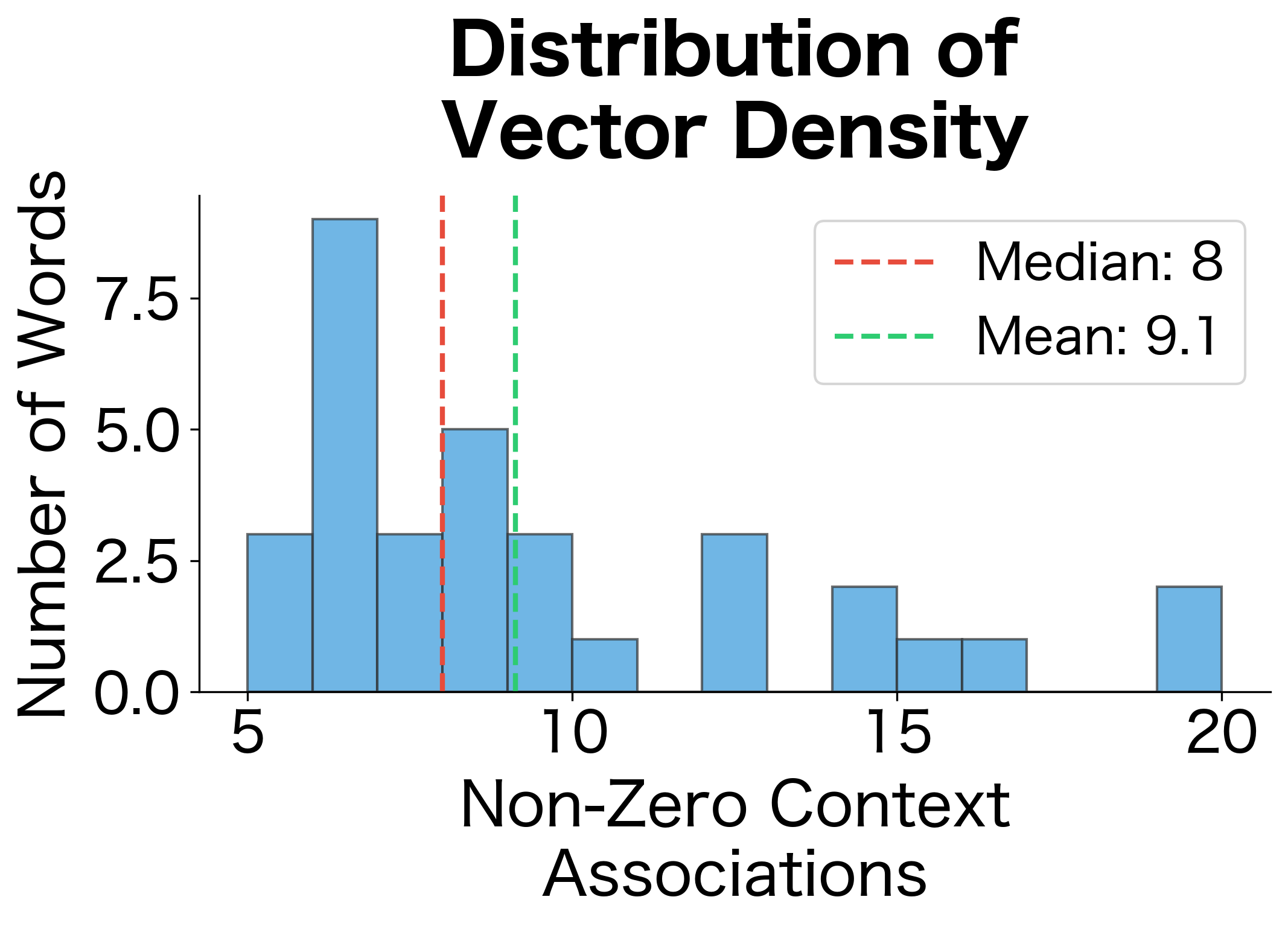
The Sparsity Problem

Co-occurrence matrices are extremely sparse. Most word pairs never appear together, even in large corpora. This sparsity makes similarity estimates unreliable for rare words.

In[27]:
Code
# Analyze sparsity of our co-occurrence matrix
total_entries = food_matrix.size
nonzero_entries = np.count_nonzero(food_matrix)
sparsity = 1 - (nonzero_entries / total_entries)

# Count how many words have very sparse vectors
words_with_few_contexts = sum(
    1 for i in range(len(food_vocab)) if np.count_nonzero(food_matrix[i]) < 5
)
Out[28]:
Console
Sparsity Analysis:
---------------------------------------------
Matrix size:        33 × 33
Total entries:      1,089
Non-zero entries:   301
Sparsity:           72.4%

Words with < 5 context words: 0 of 33

This high sparsity level reveals a fundamental challenge: most word pairs in the vocabulary never co-occur, leaving the majority of matrix entries at zero. Words with fewer than 5 context associations have vectors so sparse that similarity calculations become unreliable. This sparsity problem motivates dimensionality reduction techniques that we'll explore in later chapters.

Out[29]:
Visualization
Histogram and bar chart showing the distribution of non-zero entries per word in the co-occurrence matrix.
Distribution of vector density across words. Most words have few context associations, with median and mean shown by dashed lines.
Context density by word, sorted by number of associations. Words above median (green) have more reliable vectors than those below (red).

Polysemy and Homonymy

The distributional hypothesis treats each word form as a single unit, but words can have multiple meanings. The word "bank" (financial institution vs. river bank) gets a single vector that mixes both meanings together.

In[30]:
Code
# Demonstrating the polysemy problem
polysemy_corpus = """
I deposited money at the bank. The bank approved my loan.
We sat by the river bank. The bank of the river was muddy.
The bank teller was helpful. Fish swam near the bank.
My bank account has low fees. The steep bank led to water.
"""

# Both meanings of "bank" get mixed together
polysemy_matrix, polysemy_vocab, polysemy_idx = build_cooccurrence_matrix(
    polysemy_corpus, window_size=2
)

bank_idx = polysemy_idx.get("bank", -1)
bank_contexts = {}
if bank_idx >= 0:
    for i, word in enumerate(polysemy_vocab):
        if polysemy_matrix[bank_idx, i] > 0:
            bank_contexts[word] = polysemy_matrix[bank_idx, i]
Out[31]:
Console
Polysemy problem: 'bank' has multiple meanings
--------------------------------------------------

Contexts for 'bank' (mixed meanings):

  Financial contexts:
    approved: 1
    teller: 1
    account: 1

  Nature contexts:
    steep: 1

The single "bank" vector conflates contexts from two completely different meanings: financial institutions and river edges. When computing similarity, this mixed vector will show partial similarity to both "money" and "river," potentially misleading downstream applications. Contextual embeddings like BERT address this by generating different vectors for "bank" depending on the surrounding sentence.

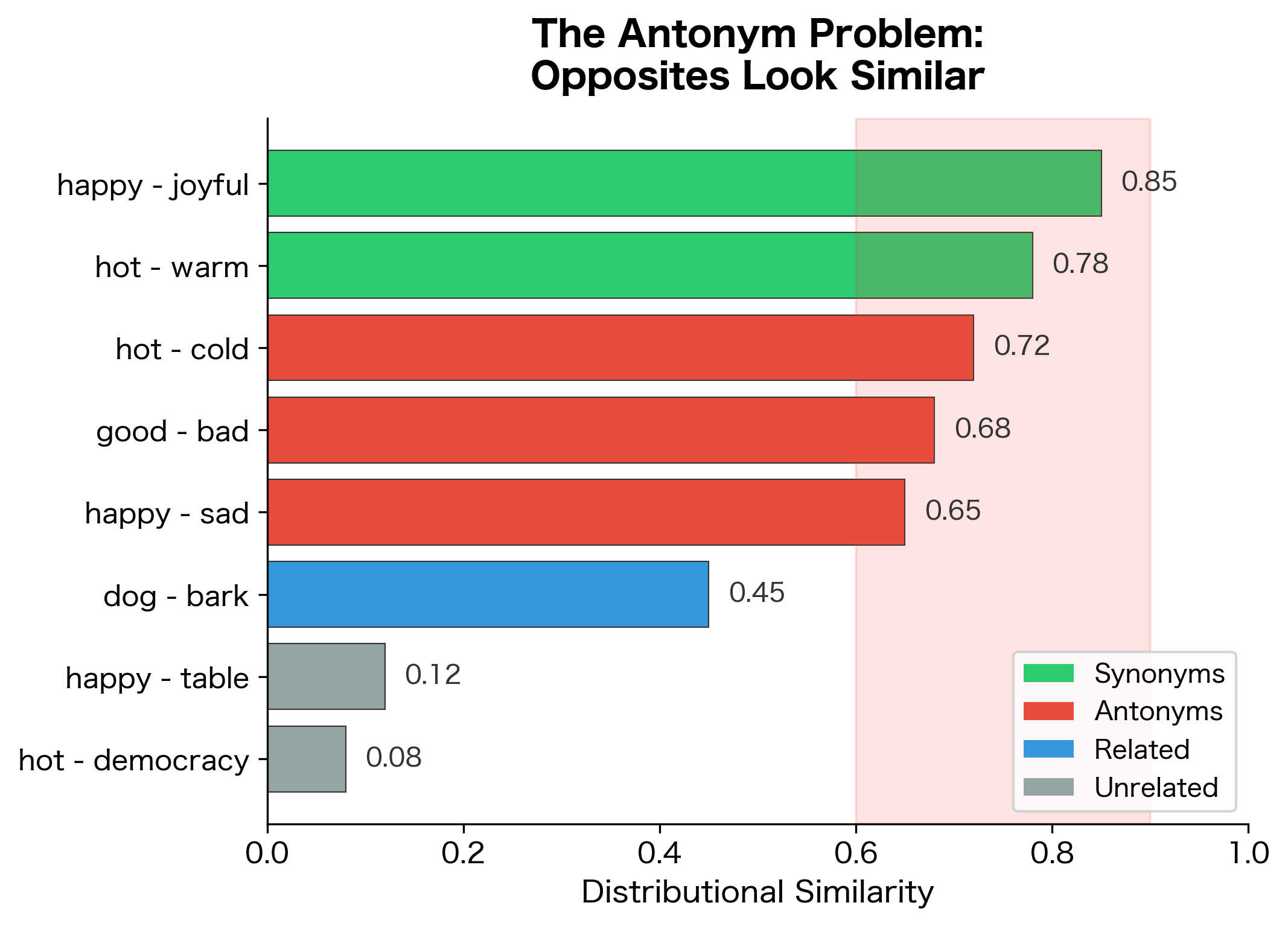
Antonyms Have Similar Distributions

Here's a surprising limitation: antonyms often appear in similar contexts. "Hot" and "cold," "good" and "bad," "happy" and "sad" can substitute for each other in many sentences. Distributional semantics struggles to distinguish opposites from synonyms.

In[32]:
Code
# Antonyms in similar contexts
antonym_examples = [
    ("The weather is ___", ["hot", "cold"]),
    ("The movie was ___", ["good", "bad"]),
    ("She felt very ___", ["happy", "sad"]),
    ("The test was ___", ["easy", "hard"]),
]

# Both members of each pair fit the same contexts
Out[33]:
Console
Antonym problem: opposites share contexts
--------------------------------------------------

'The weather is ___'
  Both fit: hot and cold

'The movie was ___'
  Both fit: good and bad

'She felt very ___'
  Both fit: happy and sad

'The test was ___'
  Both fit: easy and hard

Each template accepts both members of an antonym pair because they share grammatical properties (both are adjectives, both describe the same kind of entity). Distributional semantics captures this syntactic interchangeability but cannot distinguish that the words have opposite meanings. This limitation shows why purely distributional approaches sometimes need supplementary knowledge sources to capture semantic relations like antonymy.

Out[34]:
Visualization
Bar chart comparing similarity scores for synonym pairs, antonym pairs, and unrelated pairs, showing that antonyms have unexpectedly high similarity.
The antonym problem in distributional semantics. Synonyms (happy-joyful) correctly show high similarity, but antonyms (hot-cold, good-bad) also show high similarity because they appear in the same syntactic contexts. The red shaded region highlights how distributional methods struggle to distinguish 'similar meaning' from 'opposite meaning'.

Compositionality

Word meaning often depends on combination. "Hot dog" doesn't mean a warm canine. "Kick the bucket" doesn't involve feet or pails. Distributional semantics at the word level cannot capture these compositional meanings.
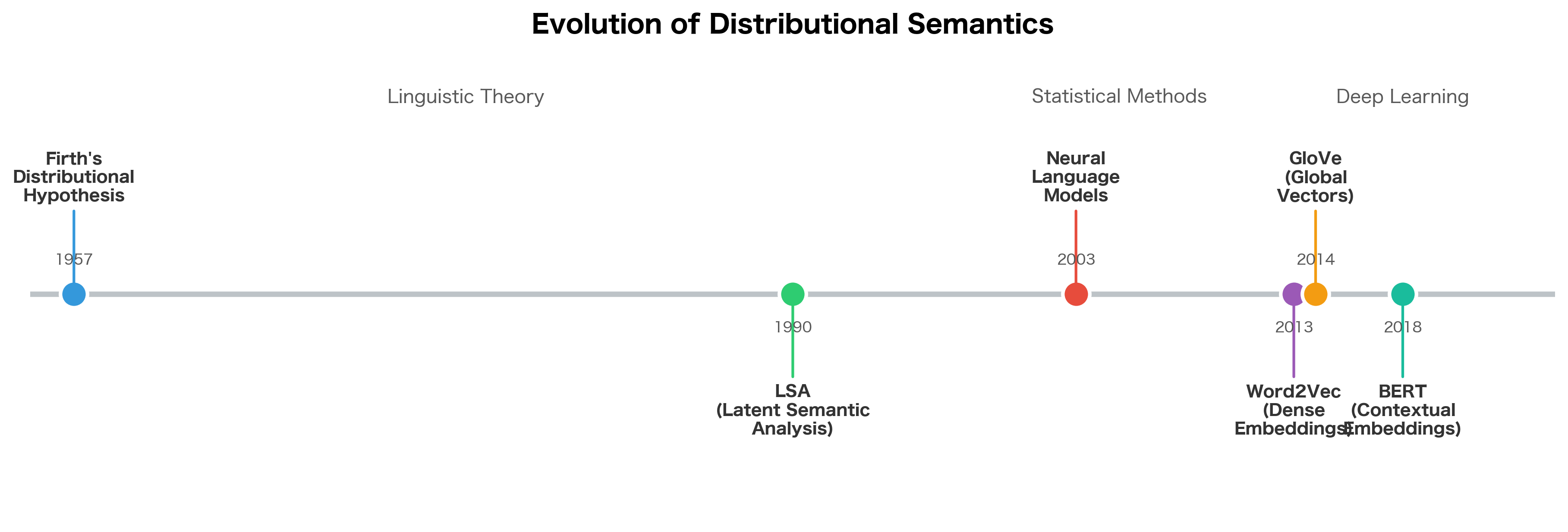
Impact on NLP

Despite its limitations, the distributional hypothesis shaped computational linguistics and laid the groundwork for modern NLP:

  • Vector space models: The idea that meaning can be represented as points in a high-dimensional space, where distance reflects similarity, remains central to NLP. Modern word embeddings (Word2Vec, GloVe) are direct descendants of distributional semantics.
  • Unsupervised learning: Distributional methods learn from raw text without labeled examples. This self-supervised approach, learning structure from data itself, set the stage for pretraining in deep learning.
  • Similarity as a primitive: Measuring word similarity enables many applications: information retrieval, question answering, machine translation, and more. The distributional hypothesis provides a clear way to compute similarity.
  • Contextual meaning: The insight that context determines meaning points toward contextual embeddings (ELMo, BERT) where the same word gets different representations based on its context.
Out[35]:
Visualization
Timeline showing progression from 1957 Firth to 2018 BERT with key milestones in distributional semantics.
Evolution of distributional semantics from Firth's 1957 insight to modern contextual embeddings. Each advance built on the core idea that meaning emerges from context. Early methods used sparse co-occurrence matrices, while modern approaches learn dense vectors through neural networks.

Key Parameters

When building distributional representations, several parameters significantly affect the quality and characteristics of the resulting word vectors:

window_size: The number of words on each side of the target to include as context.

  • Small values (1-2): Capture syntactic relationships and functional similarity. Words that share small-window contexts tend to be syntactically interchangeable (e.g., "dog" and "cat" as nouns).
  • Large values (5-10): Capture topical and semantic relationships. Words that share large-window contexts tend to appear in the same domains (e.g., "doctor" and "hospital").
  • Typical starting point: 2-5 for most applications.

min_count: Minimum frequency threshold for including words in the vocabulary.

  • Low values (1-2): Include rare words, but their vectors may be unreliable due to sparse data.
  • Higher values (5-10): More reliable vectors for included words, but rare words are excluded.
  • Trade-off: Vocabulary coverage vs. vector quality.

weighting: How to weight context words based on distance from target.

  • 'none': All positions within window weighted equally (weight = 1 for all).
  • 'linear': Weight decreases linearly with distance. For a window of size kk, the weight at distance dd is (k+1d)/k(k + 1 - d) / k. Closer words contribute more.
  • 'harmonic': Weight is 1/d1/d where dd is the distance from the target word. Strong emphasis on immediate neighbors (distance 1 gets weight 1, distance 2 gets weight 0.5, etc.).
  • Recommendation: Linear or harmonic weighting typically improves vector quality.

Similarity metric: How to measure similarity between word vectors.

  • Cosine similarity: Most common choice. Measures angle between vectors, ignoring magnitude. Values range from -1 to 1, with 1 indicating identical direction.
  • Euclidean distance: Sensitive to vector magnitude. Less common for distributional vectors.
  • Jaccard similarity: For binary or set-based representations. Measures overlap between context sets.

Summary

The distributional hypothesis, that words appearing in similar contexts have similar meanings, provides a solid foundation for representing word meaning computationally. From Firth's linguistic insight to modern neural embeddings, this idea has shaped how we teach machines to understand language.

Key takeaways:

  • "You shall know a word by the company it keeps": Context reveals meaning, enabling unsupervised learning of semantic representations
  • Paradigmatic vs syntagmatic relations: Words can be similar by substitutability (paradigmatic) or by co-occurrence (syntagmatic)
  • Context windows define what counts as "company," with smaller windows capturing syntax and larger windows capturing topics
  • Distance weighting emphasizes immediate neighbors, improving representation quality
  • Vector representations enable mathematical operations on meaning, including similarity computation via cosine similarity
  • Limitations include sparsity, polysemy conflation, antonym confusion, and lack of compositionality

The next chapter builds directly on these foundations, showing how to construct and analyze co-occurrence matrices at scale, transforming the distributional hypothesis into a practical computational tool.

Quiz

Ready to test your understanding? Take this quick quiz to reinforce what you've learned about the distributional hypothesis and how context reveals word meaning.

Loading component...

Reference

BIBTEXAcademic
@misc{thedistributionalhypothesishowcontextrevealswordmeaning, author = {Michael Brenndoerfer}, title = {The Distributional Hypothesis: How Context Reveals Word Meaning}, year = {2025}, url = {https://mbrenndoerfer.com/writing/distributional-hypothesis-word-meaning-context}, organization = {mbrenndoerfer.com}, note = {Accessed: 2025-01-01} }
APAAcademic
Michael Brenndoerfer (2025). The Distributional Hypothesis: How Context Reveals Word Meaning. Retrieved from https://mbrenndoerfer.com/writing/distributional-hypothesis-word-meaning-context
MLAAcademic
Michael Brenndoerfer. "The Distributional Hypothesis: How Context Reveals Word Meaning." 2026. Web. today. <https://mbrenndoerfer.com/writing/distributional-hypothesis-word-meaning-context>.
CHICAGOAcademic
Michael Brenndoerfer. "The Distributional Hypothesis: How Context Reveals Word Meaning." Accessed today. https://mbrenndoerfer.com/writing/distributional-hypothesis-word-meaning-context.
HARVARDAcademic
Michael Brenndoerfer (2025) 'The Distributional Hypothesis: How Context Reveals Word Meaning'. Available at: https://mbrenndoerfer.com/writing/distributional-hypothesis-word-meaning-context (Accessed: today).
SimpleBasic
Michael Brenndoerfer (2025). The Distributional Hypothesis: How Context Reveals Word Meaning. https://mbrenndoerfer.com/writing/distributional-hypothesis-word-meaning-context