

Master the Vehicle Routing Problem with Time Windows (VRPTW), including mathematical formulation, constraint programming, and practical implementation using Google OR-Tools for logistics optimization.

This article is part of the free-to-read Machine Learning from Scratch
Choose your expertise level to adjust how many terms are explained. Beginners see more tooltips, experts see fewer to maintain reading flow. Hover over underlined terms for instant definitions.
Vehicle Routing Problem with Time Windows (VRPTW)
The Vehicle Routing Problem with Time Windows (VRPTW) is a fundamental optimization challenge in logistics and supply chain management. At its core, VRPTW seeks to determine the most efficient routes for a fleet of vehicles to serve a set of customers, where each customer must be visited within a specific time window. This problem extends the classic Vehicle Routing Problem (VRP) by incorporating temporal constraints that reflect real-world delivery scenarios where customers have preferred or required service times.
The VRPTW is particularly relevant in modern logistics operations, from e-commerce delivery to field service management. Unlike simple routing problems that only consider distance or travel time, VRPTW must balance multiple competing objectives: minimizing total travel cost, respecting vehicle capacity constraints, and ensuring all customers are served within their specified time windows. This makes it a complex combinatorial optimization problem that often requires sophisticated algorithms to solve efficiently.
The problem becomes exponentially more complex as the number of customers and vehicles increases, making it computationally challenging for large-scale instances. However, modern optimization tools like Google OR-Tools provide powerful solvers that can handle realistic problem sizes while finding high-quality solutions in reasonable time.
Advantages
VRPTW solutions can significantly reduce total travel time and distance, leading to lower fuel costs, reduced vehicle wear, and improved driver productivity. By optimizing routes, companies can serve more customers with the same fleet size or maintain service levels with fewer vehicles. These operational efficiencies translate directly to bottom-line savings, making VRPTW optimization a high-value investment for logistics operations of any scale.
Time window constraints ensure that deliveries arrive when customers expect them, improving service quality and customer satisfaction. This is particularly important for time-sensitive deliveries like medical supplies, perishable goods, or scheduled appointments where late arrivals can have serious consequences. By explicitly modeling customer preferences, VRPTW solutions help businesses build trust and maintain strong customer relationships.
Modern VRPTW solvers can handle problems with hundreds of customers and dozens of vehicles, making them suitable for real-world applications. The solutions can be updated dynamically as new orders arrive or conditions change, allowing dispatchers to respond to evolving circumstances throughout the day. This scalability and adaptability make VRPTW a practical tool for both strategic route planning and day-to-day operational decisions.
Disadvantages
As a variant of the Traveling Salesman Problem, VRPTW is NP-hard, meaning solution time grows exponentially with problem size. While modern solvers can handle realistic instances with hundreds of customers, very large problems may require heuristic approaches or problem decomposition strategies that sacrifice guaranteed optimality for computational tractability.
Finding optimal solutions for large instances can be computationally expensive, forcing practitioners to balance solution quality with computation time. In practice, this often means accepting near-optimal solutions that can be found quickly rather than waiting hours or days for provably optimal routes. The gap between the best-known solution and the theoretical optimum may be acceptable for operational purposes but can be frustrating when marginal improvements matter.
Real-world routing often involves dynamic changes such as new orders arriving throughout the day, unexpected traffic conditions, or vehicle breakdowns that can invalidate pre-computed solutions. This volatility requires either frequent re-optimization, which adds computational overhead, or robust solution approaches that build in slack to accommodate changes. Neither approach is perfect, and dispatchers must often make real-time adjustments that deviate from the optimized plan.
Formula
Every optimization problem tells a story of choices and consequences. In VRPTW, the story begins with a simple question: How do we teach a computer to make the same decisions a skilled dispatcher makes instinctively? A human dispatcher juggles multiple concerns simultaneously: which truck goes where, what time to arrive, how much each vehicle can carry. To solve this problem computationally, we must translate this intuition into precise mathematical language.
This section develops the mathematical formulation step by step. For each component, we'll ask: Why do we need this? and What happens if we leave it out? By the end, you'll understand both what the formulas say and why each component is important for capturing the real-world complexity of vehicle routing.
The Dispatcher's Dilemma: Three Intertwined Decisions
Picture yourself as a logistics dispatcher on a Monday morning. You have a fleet of delivery trucks, a list of customers expecting packages, and a day's worth of time windows to honor. Your job is to answer three fundamental questions:
- Assignment: Which vehicle should visit which customers?
- Sequencing: In what order should each vehicle make its stops?
- Timing: When exactly should each vehicle arrive at each location?
At first glance, these might seem like separate problems. But consider what happens when you try to solve them independently:
- You assign Customer A to Truck 1 because it's nearby, but Truck 1 is already overloaded.
- You sequence Customer B before Customer C because B is closer to the depot, but Customer B's time window doesn't open until the afternoon.
- You schedule an arrival at 10:00 AM, but given travel times, the truck can't possibly get there before noon.
The fundamental insight is that these three decisions are deeply interconnected. The sequence of visits determines travel times, which determine arrival times, which must fit within time windows, which constrain which sequences are feasible, which affects how we assign customers to vehicles. It's a web of dependencies that we must capture mathematically.
The Language of Optimization: Parameters and Variables
Before we can express our dispatcher's decisions mathematically, we need to establish a precise vocabulary. In optimization, we distinguish between two types of quantities:
- Parameters: Fixed information about the problem that we cannot change
- Decision variables: The unknowns that the solver must determine
Think of parameters as the rules of the game, and decision variables as the moves we're trying to optimize.
Throughout this formulation, we use the following notation:
| Symbol | Type | Meaning |
|---|---|---|
| Set | All locations (0 = depot, others = customers) | |
| Set | Available vehicles | |
| Set | Possible direct connections (arcs) | |
| Parameter | Demand at customer | |
| Parameter | Capacity of vehicle | |
| Parameter | Travel time from location to | |
| Parameter | Time window at location | |
| Parameter | Service time at location | |
| Parameter | Cost of traveling from to | |
| Decision variable | 1 if vehicle travels from to , 0 otherwise | |
| Decision variable | Arrival time of vehicle at location | |
| Constant | Large value for Big-M constraints |
The Problem Landscape (Parameters):
The world we're optimizing within is defined by several fixed quantities:
-
Locations (): The depot (node 0) serves as home base, where all vehicles start and must return. The remaining nodes represent customers awaiting service.
-
Fleet (): We have vehicles at our disposal. Each vehicle has a capacity representing the maximum total demand it can carry. A delivery van might hold 20 packages; a truck might have a 10-ton weight limit.
-
Network (): Between any two locations, there exists a potential route. The arc represents the possibility of traveling directly from to , with travel time and cost .
-
Customer Requirements: Each customer has a demand (how much they need), a time window (when they can receive service), and a service time (how long the delivery takes once the vehicle arrives).
The Decisions We Must Make (Variables):
Our mathematical model must determine two types of quantities:
-
Route structure (): For every possible arc and every vehicle , we must decide: does vehicle use this arc? The binary nature of this variable (it can only be 0 or 1) reflects the discrete reality of routing: a truck either takes a road or it doesn't.
-
Arrival schedule (): For every location and vehicle, we must determine the arrival time. Unlike routing decisions, timing is continuous: a vehicle might arrive at 10:15 or 10:16 or any time in between.
These two variable types encode the spatial dimension (where do vehicles go?) and the temporal dimension (when do they get there?) of our solution. The constraints we'll develop ensure these two dimensions remain consistent with each other and with real-world requirements.
The Objective: What Are We Trying to Achieve?
With our vocabulary established, we can now state what we're trying to accomplish. In most routing problems, efficiency means minimizing total cost, whether that's travel time, distance, fuel consumption, or some combination.
Reading the formula: This expression says: "For every vehicle and every possible arc , if that vehicle uses that arc (), add the arc's cost to our total. If the arc isn't used (), add nothing."
The binary variable acts as a switch: it "turns on" the cost only when the arc is actually part of a route. Summing over all vehicles and all arcs gives us the total operational cost of our solution.
What does "cost" mean in practice?
This formulation is flexible. The cost could represent:
- Travel time (minimize total driving hours)
- Distance (minimize fuel consumption)
- Monetary cost (including tolls, fuel, driver wages)
- Environmental impact (minimize carbon emissions)
The mathematical structure remains identical regardless of which metric we optimize.
The Constraints: Rules That Solutions Must Obey
The objective function tells us what we want to achieve, but without constraints, the solver would trivially "solve" the problem by not sending any vehicles anywhere: zero cost! Constraints encode the rules that separate valid solutions from invalid ones.
Each constraint we introduce addresses a specific way that a solution could fail in the real world. As we develop each constraint, we'll ask: What goes wrong if we omit this rule?
Constraint 1: Complete Service Coverage
The requirement: Every customer must be visited exactly once by exactly one vehicle.
What could go wrong without it: A cost-minimizing solver might skip difficult-to-reach customers entirely, or send multiple vehicles to easy customers while ignoring others.
where:
- : set of vehicles
- : set of all nodes (depot and customers)
- : binary variable equal to 1 if vehicle travels from node to node
- : customer node (the constraint applies to all customers, i.e., )
Interpreting the mathematics: For each customer (excluding the depot), count how many arcs leave that customer across all vehicles and all possible destinations. That count must equal exactly 1.
The summation counts arcs of the form " → something" for vehicle , that is, arcs departing from customer . Summing over all vehicles gives the total number of departures from customer . Since every visit requires exactly one departure, requiring this sum to equal 1 ensures:
- No customer is skipped (sum ≥ 1)
- No customer is visited multiple times (sum ≤ 1)
For any valid route, a vehicle that enters a customer must also leave. Thus, counting departing arcs is equivalent to counting arriving arcs. The formulation could equivalently use (counting arrivals), but the departure form is more common in the literature.
This constraint forms the foundation of our model. It defines what it means to "serve" all customers.
Constraint 2: Vehicle Capacity Limits
The requirement: No vehicle can carry more than its capacity allows.
What could go wrong without it: The solver might assign every customer to a single vehicle if that minimizes travel cost, ignoring physical impossibility.
where:
- : set of customer nodes (excluding the depot)
- : demand at customer (units of capacity required)
- : binary variable equal to 1 if vehicle travels from to
- : capacity of vehicle (maximum total demand it can serve)
- : vehicle index
Interpreting the mathematics: For each vehicle , we compute the total demand it serves. The inner sum equals 1 if vehicle visits customer , and 0 otherwise. Multiplying by demand and summing over all customers gives the total load. This must not exceed the vehicle's capacity .
Step-by-step logic:
- Does vehicle visit customer ? Check if (yes) or 0 (no)
- If yes, that customer's demand counts toward the vehicle's load
- Sum all such demands:
- Ensure total ≤ capacity: the inequality
This constraint bridges the abstract routing model with physical reality. Trucks have finite space, and our solution must respect this.
Constraint 3: Flow Conservation (Route Continuity)
The requirement: If a vehicle enters a location, it must also leave that location.
What could go wrong without it: The solver might create "broken" routes where vehicles appear at customers without a connected path from the depot, or routes that form isolated loops disconnected from the depot.
where:
- : binary variable equal to 1 if vehicle travels from to (arc leaving )
- : binary variable equal to 1 if vehicle travels from to (arc entering )
- The constraint applies to all nodes and all vehicles
Interpreting the mathematics: This is a classic "flow balance" constraint from network optimization. For any node and vehicle :
- Left side: counts arcs leaving (from to anywhere)
- Right side: counts arcs entering (from anywhere to )
These must be equal. Since all variables are binary, this means: enter a node exactly once → leave exactly once. Never enter → never leave.
Why this works: Combined with the service coverage constraint, flow conservation ensures that every vehicle's route forms a connected path starting at the depot, visiting some customers, and returning to the depot. There are no gaps, no teleportation, no vehicles stuck at customers.
Constraint 4: Time Window Compliance
The requirement: Arrivals must fall within each customer's specified time window.
What could go wrong without it: The solver might schedule arrivals at 3 AM for customers who are only open 9-5, or create routes that are spatially efficient but temporally infeasible.
where:
- : earliest acceptable arrival time at location (lower bound of time window)
- : latest acceptable arrival time at location (upper bound of time window)
- : continuous variable representing when vehicle arrives at location
- The constraint applies to all nodes and all vehicles
Interpreting the mathematics: This is a simple bound constraint on the arrival time variable. For each location and vehicle , the arrival time must be:
- Not earlier than the earliest acceptable time
- Not later than the latest acceptable time
The "TW" in VRPTW: This constraint is what distinguishes VRPTW from basic vehicle routing. Time windows add a temporal dimension that interacts with spatial routing decisions. You can't just find the shortest path; you must find a path that's also timely.
Constraint 5: Temporal Precedence (The Big-M Technique)
The requirement: If a vehicle travels from to , the arrival time at must be consistent with departing from .
What could go wrong without it: The solver might set arrival times arbitrarily, claiming a vehicle arrives at customer B before customer A even though the route visits A first. The route structure and the timing schedule would be disconnected from each other.
where:
- : arrival time of vehicle at node
- : service time at node (time spent performing the delivery)
- : travel time from node to node
- : arrival time of vehicle at node
- : binary variable equal to 1 if vehicle travels directly from to
- : a sufficiently large constant (the "big-M" value)
- : set of all arcs (possible direct connections)
This is the most subtle constraint in our formulation. It must accomplish something tricky: enforce a timing relationship only when an arc is actually used. The Big-M technique achieves this through clever algebraic manipulation.
Case 1: When the arc IS used ():
The right-hand side becomes , so the constraint simplifies to:
This says: arrival at must be at least arrival at + service time at + travel time from to . Time moves forward along the route.
Case 2: When the arc is NOT used ():
The right-hand side becomes , where is a very large number. The constraint becomes:
Since is huge, this is essentially always satisfied. The arrival times at and are independent, as they should be, since there's no direct route connecting them.
Choosing : The value must be large enough that the constraint is non-binding when , but not so large as to cause numerical instability. A safe choice is , which represents the maximum possible time span in the problem.
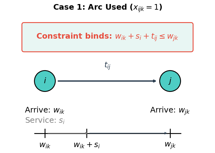
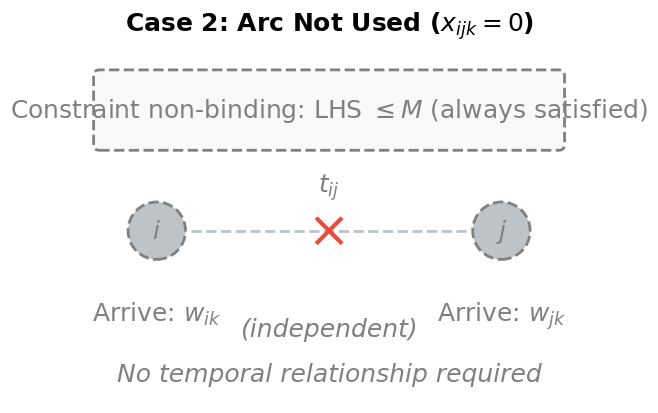
The diagram above makes the Big-M mechanism visible. The key insight is that this single constraint accomplishes two things: it enforces physical causality when routes are used, while remaining "invisible" for routes that don't exist in the solution. This conditional behavior is what makes Big-M constraints effective for modeling conditional relationships in optimization problems.
Constraint 6: The Binary Domain
The requirement: Routing decisions must be discrete: either a vehicle takes an arc, or it doesn't.
where:
- : the routing decision variable for arc and vehicle
- : the binary domain (variable can only take value 0 or 1)
- : set of all arcs
- : set of all vehicles
This might seem like a trivial "constraint," but it's actually what makes VRPTW computationally challenging. If we allowed to take any value between 0 and 1 (a "relaxation"), we could solve the problem much faster using continuous optimization techniques. A solution might say "send 0.3 of a vehicle from A to B," which is mathematically valid but operationally meaningless.
The binary requirement forces discrete decisions: a truck either takes a road or it doesn't. There's no "half a route." This discreteness is what transforms a tractable linear program into the NP-hard mixed-integer program that VRPTW is known to be.
Seeing the System: How Constraints Interact
We've now developed six constraints, but they don't operate in isolation. They form an interconnected system where a change in one part ripples through the others. Understanding this interaction is key to understanding why VRPTW is both powerful and challenging.
The Two Decision Dimensions:
Our model has two types of decision variables that the solver must determine simultaneously:
| Variable | Type | Dimension | Role |
|---|---|---|---|
| Binary | Spatial | Defines the route structure | |
| Continuous | Temporal | Defines when events happen |
These two dimensions are coupled through the precedence constraint (Big-M): the route structure determines which temporal relationships must hold.
The Constraint Ecosystem:
Think of the constraints as forming an ecosystem where each one addresses a potential failure mode:
- Service coverage ensures no customer is forgotten
- Capacity limits prevent physical overloading
- Flow conservation ensures routes are connected paths
- Time windows honor customer requirements
- Temporal precedence links space and time
- Binary domain forces discrete decisions
The solver's task is to find values for all variables that satisfy every constraint simultaneously while minimizing total cost. This is like solving a puzzle where each piece constrains what other pieces can be, except this puzzle has an exponentially large number of possible configurations.
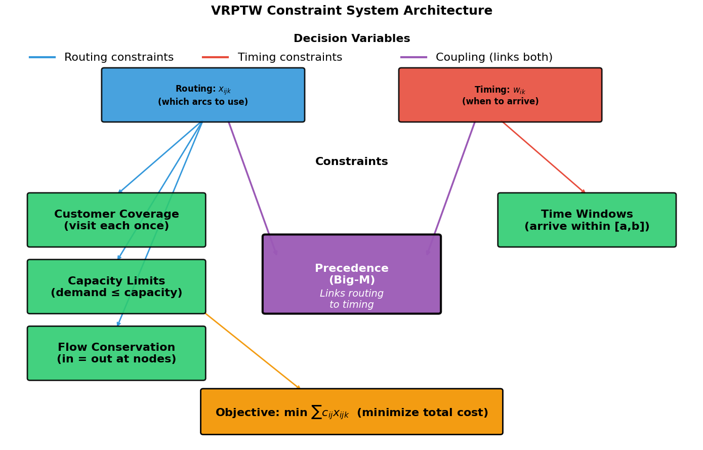
The diagram above visualizes this architecture. Notice how the routing variables () flow downward into spatial constraints (coverage, capacity, flow), while timing variables () connect to temporal constraints (time windows). The precedence constraint sits at the center, serving as the bridge that couples these two worlds. This coupling is what makes VRPTW fundamentally more challenging than solving routing and scheduling as separate problems. The two dimensions must be optimized jointly.
The Computational Challenge: Why VRPTW Is Hard
Having built our mathematical model, we should understand what we're asking a computer to do when we hand it this formulation.
The Curse of Combinatorics:
VRPTW inherits its difficulty from the Traveling Salesman Problem (TSP), which asks: "What's the shortest route visiting cities exactly once?" TSP is NP-hard, meaning no known algorithm can solve all instances quickly. VRPTW is strictly harder: it's TSP with additional constraints layered on top.
Consider the size of the search space for a modest problem with customers and vehicles:
| Decision | Possibilities | Growth Rate |
|---|---|---|
| Assign customers to vehicles | Partition items into groups | Exponential in |
| Sequence within each route | Order customers on each vehicle | Factorial per route |
| Time each arrival | Choose satisfying windows | Continuous but constrained |
For 20 customers and 3 vehicles, there are roughly possible customer-vehicle assignments, and for each assignment, we must consider many possible orderings. The total number of potential solutions dwarfs the number of atoms in the observable universe for even moderately sized problems.
Why We Need Sophisticated Algorithms:
Enumeration (checking every possible solution) is clearly infeasible. Instead, modern solvers employ clever strategies:
- Branch-and-bound: Systematically explore the solution space while pruning branches that can't lead to optimal solutions
- Constraint propagation: Use constraints to eliminate infeasible variable values early
- Metaheuristics: Use local search, simulated annealing, or genetic algorithms to find good (if not optimal) solutions quickly
- Hybrid approaches: Combine exact methods with heuristics for the best of both worlds
The mathematical formulation we've developed is the foundation upon which all these algorithms operate. It precisely defines what we're looking for. The algorithms provide strategies for finding it.
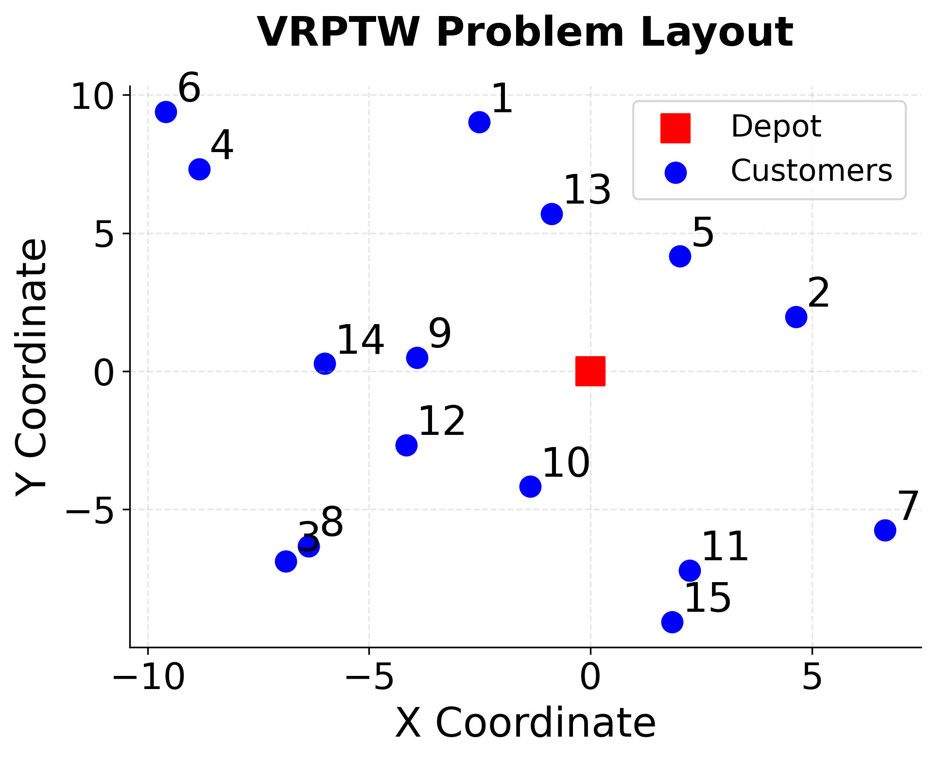
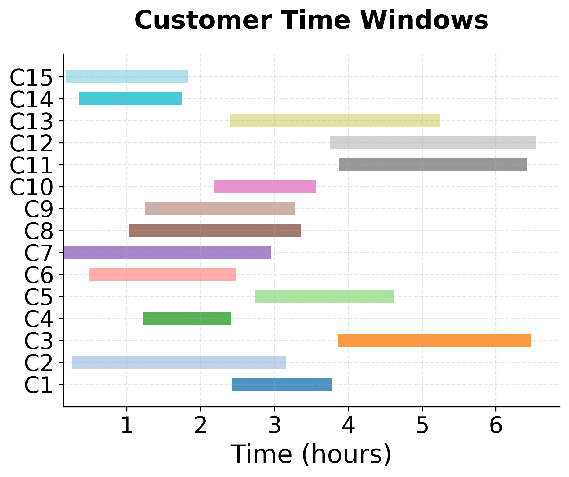
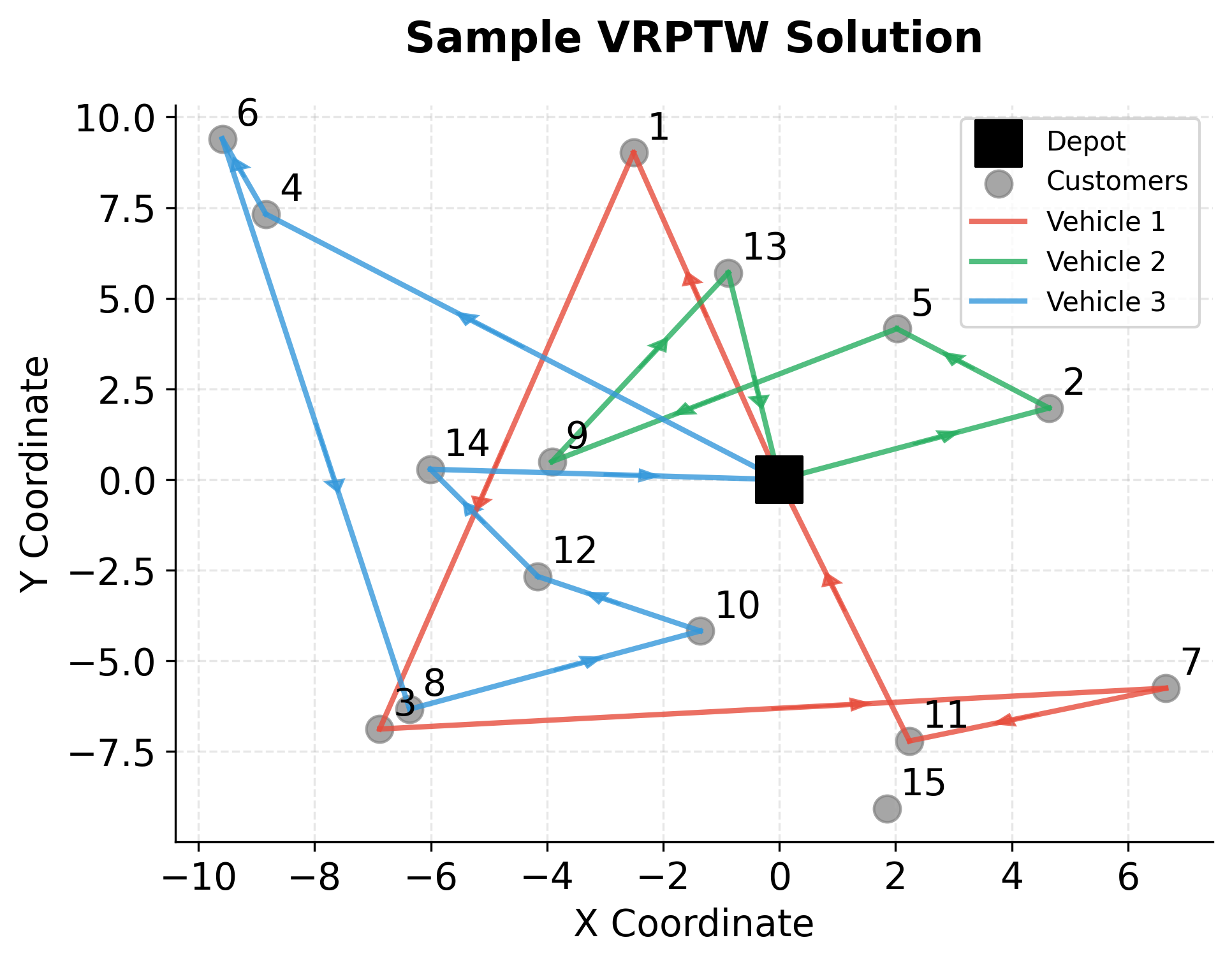
Visualizing VRPTW
Let's create visualizations to understand the VRPTW problem structure and solution characteristics.
Example
Now let's see how the mathematical formulation works in practice by solving a small, concrete example. This hands-on walkthrough will help you understand how the constraints interact and how a valid solution satisfies all requirements simultaneously.
Problem Setup: A Simple Delivery Scenario
Imagine you run a small delivery service with:
- 1 depot (your warehouse, location 0)
- 4 customers (locations 1-4) needing deliveries
- 2 vehicles, each with capacity 10 units
Each customer has specific requirements: a demand (how much they need), a time window (when they can receive delivery), and travel times between locations. Let's examine the data:
Key observations from the data:
- Customer 1 has the earliest time window (1-4) and is closest to the depot (travel time 2)
- Customer 4 has the latest time window (4-7) and is farthest from the depot (travel time 5)
- Total demand is 3+2+4+3 = 12 units, which exceeds either vehicle's capacity (10), so we need both vehicles
- The time windows overlap, creating flexibility in sequencing
Building a Solution: Step-by-Step Constraint Checking
Let's construct a feasible solution manually, checking each constraint as we go. This demonstrates how the mathematical formulation translates to practical routing decisions.
Step 1: Assigning Customers to Vehicles
We need to partition the 4 customers between 2 vehicles. Let's try:
- Vehicle 1: Customers 1 and 3 (demands: 3 + 4 = 7 units)
- Vehicle 2: Customers 2 and 4 (demands: 2 + 3 = 5 units)
Capacity check (Constraint 2):
- Vehicle 1: 7 ≤ 10
- Vehicle 2: 5 ≤ 10
Both assignments satisfy capacity constraints. Now we need to determine the sequence of visits for each vehicle.
Step 2: Sequencing Visits for Vehicle 1
Vehicle 1 must visit Customers 1 and 3. Let's consider the sequence: Depot → Customer 1 → Customer 3 → Depot
Time window check (Constraints 4 and 5):
Let's trace the route step by step, using our notation:
- Start at depot: (vehicle 1 starts at depot at time 0)
- Travel to C1: (travel time from depot to customer 1)
- Arrival at C1:
- Time window check: (Constraint 4 satisfied)
- Service at C1: (assume 0 service time for simplicity)
- Travel to C3: (travel time from customer 1 to customer 3)
- Arrival at C3:
- Time window check: (Constraint 4 satisfied)
- Precedence check: (Constraint 5 satisfied)
- Return to depot: (travel time from customer 3 to depot)
- Arrival at depot:
Flow conservation check (Constraint 3):
- Vehicle 1 enters C1: 1 arc (from depot)
- Vehicle 1 leaves C1: 1 arc (to C3)
- Vehicle 1 enters C3: 1 arc (from C1)
- Vehicle 1 leaves C3: 1 arc (to depot)
Route 1 is feasible! In terms of our decision variables:
- (vehicle 1 travels depot→C1)
- (vehicle 1 travels C1→C3)
- (vehicle 1 travels C3→depot)
- , (arrival times)
Step 3: Sequencing Visits for Vehicle 2
Vehicle 2 must visit Customers 2 and 4. Let's try: Depot → Customer 2 → Customer 4 → Depot
Time window check:
Tracing route 2 with our notation:
- Start at depot: (vehicle 2 starts at depot at time 0)
- Travel to C2: (travel time from depot to customer 2)
- Arrival at C2:
- Time window check: (Constraint 4 satisfied)
- Service at C2: (assume 0 service time)
- Travel to C4: (travel time from customer 2 to customer 4, from distance matrix row 2, column 4)
- Arrival at C4:
- Time window check: (Constraint 4 satisfied)
- Precedence check: (Constraint 5 satisfied)
- Return to depot: (travel time from customer 4 to depot)
- Arrival at depot:
Route 2 is also feasible! Decision variables:
- , ,
- ,
Step 4: Verifying All Constraints
Let's verify that our complete solution satisfies all constraints:
Constraint 1 (Each customer visited exactly once):
For each customer , we verify:
- Customer 1 ():
(Only , all others are 0)
- Customer 2 ():
(Only )
-
Customer 3 ():
(Only )
-
Customer 4 ():
(Only )
Constraint 2 (Capacity):
For vehicle 1 ():
Since and (and all other for vehicle 1):
For vehicle 2 ():
Since and (and all other for vehicle 2):
Constraint 3 (Flow conservation): Already verified in Steps 2 and 3
Constraint 4 (Time windows): Already verified in Steps 2 and 3
Constraint 5 (Temporal precedence): Already verified in Steps 2 and 3
Constraint 6 (Binary variables): All are 0 or 1
Solution Summary
Our complete solution:
Route 1 (Vehicle 1): Depot → Customer 1 → Customer 3 → Depot
- Arcs used: , ,
- Travel time calculation:
- Demand served:
- Arrival times: (within window ), (within window )
Route 2 (Vehicle 2): Depot → Customer 2 → Customer 4 → Depot
- Arcs used: , ,
- Travel time calculation:
- Demand served:
- Arrival times: (within window ), (within window )
Total travel time (objective value):
where (using travel time as cost).
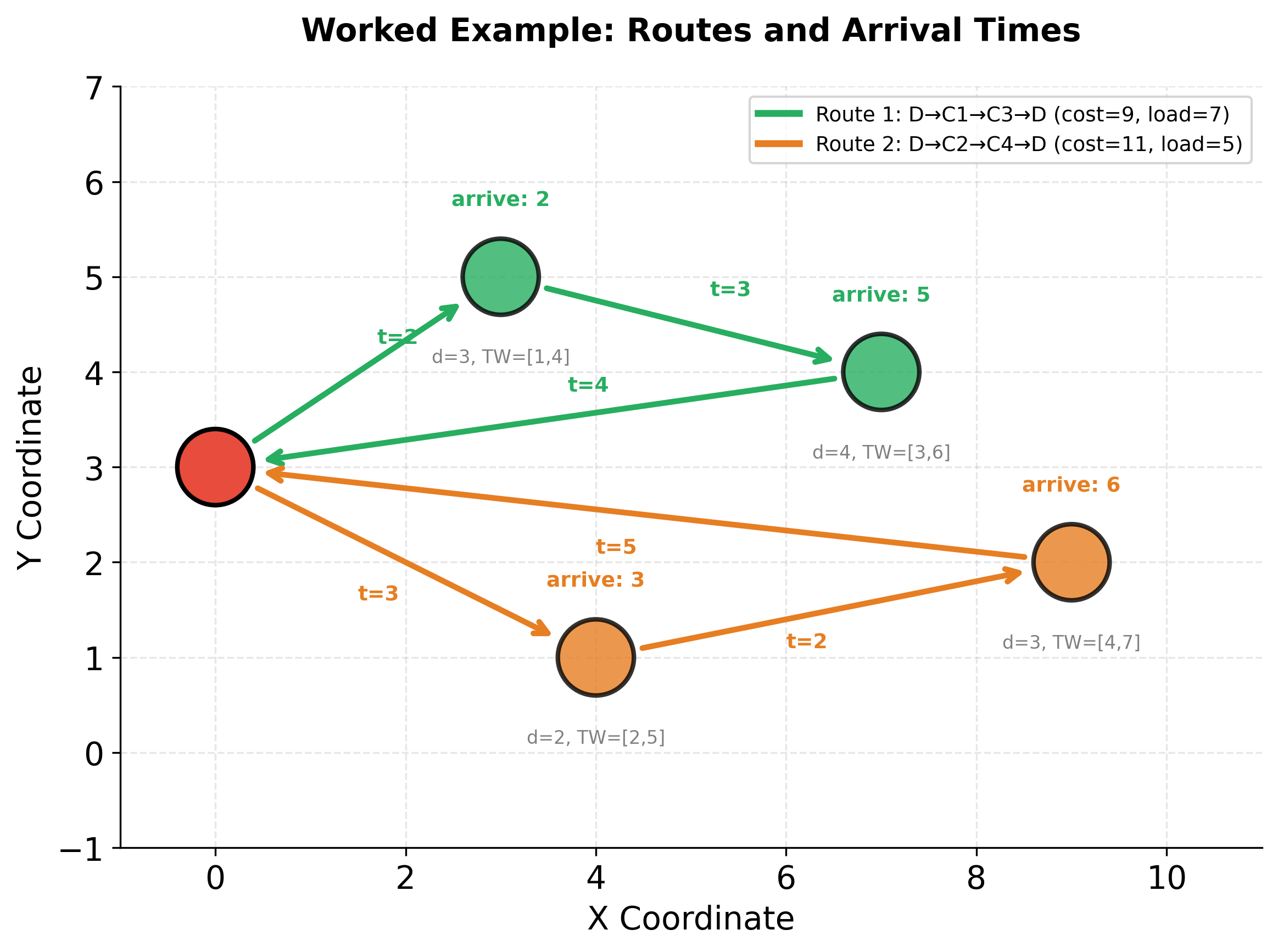

The visualizations above show the complete worked example. The first figure displays the spatial routes with travel times annotated on each arc, customer demands (d), and time windows (TW). The second figure shows the timeline for how each vehicle progresses through time, with shaded regions representing time windows and vertical bars marking actual arrival times. Notice how all arrivals fall within their respective time windows, confirming the solution's feasibility.
Why This Solution Works
This example illustrates several key insights:
-
Capacity constraints force customer partitioning: Since total demand (12) exceeds individual vehicle capacity (10), we need to use both vehicles. The capacity constraint guides how we group customers.
-
Time windows influence sequencing: Customer 1's early window (1-4) makes it a natural first stop. Customer 4's later window (4-7) provides flexibility for later visits.
-
Travel times affect feasibility: The sequence C1→C3 works because travel time 3 allows arrival at C3 (time 5) within its window [3,6]. A different sequence might violate time windows.
-
Constraints are interdependent: We can't optimize routes independently. The capacity constraint affects which customers can be grouped, which affects sequencing options, which affects time window feasibility.
This small example demonstrates the complexity that emerges even with just 4 customers. Real-world problems with hundreds of customers require sophisticated algorithms to navigate this constraint space efficiently.
Implementation in Google OR-Tools
Now that we understand the mathematical formulation and have worked through a manual example, let's see how to implement VRPTW using Google OR-Tools. This implementation translates our mathematical constraints into code, allowing the solver to automatically find optimal or near-optimal solutions.
From Mathematics to Code: Mapping Constraints
OR-Tools uses a constraint programming approach that implements our mathematical formulation through "dimensions" and "callbacks." Each constraint from our formulation maps to specific OR-Tools constructs:
- Routing decisions (): Handled automatically by the routing model's internal variables
- Time tracking (): Implemented through a "Time" dimension
- Capacity constraints: Implemented through a "Capacity" dimension
- Time windows: Set as bounds on the Time dimension
- Flow conservation: Enforced automatically by the routing model structure
Let's build the implementation step by step, connecting each code section to its corresponding mathematical concept.
We'll implement VRPTW step by step, starting with the data model and then building the solver configuration. This approach helps understand how each component maps to the mathematical formulation.
Now we'll create the solver function that implements all the constraints from our mathematical formulation:
Now let's solve the problem and extract the solution:
Display the solution results:
The objective value represents the sum of all arc costs used in the routes, corresponding to our mathematical objective function . The solution assigns customers to vehicles such that all capacity constraints are satisfied (each vehicle carries at most 8 units of demand) and all time windows are respected. Finding a feasible solution confirms that all constraints can be satisfied simultaneously for this problem instance.
Let's visualize the solution to see how vehicles are assigned to customers:
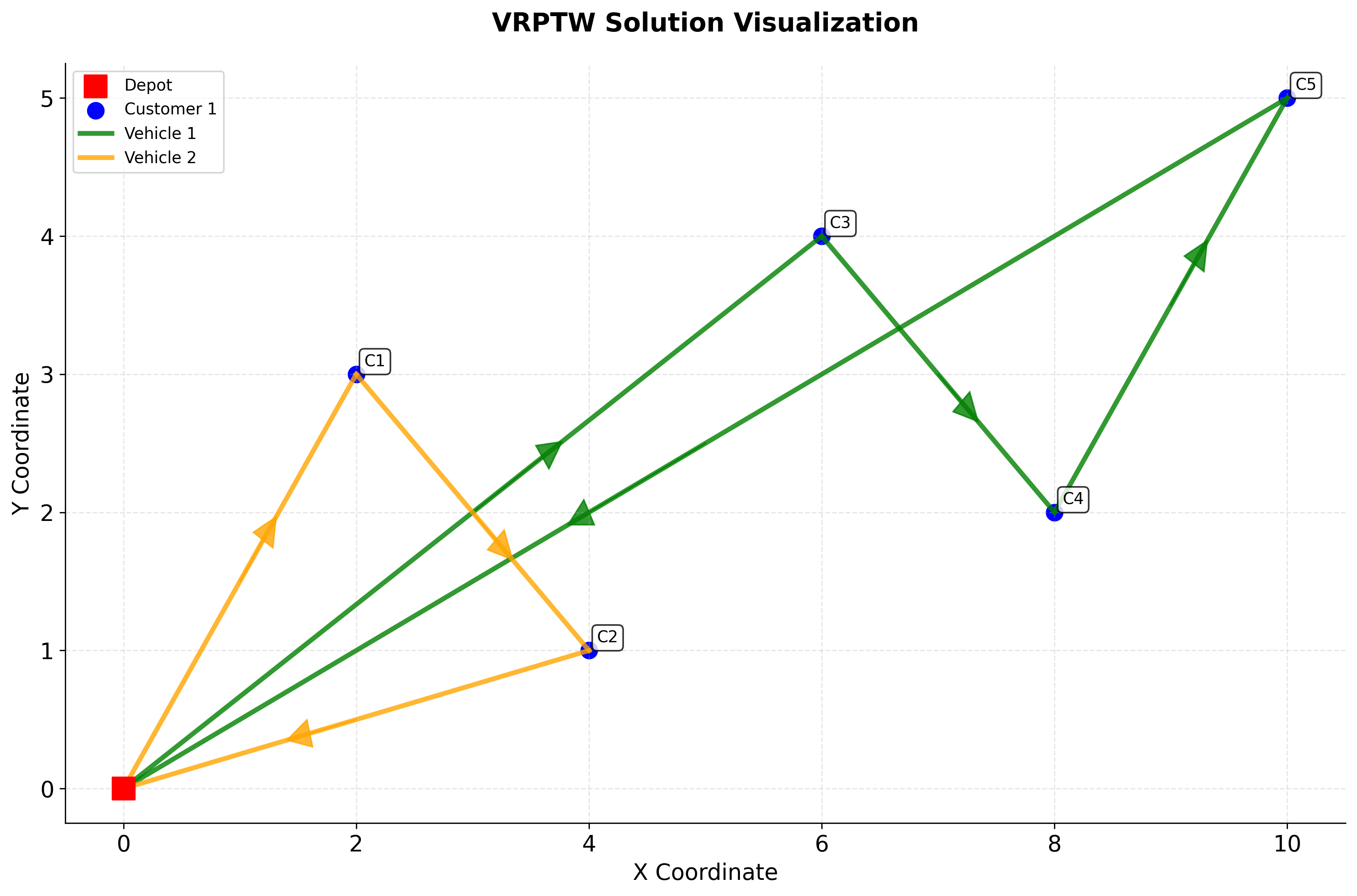
The visualization shows how vehicles are assigned to serve customers. Each colored line represents a vehicle's route, starting and ending at the depot (red square). The routes minimize total travel distance while respecting capacity constraints and time windows. Customers appearing on the same colored path are served by a single vehicle, demonstrating how the solver partitions customers across the fleet to achieve feasibility.
Alternative Implementation: Custom Heuristic
While OR-Tools uses sophisticated constraint programming to find optimal or near-optimal solutions, it's instructive to implement a simple greedy heuristic. This approach makes decisions sequentially rather than exploring the full solution space, and it helps illustrate how the constraints guide decision-making. The heuristic doesn't explicitly solve for all variables simultaneously; instead, it builds routes incrementally, checking constraints as it goes. This is much faster but may not find optimal solutions.
The heuristic still respects the same constraints: each customer is visited exactly once (by construction), capacity limits are checked before adding customers, time windows are verified before assignment, and temporal logic is maintained through arrival time tracking.
Display the heuristic solution and compare with OR-Tools:
The greedy heuristic builds routes incrementally by always choosing the nearest feasible customer. The key insight is that vehicles can wait if they arrive before a time window opens, so early arrival doesn't disqualify a customer. At each step, the algorithm checks: (1) capacity constraints, (2) time window feasibility, and (3) whether the vehicle can return to the depot on time after serving the customer.
Comparing the heuristic to OR-Tools reveals the cost of greedy decision-making. The heuristic finds a feasible solution quickly but typically produces routes that are longer than optimal. This is because locally optimal choices (picking the nearest customer) don't always lead to globally optimal solutions. OR-Tools explores the full solution space using constraint propagation and metaheuristics, finding better route combinations that the greedy approach misses.
Key Parameters
Below are the main parameters that affect how the VRPTW solver works and performs.
-
first_solution_strategy: Heuristic for generating the initial solution.PATH_CHEAPEST_ARC(default) builds routes by selecting the cheapest arc at each step.SAVINGSuses Clarke-Wright savings algorithm.CHRISTOFIDESuses Christofides algorithm for TSP components. -
local_search_metaheuristic: Metaheuristic for improving the initial solution.GUIDED_LOCAL_SEARCH(recommended) balances exploration and exploitation.TABU_SEARCHavoids revisiting solutions.SIMULATED_ANNEALINGprobabilistically accepts worse solutions to escape local optima. -
time_limit.seconds: Maximum solver time (default: unlimited). Use 30-60 seconds for 50-100 customers, 2-5 minutes for larger problems, 10-30 seconds for real-time dispatch. -
vehicle_capacities: List of capacity limits per vehicle. Supports homogeneous (all same) or heterogeneous fleets. Total capacity must exceed total customer demand. -
distance_matrix: Travel times or distances between all locations. Use actual road network values rather than Euclidean distances. Should be symmetric for undirected problems. -
time_windows: Tuples(earliest, latest)defining for each location. Depot window defines operational hours. Customer windows must be reachable from depot. -
service_times: Duration spent at each location (excluding travel). Use realistic estimates. Underestimating causes downstream time window violations. Depot service time is typically 0. -
demands: Demand at each location. Depot has demand 0. Total demand should be less than total vehicle capacity with margin.
Key Methods
The following are the most commonly used methods for working with OR-Tools routing models.
-
RoutingIndexManager(num_nodes, num_vehicles, depot): Creates an index manager mapping between node indices and routing indices. The depot (typically 0) serves as start/end point for all routes. -
RoutingModel(manager): Creates the main routing model that manages decision variables and constraints. -
RegisterTransitCallback(callback): Registers a binary callback returning cost/time to travel between two nodes. Used for distance and time dimensions. -
RegisterUnaryTransitCallback(callback): Registers a unary callback for single-node operations like demand pickup. Used for capacity dimensions. -
AddDimension(callback, slack_max, capacity, fix_start_cumul_to_zero, name): Adds a cumulative dimension (time, capacity) to the model. The callback defines accumulation; slack_max and capacity define bounds. -
AddDimensionWithVehicleCapacity(callback, slack, capacities, fix_start_cumul_to_zero, name): LikeAddDimensionbut with per-vehicle capacity limits. Use for heterogeneous fleets. -
SolveWithParameters(search_parameters): Solves the problem with specified search parameters. Returns solution object orNoneif infeasible. -
solution.ObjectiveValue(): Returns the objective value (total cost) of the solution: . -
solution.Value(routing.NextVar(index)): Returns the next node in the route. Use to trace complete routes for each vehicle.
Practical Implications
VRPTW addresses logistics scenarios where customers have specific availability windows that constrain when service can occur. This makes it appropriate for last-mile delivery operations, field service scheduling, healthcare logistics, and any routing problem where temporal constraints are binding rather than advisory. The formulation captures the core tradeoff between route efficiency and schedule adherence that characterizes modern logistics operations.
The approach is most valuable when time windows represent hard constraints, situations where arriving outside the window is genuinely infeasible rather than merely undesirable. Examples include scheduled appointment services, store receiving hours, and perishable goods delivery where timing affects product quality. When time windows are soft (violations incur penalties but are permitted), the standard VRPTW formulation requires modification to include penalty terms in the objective function. For problems without meaningful temporal constraints, simpler VRP variants will be more appropriate and computationally tractable.
Consider the density and overlap of time windows when assessing problem suitability. Problems with highly restrictive, non-overlapping windows may have few or no feasible solutions, while problems with very wide windows offer little value from the time window constraint and may be better modeled as basic VRP. The interaction between window tightness and geographic dispersion determines problem difficulty: clustered customers with overlapping windows are easier than dispersed customers with tight, disjoint windows.
Best Practices
Configure OR-Tools with PATH_CHEAPEST_ARC as the initial solution strategy and GUIDED_LOCAL_SEARCH as the metaheuristic for general-purpose VRPTW solving. For problems dominated by capacity constraints, consider SAVINGS instead. Set time_limit.seconds based on operational requirements: 30-60 seconds provides good solutions for 50-100 customer problems, while 2-5 minutes yields near-optimal solutions for batch planning. Real-time dispatch applications may need 10-30 second limits, accepting some solution quality degradation.
Validate problem feasibility before invoking the solver by checking that total demand does not exceed total vehicle capacity and that each customer can be reached from the depot within its time window. This prevents wasted computation on infeasible instances. For problems exceeding 100 customers, apply geographic clustering or time-window-based partitioning to decompose the problem into tractable subproblems. Solve subproblems independently, then optionally refine inter-cluster connections.
Use conservative service time estimates rather than optimistic ones. Underestimating service duration propagates delays through the route, causing downstream time window violations that may not appear until execution. When service times vary significantly, model the 75th-90th percentile duration rather than the mean.
Data Requirements and Preprocessing
The travel time matrix is the most critical input, as errors directly translate to infeasible solutions or poor execution. Use routing APIs or historical GPS data to estimate actual driving times rather than computing Euclidean or Manhattan distances. Traffic patterns vary by time of day, so consider using time-dependent travel times for problems spanning multiple hours. For problems with 100+ customers, the matrix requires storage; consider sparse representations or on-demand distance computation for larger instances.
Time window data must be validated against travel time feasibility. For each customer, verify that the depot-to-customer travel time allows arrival within the window, accounting for earliest departure from the depot. Similarly, check that customer-to-depot return is possible within operational hours. Customers failing these checks indicate data errors or require special handling (e.g., dedicated vehicles, earlier depot opening).
Demand data should sum to less than total vehicle capacity with reasonable margin. If total demand approaches total capacity, the problem becomes tightly constrained and may require all vehicles regardless of route efficiency. Service times should include all activities at the customer location: parking, walking, handoff, signature collection, and departure preparation. Depot service time is typically zero unless vehicles require loading or inspection.
Common Pitfalls
Relying on Euclidean distances for the travel matrix creates solutions that appear optimal but fail during execution. Road networks, traffic lights, and restricted turns can double or triple actual travel time compared to straight-line distance. Validate computed routes against actual driving times for a sample of arcs and adjust the matrix if systematic errors exist.
Setting time windows without considering travel time dependencies creates infeasible instances. If customer A's window closes at 10:00 and customer B's window opens at 10:15, but travel between them requires 30 minutes, no single vehicle can serve both. These hidden conflicts may not be obvious until the solver reports infeasibility or produces poor solutions.
Ignoring service time variability leads to optimistic schedules. If actual service takes longer than modeled, delays accumulate along the route. A 5-minute underestimate at each of 8 customers creates 40 minutes of delay by route end. Model conservatively, especially for variable-duration services like installation or repair.
Computational Considerations
VRPTW solution time grows exponentially with problem size due to NP-hardness. Practical scaling guidelines:
| Customer Count | Approach | Typical Time | Memory (Distance Matrix) |
|---|---|---|---|
| < 50 | Exact (branch-and-bound) | 1-5 minutes | < 10 KB |
| 50-100 | Heuristic (OR-Tools) | 30-120 seconds | < 40 KB |
| 100-200 | Heuristic with decomposition | 2-5 minutes | < 160 KB |
| 200-500 | Geographic partitioning | 5-15 minutes | < 1 MB |
| > 500 | Hierarchical approaches | 15+ minutes | 1+ MB |
The solver's memory footprint beyond the distance matrix is modest, typically under 100 MB for problems up to 500 customers. For larger problems, the primary bottleneck is solution time rather than memory. Decomposition strategies (clustering customers by location or time window) offer the best path to scaling, as they convert one large problem into several smaller, independently solvable problems.
Performance and Deployment Considerations
Evaluate solutions using multiple metrics: total travel distance (efficiency), number of vehicles used (resource utilization), time window adherence rate (service quality), and computation time (responsiveness). No single metric captures solution quality. A solution minimizing distance may require more vehicles; one using fewer vehicles may have tighter timing margins.
Production systems should distinguish batch and real-time scenarios. Batch planning (overnight route computation) can allocate 5-10 minutes per solve for near-optimal solutions. Real-time dispatch (responding to new orders) needs 10-30 second limits, using incremental re-optimization that modifies existing routes rather than solving from scratch.
Implement solution validation before deployment: programmatically verify that each route satisfies capacity constraints, arrives within time windows, and allows timely depot return. Solvers occasionally return solutions that violate constraints due to numerical issues or callback errors. For robustness, maintain fallback strategies when the solver fails. Options include relaxing the tightest time windows, deploying additional vehicles, or flagging problematic customers for manual handling.
Summary
The Vehicle Routing Problem with Time Windows represents a critical optimization challenge in modern logistics, balancing operational efficiency with customer service requirements. Through mathematical formulation and advanced optimization techniques, we can find solutions that minimize travel costs while respecting vehicle capacity and time window constraints.
Google OR-Tools provides powerful, accessible tools for solving VRPTW problems, making advanced optimization techniques available to practitioners without deep expertise in operations research. The combination of exact methods for smaller problems and heuristic approaches for larger instances enables practical application across various industries and problem sizes.
Successful VRPTW implementation requires careful attention to data quality, system integration, and ongoing optimization. The mathematical foundation provides a solid basis for understanding problem complexity, while modern computational tools make practical application feasible for real-world logistics operations.
Quiz
Ready to test your understanding? Take this quick quiz to reinforce what you've learned about the Vehicle Routing Problem with Time Windows.

Comments