InteractiveBM25: Complete Guide to the Search Algorithm Behind Elasticsearch

BM25Link Copied

BM25 (Best Matching 25) is the algorithm that powers search engines like Elasticsearch, Solr, and Lucene. It's been a standard in information retrieval since the 1990s and remains widely used today, even as neural approaches have emerged. Understanding BM25 gives you insight into what makes search actually work.

In this chapter, you'll learn where BM25 comes from (hint: probability theory), why it consistently outperforms TF-IDF, and how to implement it from scratch. We'll also explore its variants and see empirically how it stacks up against simpler approaches.

The Probabilistic FoundationLink Copied

BM25 didn't emerge from nowhere. It's the result of decades of research in probabilistic information retrieval, a field that asks: given a query, what's the probability that a document is relevant?

The Binary Independence ModelLink Copied

The story begins with the Binary Independence Model (BIM), developed in the 1970s. BIM makes two key assumptions:

1. Binary: Each term either appears in a document or it doesn't (we ignore term frequency)
2. Independence: Terms occur independently of each other given the relevance of a document

Under BIM, we want to rank documents by $P(R|D,Q)$, the probability that document $D$ is relevant given query $Q$. Using Bayes' theorem and the independence assumption, this leads to ranking by:

where:

• $t$: a term in both the query and document
• $Q \cap D$: the set of terms appearing in both query $Q$ and document $D$
• $P(t|R)$: probability of term $t$ appearing in a relevant document
• $P(t|\bar{R})$: probability of term $t$ appearing in a non-relevant document

The problem? We rarely have relevance judgments to estimate these probabilities. Robertson and Spärck Jones showed that with some simplifying assumptions, this reduces to something familiar: inverse document frequency.

From BIM to BM25Link Copied

The Binary Independence Model ignores term frequency entirely, which is clearly a limitation. If a document mentions "machine learning" ten times, that should matter more than mentioning it once.

Robertson and Walker addressed this in the 1990s through a series of papers that culminated in BM25. The key insight was to incorporate term frequency in a principled way while maintaining the probabilistic foundation.

The derivation involves the 2-Poisson model, which assumes that term frequencies in relevant and non-relevant documents follow different Poisson distributions. Working through the math (which we'll spare you), this leads to a term frequency weighting that saturates, meaning additional occurrences of a term provide diminishing returns.

The BM25 FormulaLink Copied

The full BM25 formula looks intimidating at first glance, but every piece exists for a reason. Rather than presenting it all at once, let's build it up from the three core problems any good retrieval function must solve:

1. Which terms matter? Not all words are equally informative. "The" appears everywhere; "quantum" is rare and specific.
2. How much does repetition help? If a document mentions your query term once, that's good. But is mentioning it 100 times really 100 times better?
3. How do we handle document length? A 10,000-word document naturally contains more vocabulary than a 100-word document. Should we penalize it for that?

BM25 addresses each of these problems with a specific component. Let's examine them one by one, then see how they combine into the complete formula.

Problem 1: Which Terms Matter? The IDF ComponentLink Copied

Consider searching for "the cat sat on the mat." The word "the" appears in virtually every English document. Finding it tells you almost nothing. But "mat"? That's much more specific.

The Inverse Document Frequency (IDF) quantifies this intuition. A term that appears in many documents gets a low IDF; a rare term gets a high IDF. BM25 uses a specific IDF formulation derived from its probabilistic foundations:

where:

• $N$: total number of documents in the collection
• $n(t)$: number of documents containing term $t$
• The $+0.5$ terms provide smoothing to avoid division by zero and extreme values

This formulation differs from the standard $\log(N/n(t))$ IDF you might have seen elsewhere. The $N - n(t)$ in the numerator comes directly from the probabilistic derivation, representing the number of documents that don't contain the term.

Here's the key insight: for very common terms appearing in more than half the documents, this IDF actually becomes negative. The formula effectively penalizes ubiquitous terms rather than just ignoring them. If a term appears in 80% of documents, matching on it might actually hurt your score slightly, pushing you to focus on more discriminative terms.

Let's visualize how IDF varies with document frequency:

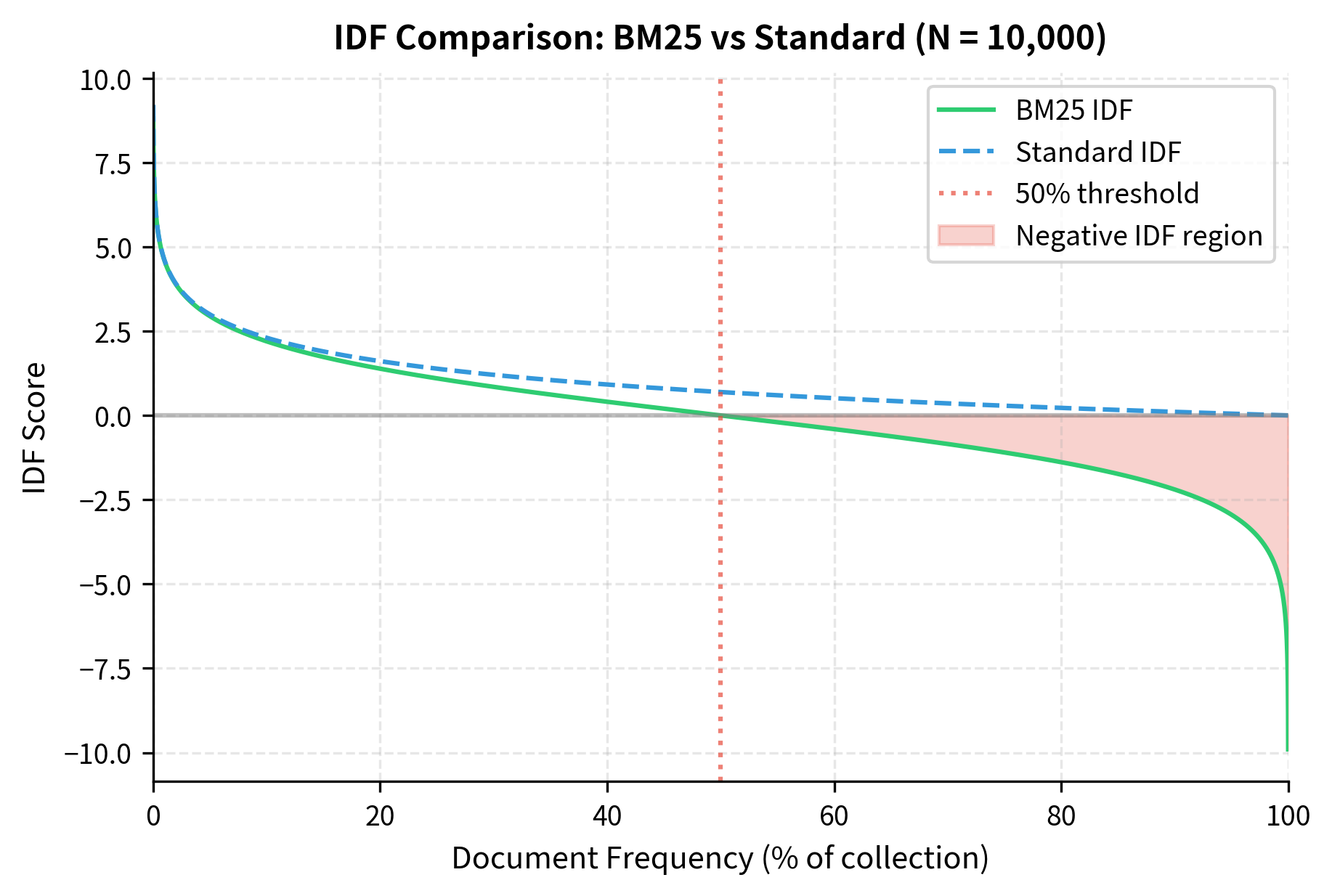
The plot reveals an important difference: standard IDF is always positive, merely approaching zero for common terms. BM25's IDF crosses zero at exactly 50% document frequency and becomes increasingly negative beyond that. This means stopwords like "the" or "a" that appear in nearly every document will have strongly negative IDF, effectively penalizing documents that match only on these terms.

Problem 2: How Much Does Repetition Help? The Saturation EffectLink Copied

If a document mentions "machine learning" once, that's evidence of relevance. What about ten times? A hundred times?

Raw term frequency treats each occurrence equally: ten mentions = ten times the score. But this creates problems. A document that repeats a term obsessively (keyword stuffing) would dominate results. More fundamentally, there's a diminishing returns effect: the first mention tells you the document is about the topic; additional mentions provide less and less new information.

BM25 captures this with a saturation function:

where $f(t, D)$ is the frequency of term $t$ in document $D$, and $k_1$ is a parameter controlling saturation speed. (The full formula includes length normalization in the denominator, which we'll add shortly.)

To understand why this formula creates saturation, consider what happens as $f(t, D)$ grows very large. The numerator grows linearly, but the denominator grows at the same rate. In the limit, the ratio approaches $k_1 + 1$, an asymptote that cannot be exceeded no matter how many times the term appears.

The parameter $k_1$ controls how quickly you approach this ceiling:

• $k_1 = 0$: Instant saturation. Any non-zero term frequency gives the same score (like the Binary Independence Model)
• $k_1 \to \infty$: No saturation. Score is linear in term frequency (like raw TF-IDF)
• $k_1 \approx 1.2$ to $2.0$: The empirically validated sweet spot for most collections

Let's visualize this saturation effect:

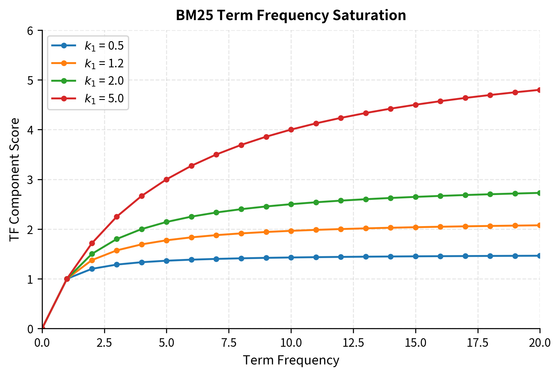
The visualization reveals the saturation behavior clearly. With $k_1 = 0.5$, the curve flattens quickly: by term frequency 5, you've captured most of the possible score. With $k_1 = 5.0$, the curve is nearly linear over this range, meaning repetition continues to help. The default value of $k_1 = 1.2$ provides a principled middle ground: the first few occurrences matter a lot, but the score doesn't keep climbing indefinitely.

Problem 3: How Do We Handle Document Length?Link Copied

Here's a subtle but important issue. Imagine two documents about machine learning:

• Document A: A focused 200-word abstract that mentions "neural network" twice
• Document B: A comprehensive 10,000-word survey that mentions "neural network" twenty times

Which is more relevant to a query about neural networks? Raw term frequency would strongly favor Document B. But that's not necessarily right. Document B mentions the term more often simply because it's longer. The density of the term, its frequency relative to document length, might be a better signal.

BM25 addresses this through length normalization, which adjusts term frequency based on how a document's length compares to the collection average:

where:

• $b$: length normalization parameter (0 to 1)
• $|D|$: length of document $D$ (number of terms)
• $\text{avgdl}$: average document length across the collection

This expression appears in the denominator of the BM25 formula, multiplied by $k_1$. For a document exactly at average length, the expression equals 1 (no adjustment). For longer documents, it's greater than 1, which increases the denominator and reduces the score. For shorter documents, it's less than 1, which decreases the denominator and increases the score.

The parameter $b$ controls how aggressively we normalize:

• $b = 0$: No length normalization. The expression always equals 1, and document length is ignored entirely.
• $b = 1$: Full length normalization. A document twice the average length has its term frequencies effectively halved.
• $b \approx 0.75$: The typical default, providing moderate normalization that accounts for length without completely eliminating its effect.

Let's see how length normalization affects scoring:

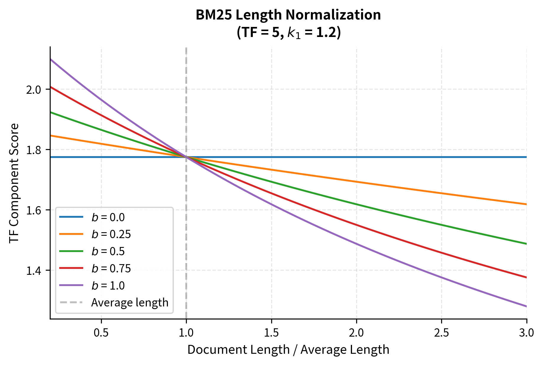
The visualization confirms our intuition. When $b = 0$, document length doesn't matter at all: all curves are flat. With $b = 1$, a document that's three times average length gets significantly penalized. The default $b = 0.75$ provides a reasonable middle ground, acknowledging that longer documents might naturally contain more occurrences without completely ignoring the length difference.

Putting It All Together: The Complete FormulaLink Copied

Now we can assemble the complete BM25 formula. For each query term, we multiply three components:

1. IDF: How informative is this term?
2. Saturated TF: How often does it appear (with diminishing returns)?
3. Length adjustment: Normalized by document length

The final formula sums these contributions across all query terms:

where:

• $D$: the document being scored
• $Q$: the query (set of query terms)
• $t$: a term in the query
• $\text{IDF}(t)$: inverse document frequency of term $t$
• $f(t, D)$: frequency of term $t$ in document $D$
• $k_1$: saturation parameter (typically 1.2 to 2.0)
• $b$: length normalization parameter (typically 0.75)
• $|D|$: length of document $D$ (number of terms)
• $\text{avgdl}$: average document length in the collection

Each component addresses one of our original problems. The IDF weights rare terms more heavily. The saturation function ensures diminishing returns from repetition. The length normalization factor in the denominator adjusts for document size. Together, they create a scoring function that has worked well across decades of information retrieval research.

Parameter Interaction: A Heatmap ViewLink Copied

The parameters $k_1$ and $b$ interact in interesting ways. Let's visualize how different combinations affect the score for a document with a fixed term frequency:

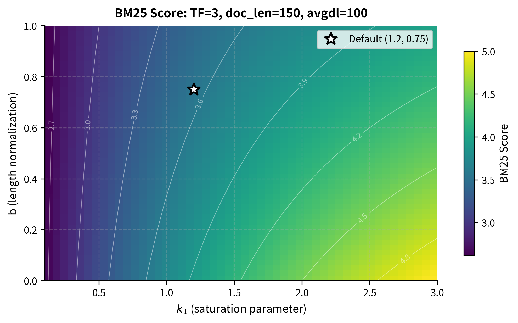
The heatmap reveals the parameter landscape. Moving right (higher $k_1$) increases scores because term frequency contributes more. Moving up (higher $b$) decreases scores because our document is longer than average and gets penalized more heavily. The default parameters sit in a region that balances these effects, but the optimal choice depends on your specific collection and retrieval goals.

A Worked ExampleLink Copied

With the formula understood, let's trace through a concrete example to see how all the pieces fit together. We'll score three short documents against a simple query, computing each component step by step.

Our corpus consists of three documents:

• D1: "the cat sat on the mat" (6 words)
• D2: "the cat sat on the cat mat" (7 words)
• D3: "the dog ran in the park" (6 words)

And our query is: "cat mat"

Notice that D1 and D2 both contain our query terms, but D2 mentions "cat" twice. D3 contains neither term. Let's see how BM25 handles these differences.

Step 1: Collection StatisticsLink Copied

Before scoring any document, we need collection-level statistics. These establish the baseline against which individual documents are compared:

We have 3 documents with an average length of about 6.3 words. Both "cat" and "mat" appear in 2 of the 3 documents. These statistics will feed into our IDF and length normalization calculations.

Step 2: Computing IDFLink Copied

Now let's compute the IDF for each query term. Remember, IDF measures how discriminative a term is. Terms appearing in fewer documents get higher IDF:

Both terms appear in 2 out of 3 documents, giving them identical IDF values of about -0.29. The negative IDF is notable: it means these terms are so common in our tiny corpus that they actually provide weak negative evidence. In a larger, more realistic corpus, query terms would typically have positive IDF values, but this example illustrates how the probabilistic derivation handles common terms.

Step 3: Scoring Each DocumentLink Copied

Now we combine everything: IDF, saturated term frequency, and length normalization. For each query term in each document, we compute the contribution and sum them up:

Let's visualize the score breakdown for each document to see how each query term contributes:

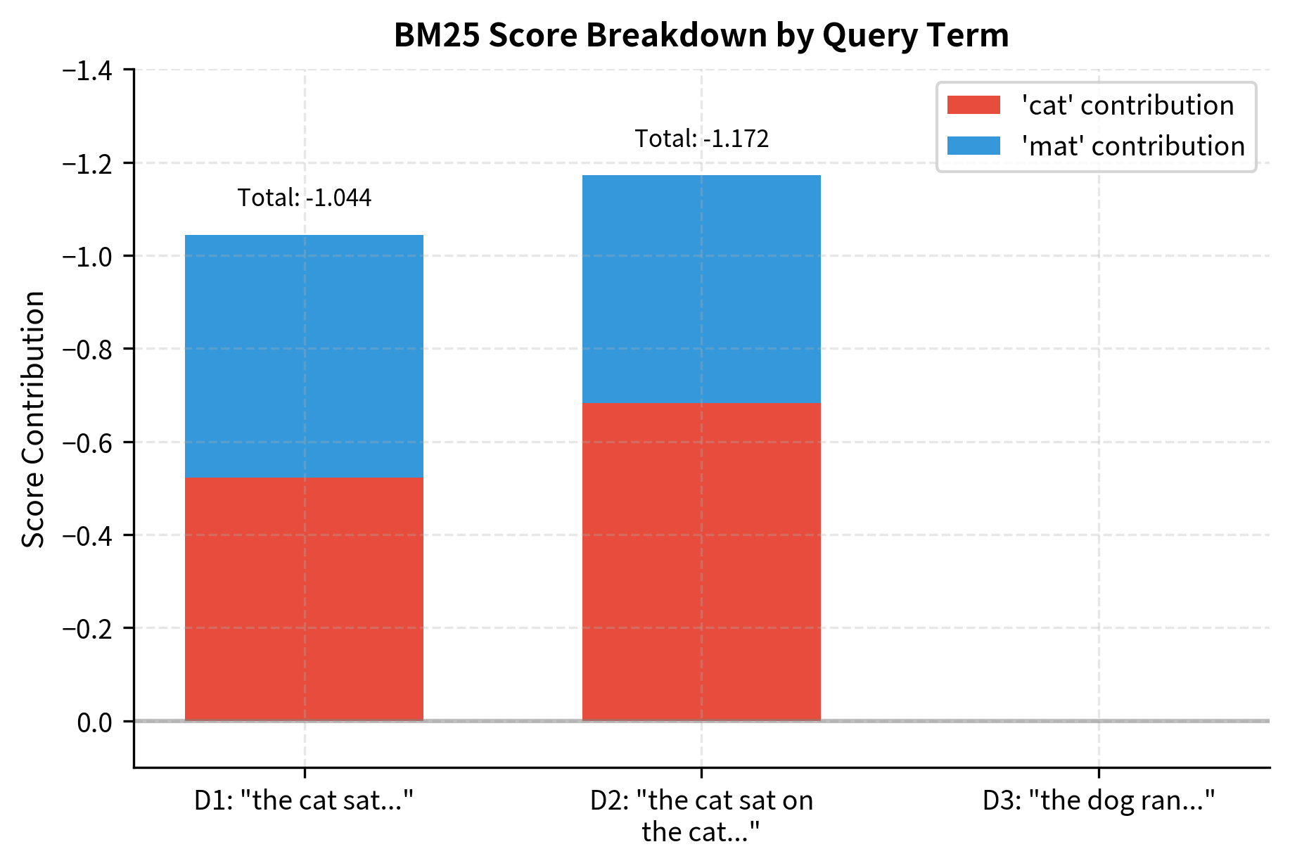
The visualization makes the scoring dynamics clear:

• D2 wins despite being the longest document. Why? It contains "cat" twice, and the saturation effect hasn't fully kicked in at TF=2. The extra occurrence still provides meaningful additional score.
• D1 comes second with both query terms appearing once each. It's slightly shorter than average, which gives it a small boost.
• D3 scores zero because it contains neither query term. No amount of length normalization or parameter tuning can help a document that lacks the query terms entirely.

The negative scores might seem strange, but they're a consequence of our small corpus where both query terms are common. In practice, with larger corpora and more discriminative query terms, you'd see positive scores. What matters is the relative ranking, and BM25 correctly identifies D2 as most relevant.

Implementing BM25 from ScratchLink Copied

Understanding the formula is one thing; implementing it efficiently is another. Let's build a complete BM25 retrieval system step by step, seeing how the mathematical concepts translate into code.

We'll use a larger corpus to make the results more interesting and realistic:

Building the IndexLink Copied

A BM25 index needs to store several pieces of information efficiently:

1. Document frequencies: For each term, how many documents contain it? (Needed for IDF)
2. Document lengths: How long is each document? (Needed for length normalization)
3. Average document length: The collection-wide baseline for length comparison
4. Inverted index: For each term, which documents contain it and with what frequency? (Needed for efficient retrieval)

Let's create a class that builds and stores this index:

The indexing process makes a single pass through the corpus, computing all the statistics we need. The inverted index is the key data structure for efficient retrieval: instead of scanning every document for each query, we can directly look up which documents contain each query term.

Implementing the Scoring FunctionLink Copied

Now we add methods to compute BM25 scores. The scoring function directly implements our formula, computing IDF, saturated term frequency, and length normalization for each query term:

Notice how the search method uses the inverted index to find candidate documents efficiently. Instead of scoring all documents, we only consider those containing at least one query term. This optimization matters for large corpora where most documents won't match the query at all.

Testing the ImplementationLink Copied

Let's test our BM25 implementation with several queries to see how it ranks documents:

Our BM25 implementation successfully retrieves relevant documents. Several patterns emerge from these results:

• Specific queries work well: "machine learning" finds the one document explicitly about ML and data science.
• Multiple matches boost scores: Documents matching both query terms (like "Python programming") score higher than those matching just one.
• IDF matters: Common terms like "programming" contribute less than rarer terms like "machine" or "enterprise."

The implementation is functionally complete, but production systems like Elasticsearch add many optimizations: compressed inverted indexes, skip lists for faster intersection, and caching of IDF values.

BM25 VariantsLink Copied

The original BM25 formula has some known issues that researchers have addressed with variants.

The Problem with Short DocumentsLink Copied

One issue with BM25 is that very short documents can be over-penalized. If a document is much shorter than average, the length normalization term $1 - b + b \cdot \frac{|D|}{\text{avgdl}}$ becomes less than 1, which actually boosts the term frequency component. But this boost might not be enough to compensate for the document simply having fewer terms.

BM25L: Lower Bound on TFLink Copied

BM25L (BM25 with Lower bound) addresses this by modifying how term frequency is normalized. First, it computes a length-normalized term frequency:

Then it adds a lower bound constant $\delta$ to this normalized value:

where:

• $c(t, D)$: length-normalized term frequency
• $\delta$: lower bound constant (typically 0.5)
• All other variables are the same as in standard BM25

The addition of $\delta$ to the normalized term frequency ensures that even a single occurrence of a term contributes meaningfully to the score, regardless of document length.

BM25+: Additive IDFLink Copied

BM25+ takes a different approach by adding a constant to the entire term weight:

where:

• $\delta$: additive constant (typically 1.0)
• All other variables are the same as in standard BM25

This guarantees that a document containing a query term always scores higher than one that doesn't, regardless of length normalization effects.

Let's compare these variants:

BM25+ consistently gives higher scores, especially for shorter documents where the additive $\delta$ term has more relative impact. BM25L provides a middle ground with its adjusted term frequency calculation.

Field-Weighted BM25Link Copied

Real documents often have structure: titles, abstracts, body text, metadata. A match in the title should probably count more than a match buried in the body. Field-weighted BM25 (sometimes called BM25F) addresses this.

The key idea is to compute a "virtual" term frequency that combines contributions from all fields:

where:

• $\tilde{f}(t, D)$: virtual (combined) term frequency for term $t$ in document $D$
• $c$: a field in the document (e.g., title, body, abstract)
• $w_c$: boost weight for field $c$ (higher values give more importance to matches in that field)
• $f(t, D_c)$: frequency of term $t$ in field $c$ of document $D$
• $b_c$: length normalization parameter specific to field $c$
• $|D_c|$: length of field $c$ in document $D$
• $\text{avgdl}_c$: average length of field $c$ across all documents

This virtual term frequency then plugs into a simplified BM25 formula (note that length normalization is already applied per-field in $\tilde{f}$):

Let's implement a simple version:

Let's test with structured documents:

Document 1 ranks highest because "Python" and "Programming" both appear in its title, which has 3x weight. Document 2 mentions "Python" only in the body (despite having "Development" in the title), so it ranks lower even though the body text is about Python.

BM25 vs TF-IDF: An Empirical ComparisonLink Copied

How much does BM25's sophistication actually matter? Let's compare it directly against TF-IDF on a retrieval task.

Now let's compare rankings for several queries:

The rankings often agree, but there are subtle differences. BM25's saturation effect means that a document with many occurrences of a query term doesn't dominate as much as it would with raw TF-IDF. The length normalization also helps ensure shorter, focused documents aren't overwhelmed by longer ones.

Let's visualize the score distributions:

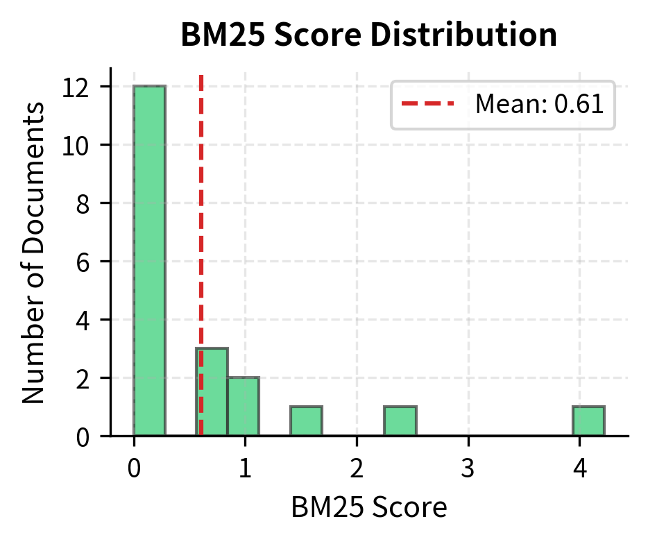
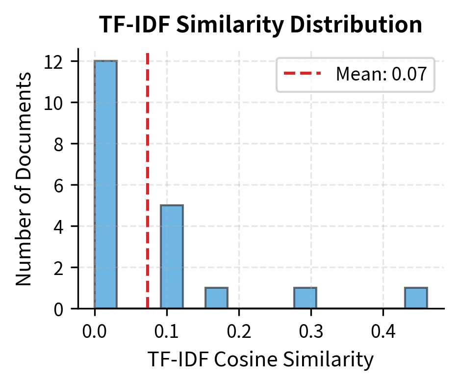
BM25 scores tend to have a wider dynamic range with clearer separation between relevant and non-relevant documents. TF-IDF cosine similarities are bounded between 0 and 1, which can make it harder to distinguish between moderately relevant documents.

Using BM25 in PracticeLink Copied

While understanding BM25 internals is valuable, in practice you'll often use existing implementations. The rank_bm25 library provides a simple, efficient implementation:

For production search systems, Elasticsearch and OpenSearch use BM25 as their default scoring algorithm. They also support BM25F for multi-field documents out of the box.

Limitations and Modern ContextLink Copied

BM25 works well in practice, but it has fundamental limitations:

Vocabulary mismatch: BM25 only matches exact terms. If your query says "car" but the document says "automobile," BM25 won't find the connection. Semantic search with embeddings handles this better.

No semantic understanding: "Bank of the river" and "Bank account" would be treated identically. BM25 has no concept of word meaning or context.

Bag of words assumption: Word order doesn't matter. "Dog bites man" scores the same as "Man bites dog" for a query about dogs and men.

Query-document length mismatch: Short queries searching long documents (or vice versa) can produce suboptimal results despite length normalization.

Despite these limitations, BM25 remains widely used because:

1. Speed: It's extremely fast, requiring only sparse vector operations
2. Interpretability: You can explain exactly why a document ranked where it did
3. No training required: It works out of the box on any text collection
4. Hybrid search: Modern systems often combine BM25 with neural retrievers, getting the best of both worlds

SummaryLink Copied

BM25 represents the high point of classical information retrieval. Its key innovations:

• Probabilistic foundation: Derived from principled probabilistic models, not ad-hoc heuristics
• Term frequency saturation: The $k_1$ parameter ensures diminishing returns from repeated terms
• Length normalization: The $b$ parameter prevents long documents from unfairly dominating
• IDF weighting: Rare terms receive higher weight, common terms are downweighted

The standard parameters ($k_1 = 1.2$, $b = 0.75$) work well across most collections, though tuning can help for specific domains. Variants like BM25L and BM25+ address edge cases with short documents, while BM25F handles structured documents with multiple fields.

BM25's lasting influence is evident in its continued use in Elasticsearch, Solr, and other search engines. Even as neural retrievers have emerged, BM25 often serves as a first-stage retriever or as part of hybrid systems. Understanding BM25 gives you insight into what makes search work, and why modern approaches needed to go beyond lexical matching to achieve true semantic understanding.

Key ParametersLink Copied

Understanding BM25's parameters is essential for tuning retrieval performance:

Tuning guidance:

• Start with defaults ($k_1 = 1.2$, $b = 0.75$): These work well for most text collections and are the defaults in Elasticsearch and Lucene.
• Increase $k_1$ (toward 2.0) when term frequency is highly informative, such as in longer documents where repeated mentions genuinely indicate relevance.
• Decrease $k_1$ (toward 0.5) for collections where a single mention is as informative as multiple mentions, such as short documents or when keyword stuffing is a concern.
• Decrease $b$ (toward 0.25) when document length variation is meaningful, for example, when longer documents genuinely contain more relevant information rather than just more filler.
• Increase $b$ (toward 1.0) when longer documents tend to match queries spuriously due to containing more vocabulary.
• Use BM25+ or BM25L when your collection has highly variable document lengths and you observe short, relevant documents being ranked too low.

QuizLink Copied

Ready to test your understanding? Take this quick quiz to reinforce what you've learned about BM25 and information retrieval.