

Learn how GloVe creates word embeddings by factorizing co-occurrence matrices. Covers the derivation, weighted least squares objective, and Python implementation.

This article is part of the free-to-read Language AI Handbook
Choose your expertise level to adjust how many terms are explained. Beginners see more tooltips, experts see fewer to maintain reading flow. Hover over underlined terms for instant definitions.
GloVe
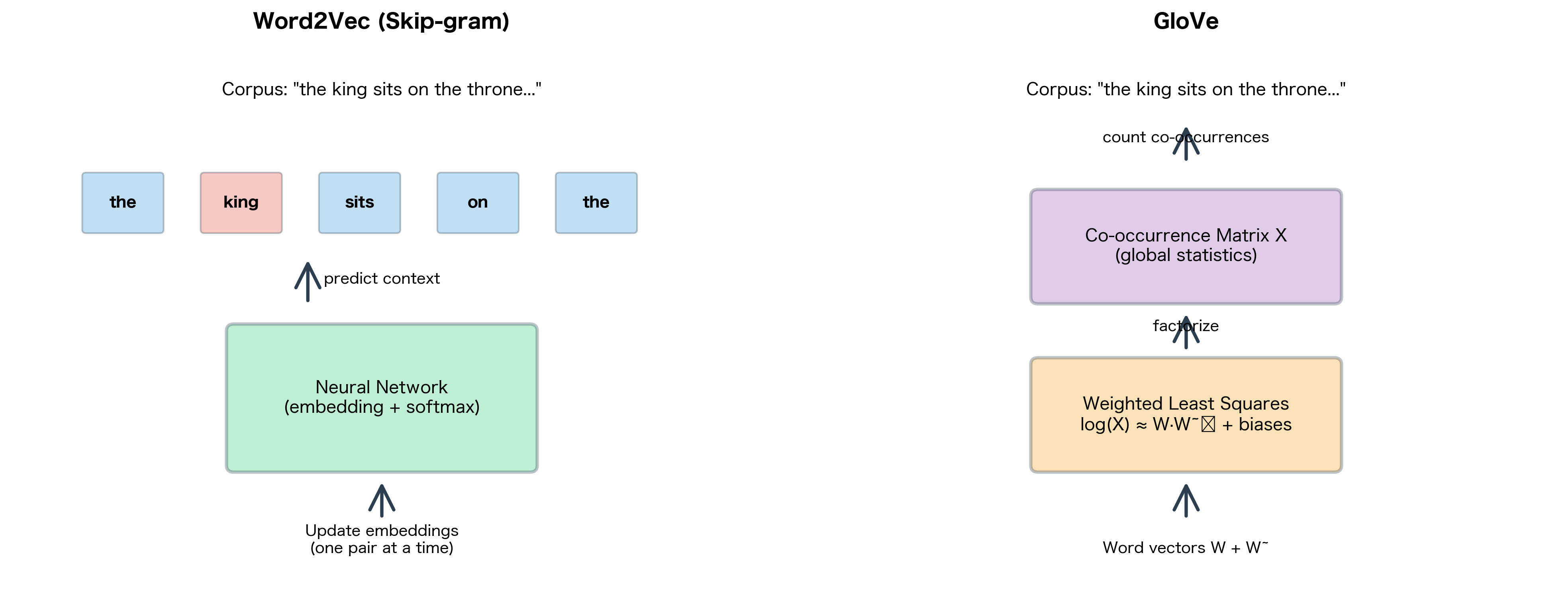
Word2Vec learns embeddings through local context windows, predicting surrounding words one pair at a time. This approach works well but ignores a fundamental insight: some word relationships are global properties of the corpus. The word "ice" might appear near "cold" millions of times across a billion-word corpus, but Word2Vec treats each occurrence as an independent prediction task. What if we could leverage this global co-occurrence information directly?
GloVe (Global Vectors for Word Representation) takes a different path. Developed by Pennington, Socher, and Manning at Stanford in 2014, GloVe starts with a co-occurrence matrix that captures how often words appear together across the entire corpus. It then factorizes this matrix to produce word vectors. The result: embeddings that encode both local context patterns and global corpus statistics.
This chapter develops GloVe from first principles. We'll see how the objective function emerges from a simple requirement that word vectors encode co-occurrence ratios, work through the weighted least squares formulation, and implement GloVe from scratch. By the end, you'll understand why GloVe achieves comparable results to Word2Vec despite taking a fundamentally different approach.
The Insight: Co-occurrence Ratios Reveal Meaning
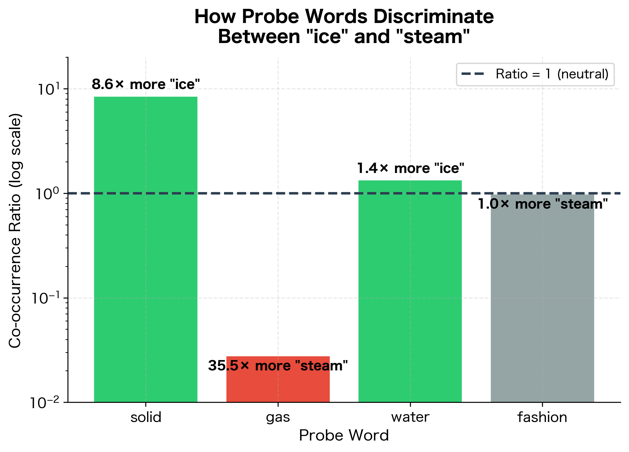
GloVe's key insight is simple but powerful: the ratio of co-occurrence probabilities encodes semantic relationships more reliably than raw probabilities. Consider the words "ice" and "steam." Both relate to water, but in different ways. How can we distinguish them?
Let's look at co-occurrence with probe words:
| Probe word | Ratio | ||
|---|---|---|---|
| solid | high | low | large (>> 1) |
| gas | low | high | small (<< 1) |
| water | high | high | ≈ 1 |
| fashion | low | low | ≈ 1 |
The raw probabilities and depend on many factors: how common each word is, the corpus domain, and so on. But the ratio tells a cleaner story:
- Large ratio: The probe word relates more to "ice" than "steam" (like "solid")
- Small ratio: The probe word relates more to "steam" than "ice" (like "gas")
- Ratio ≈ 1: The probe word relates equally to both (like "water") or to neither (like "fashion")
This ratio invariance is powerful. It factors out corpus-specific biases and isolates the semantic relationship we care about.
The ratios reveal clear discriminative patterns. "Solid" has a ratio far greater than 1 (approximately 8.6), indicating strong association with "ice" rather than "steam." Conversely, "gas" has a ratio well below 1 (approximately 0.03), showing the opposite relationship. Both "water" and "fashion" have ratios near 1, but for different reasons: "water" relates equally to both states, while "fashion" is irrelevant to either.
The ratio of co-occurrence probabilities encodes how a probe word discriminates between target words and . GloVe's objective function is designed so that word vectors can reconstruct these ratios.
From Ratios to Vectors: Deriving the Objective
We've established that co-occurrence ratios encode semantic relationships. The next question is: how do we design word vectors that naturally capture these ratios? The answer comes through a derivation that starts with a simple requirement and, through a series of logical constraints, arrives at GloVe's objective function.
The derivation unfolds like a detective story. Each constraint eliminates possibilities, narrowing the space of potential solutions until only one sensible answer remains. By the end, the objective function won't feel like an arbitrary choice. It will feel inevitable.
Setting Up the Problem
Our starting point is the co-occurrence matrix . This matrix is the foundation of everything GloVe does. Each entry counts how often word appears within a context window of word , accumulated across the entire corpus. From these raw counts, we can define probabilities:
where:
- : probability of word appearing in context of word
- : co-occurrence count for words and
- : total co-occurrence count for word
Now we can state our goal precisely. We want to learn word vectors and context vectors such that some function of these vectors recovers the co-occurrence ratio:
where:
- : word vectors for the target words
- : context vector for the probe word
- : function to be determined
This equation captures our key insight: the ratio of co-occurrence probabilities, the same ratio that distinguishes "ice" from "steam" via probe words like "solid" and "gas", should be computable from word vectors alone. The question is: what form must take?
Constraint 1: Vector Differences Encode Contrasts
The ratio fundamentally measures a contrast: how does word 's relationship with differ from word 's relationship with ? In vector spaces, the natural way to represent contrasts is through subtraction. When we compute , we obtain a vector pointing from toward , encoding everything that distinguishes them.
This suggests simplifying our function to depend on the difference:
Now takes two inputs: the difference vector and the context vector . This is already more constrained. doesn't need to handle three arbitrary vectors, just a difference and a context.
Constraint 2: Producing a Scalar from Vectors
Look at the right-hand side: is a scalar, a single number. But our inputs are vectors, high-dimensional objects with many components. How do we combine two vectors to produce a single number?
The most natural choice is the dot product. The dot product measures how aligned two vectors are: positive when they point similarly, negative when opposite, zero when perpendicular. It also has mathematical properties that will prove crucial shortly.
This gives us:
The function now operates on a scalar (the dot product) and produces another scalar. We've reduced the problem significantly.
Constraint 3: The Exponential Emerges
Here's where the key insight emerges. First, let's expand the dot product using the distributive property:
where:
- : dot product between word 's vector and context 's vector
- : dot product between word 's vector and context 's vector
The left side is a difference of dot products. But look at the right side of our original equation: is a ratio of probabilities. We need a function that transforms differences into ratios.
Step 1: Identify the required property. Think about this algebraically: we need such that for scalars and . This is asking for a homomorphism from addition to multiplication, a function that converts additive structure into multiplicative structure.
Step 2: Recognize the exponential as the solution. There's essentially one continuous function with this property: the exponential. The key identity is:
This works because . The exponential naturally converts differences in the exponent into ratios in the output.
Step 3: Apply the exponential. Substituting into our equation from Constraint 2, we get:
Step 4: Separate the terms. Using the exponential property , we can rewrite the left side:
Step 5: Match numerators and denominators. For this equality to hold for all word pairs and all probe words , the numerators must be proportional and the denominators must be proportional. This means each individual term must satisfy:
where:
- : exponential of the dot product between word and context vectors
- : probability of word appearing in context of word
- : a constant that may depend on but cancels when we take ratios
Step 6: Take logarithms. To make this more tractable, we take the natural logarithm of both sides:
This transforms the multiplicative relationship back into an additive one, which is easier to work with during optimization.
Arriving at the Core Equation
We're almost there. From Step 6 above, we have . Now we substitute the definition of the conditional probability :
Using the logarithm property :
where:
- : co-occurrence count for word and context word
- : total co-occurrence count for word across all contexts
- : the proportionality constant from Step 5 (may depend on )
Now notice something important: depends only on word , not on the context word . This term captures how often word appears in the corpus overall, a frequency effect rather than a semantic relationship. Similarly, might depend only on .
The solution is to absorb these word-specific terms into bias terms:
- Let
- Let
This yields GloVe's core equation:
where:
- : word vector for word (a -dimensional vector capturing semantic content)
- : context vector for word (a -dimensional vector capturing contextual role)
- : bias term for word (a scalar absorbing overall frequency effects)
- : bias term for context word (a scalar absorbing context-specific effects)
- : co-occurrence count (the observed data we're trying to predict)
This equation has a clear interpretation. The dot product measures the semantic compatibility between word and context . The biases adjust for how common each word is overall. Together, they should predict the logarithm of how often we actually observe the pair together.
This is GloVe's core equation: the dot product of word and context vectors, plus biases, should equal the log co-occurrence count.
The GloVe Objective Function
We've derived that word vectors should satisfy . But this is an idealized equation. In practice, no finite-dimensional embedding can perfectly satisfy it for every word pair. We need to frame this as an optimization problem: find the vectors and biases that come as close as possible to satisfying the equation across all pairs.
The journey from ideal equation to practical objective reveals important design decisions. A naive formulation encounters serious problems, and solving them leads to GloVe's distinctive weighted least squares approach.
Naive Least Squares (and Its Problems)
The most straightforward optimization minimizes squared error:
where:
- : the objective function (total loss) to minimize
- : our model's prediction for word pair
- : the target log co-occurrence count
- The sum is over all word pairs in the vocabulary
This says: for every word pair, measure how far our prediction deviates from the target log co-occurrence, square it (so positive and negative errors contribute equally), and sum across all pairs. Standard least squares.
But this formulation has critical flaws:
-
Zero counts are catastrophic: Many word pairs never co-occur in any corpus. "Quantum" and "umbrella" might never appear together. For these pairs, , and . The objective becomes undefined.
-
Not all pairs deserve equal attention: A co-occurrence count of 1 million reflects a strong, statistically reliable signal. A count of 1 might be noise, a single accidental co-occurrence. Yet naive least squares weights them identically.
-
Rare pairs can dominate: If rare word pairs have large errors (which they often do, being noisy), they can disproportionately influence training, pulling embeddings away from configurations that would serve common words well.
These problems demand a more thoughtful objective.
The Weighting Function
GloVe's solution is to introduce a weighting function that modulates how much each word pair contributes to the objective. This function is designed to satisfy three requirements:
-
Zero weight for zero counts: When , set . This pair simply doesn't contribute. We never try to predict .
-
Increasing weight with frequency: Pairs that co-occur more often provide more reliable statistics. The function should increase with , giving more weight to confident observations.
-
Bounded influence: Extremely common word pairs (like "the" with almost everything) shouldn't completely dominate training. The weight should eventually plateau.
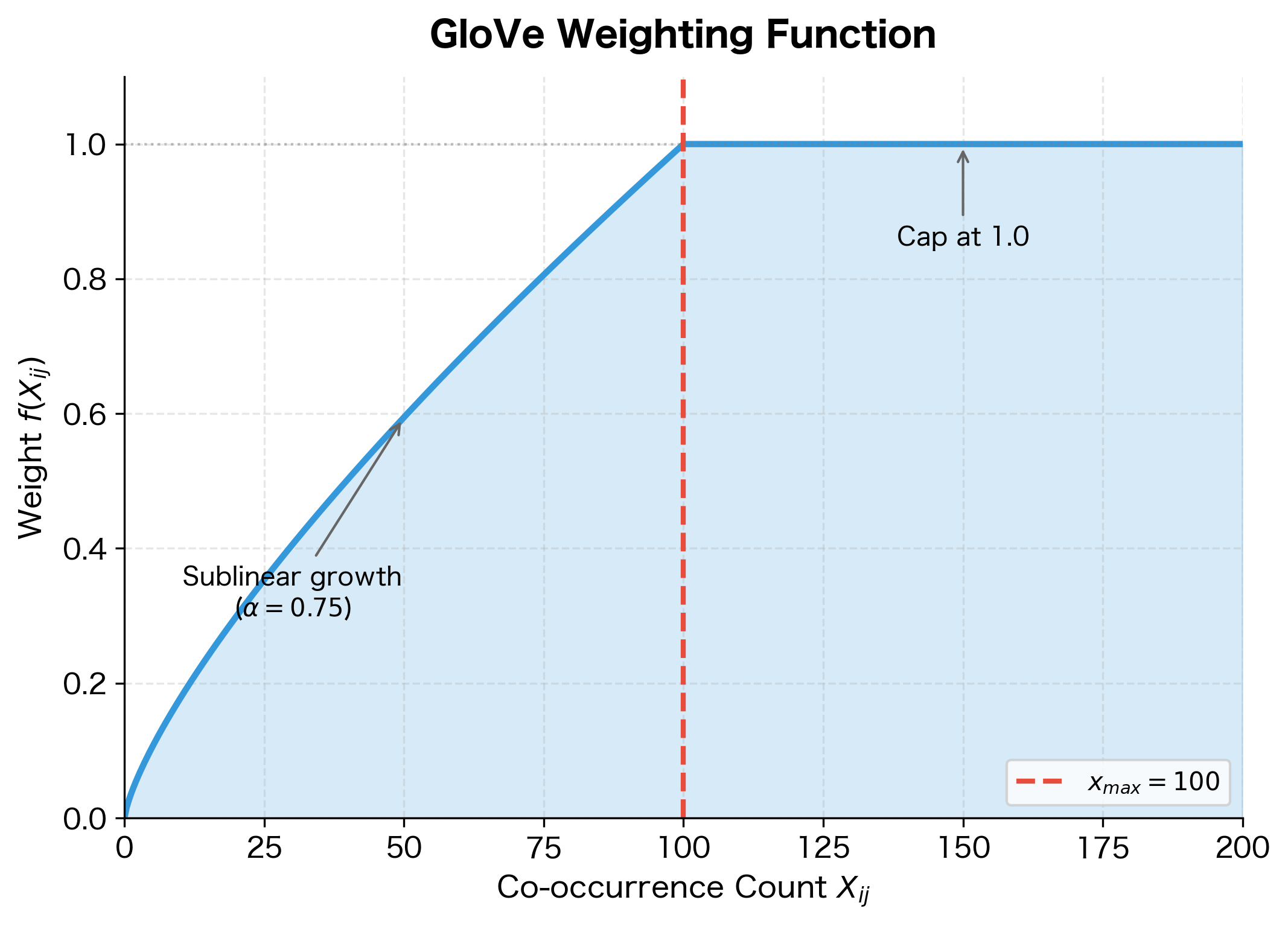
The function that GloVe adopts balances these requirements:
where:
- : co-occurrence count for a particular word pair
- : cutoff parameter (typically 100), beyond which the weight saturates
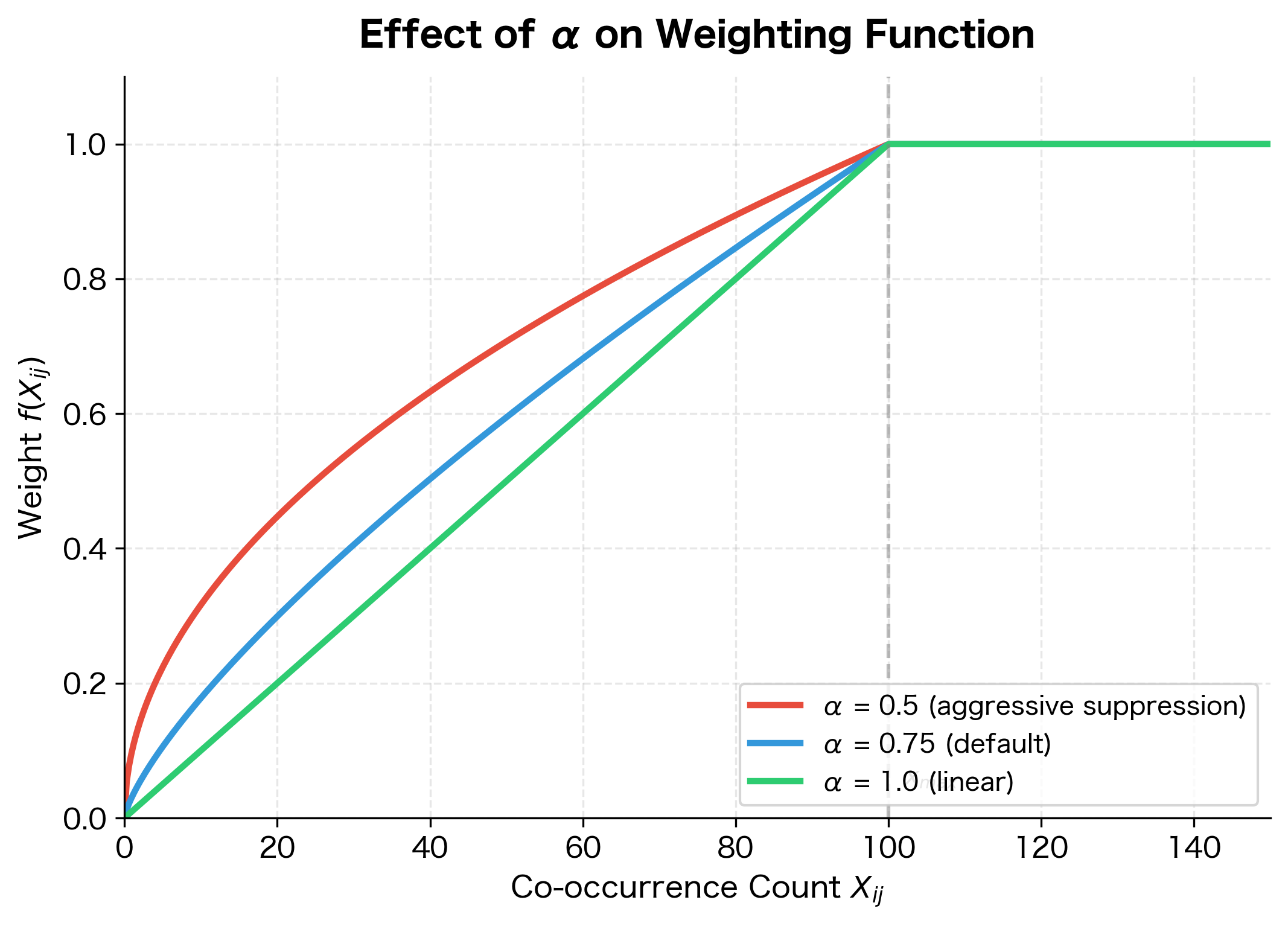
- : exponent (typically 0.75), controlling how quickly weight grows with frequency
Why this form works. The function has two regimes:
-
Below the cutoff (): The weight grows sublinearly with co-occurrence count. The exponent (less than 1) ensures that doubling the count doesn't double the weight. Instead, it increases by a factor of . This dampens the influence of very frequent pairs while still giving them more weight than rare pairs.
-
At or above the cutoff (): The weight caps at 1.0. This prevents the most frequent word pairs (like "the" with common words) from completely dominating the training signal.
The weighting shows clear progression: a count of 1 receives weight 0.18, while a count of 50 gets 0.65. Once the count reaches 100 (the x_max threshold), the weight caps at 1.0 and stays there for higher counts. This sublinear scaling () means common word pairs contribute meaningfully to training without completely dominating rare but informative pairs.
The Complete Objective
Combining the core equation with the weighting function:
where:
- : objective function to minimize
- : vocabulary size
- : weighting function for word pair
- : word vector for word
- : context vector for word
- : bias terms
- : co-occurrence count
This is a weighted least squares problem: find vectors and biases that minimize the weighted squared error between predicted and actual log co-occurrences.
GloVe minimizes weighted squared error between and , where the weight increases with co-occurrence frequency up to a maximum. The sum runs only over pairs with .
Building the Co-occurrence Matrix
Before training GloVe, we must construct the co-occurrence matrix from a corpus. This preprocessing step represents a fundamental difference from Word2Vec: while Word2Vec processes training pairs on-the-fly during optimization, GloVe separates statistics gathering from model training. We scan the corpus once to build the co-occurrence matrix, then train on these precomputed counts.
This separation has important implications. The matrix construction phase is embarrassingly parallel, since each document can be processed independently. Once complete, the training phase operates on a fixed set of statistics, making it more predictable and easier to tune. The tradeoff is memory: we must store the entire matrix (though sparse representations help enormously).
Defining Co-occurrence
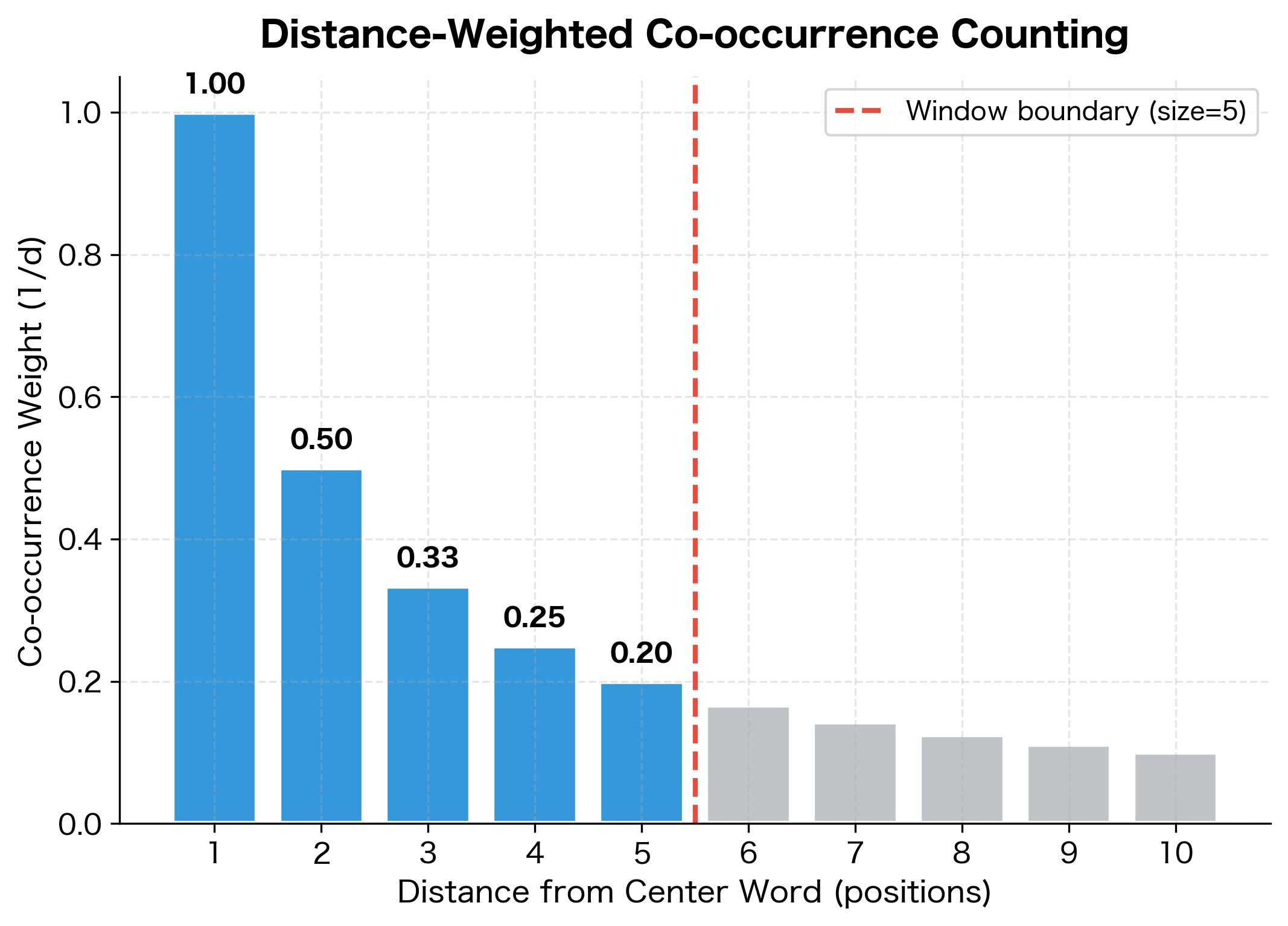
The core question is: what exactly should we count? A word pair "co-occurs" when word appears within a context window of word . But not all co-occurrences are equal. GloVe uses distance-weighted counting, where closer words contribute more to the co-occurrence count than distant ones.
The rationale is linguistic: words immediately adjacent typically have stronger relationships than words at the edges of a context window. In the phrase "the quick brown fox," "quick" and "brown" are more closely related than "the" and "fox," even though both pairs fall within a five-word window.
Specifically, if words and are separated by positions, we add to :
where:
- : the distance in positions between words and (1 for adjacent words, 2 for one word apart, etc.)
- : the co-occurrence count being accumulated
Adjacent words (distance 1) contribute a full count of 1.0. Words two positions apart contribute 0.5. At the edge of a window of size 5, the contribution is just 0.2. This inverse-distance weighting encodes the intuition that proximity correlates with semantic relevance.
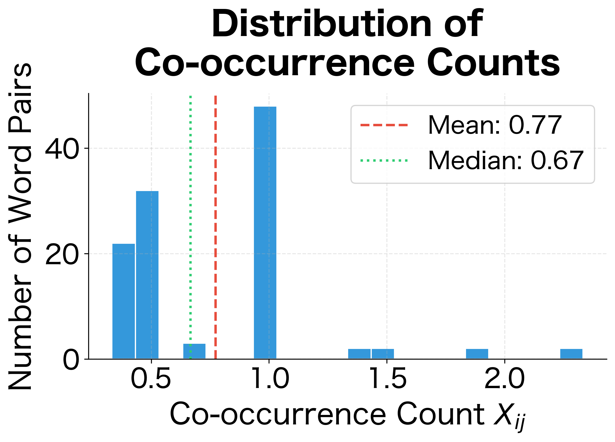
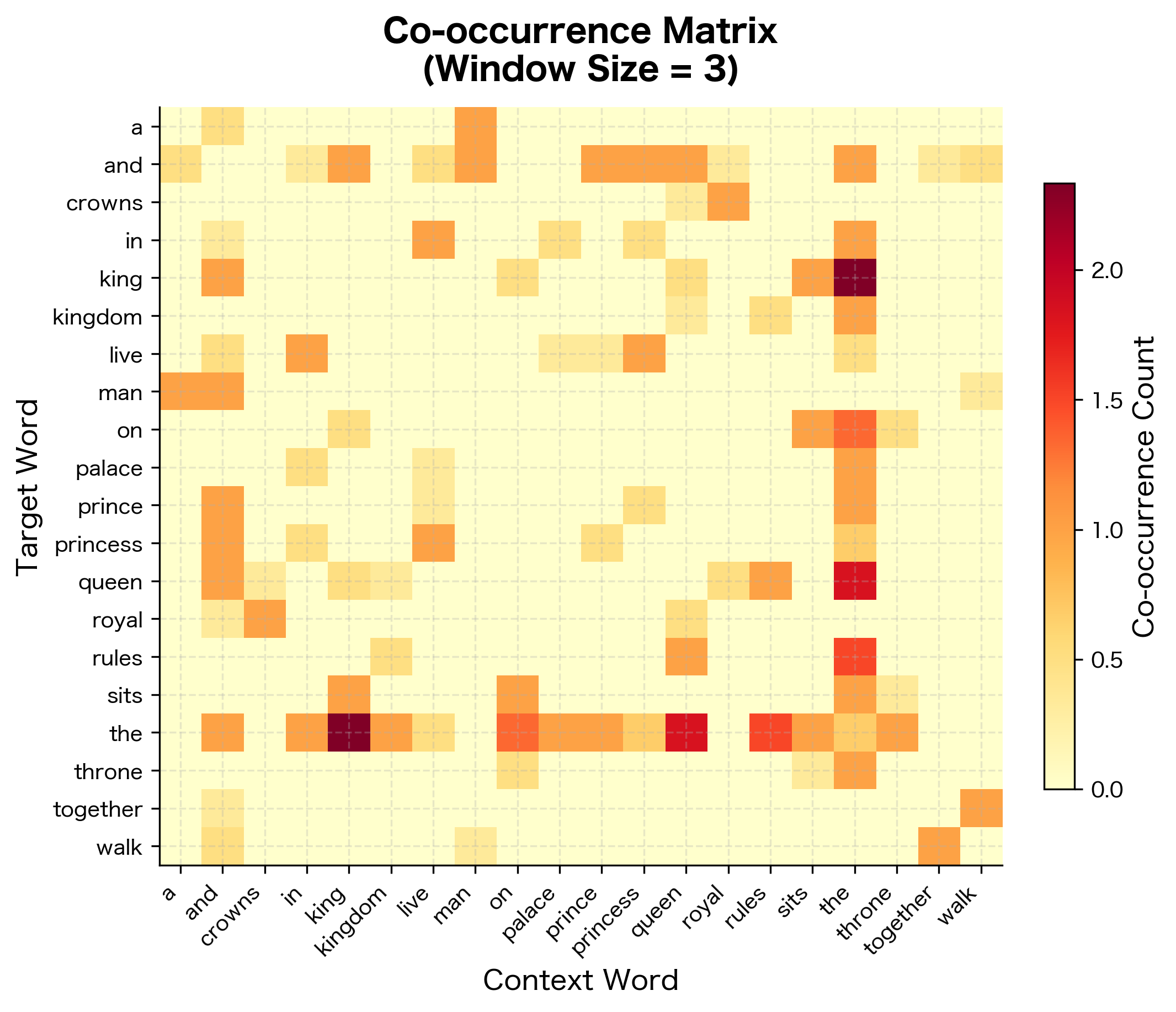
The matrix shows typical characteristics of word co-occurrence data. Even with this tiny corpus, the sparsity is substantial, as most word pairs never appear together within a context window. The highest co-occurrence counts involve "the," which appears frequently throughout the corpus. The distance-weighted counting produces fractional values: a count of 1.50 indicates two co-occurrences at different distances (e.g., adjacent words contribute 1.0, while words two positions apart contribute 0.5).
Symmetry and Sparse Storage
The co-occurrence matrix is nearly symmetric: . For undirected context windows (looking both left and right), it's exactly symmetric. In practice, we often symmetrize the matrix by averaging:
where:
- : the symmetrized co-occurrence count
- : count of word appearing in context of word
- : count of word appearing in context of word
This symmetrization ensures that the relationship between words and is treated the same regardless of which word is considered the "center" word.
For large vocabularies, the co-occurrence matrix is extremely sparse. A 100,000-word vocabulary produces a 10-billion-entry matrix, but most entries are zero. Efficient implementations use sparse matrix formats, storing only non-zero entries.
For this small vocabulary, the sparse format provides modest savings. The real benefit emerges at scale: a 100,000-word vocabulary would require approximately 80 GB for a dense matrix (100,000² × 8 bytes), while the sparse representation stores only non-zero entries, typically a few hundred megabytes. This difference makes large-scale GloVe training feasible on commodity hardware.
Relationship to Matrix Factorization
Stepping back from the implementation details reveals a deeper perspective on what GloVe is doing. The objective function we derived places GloVe squarely in the family of matrix factorization methods, the same family that includes techniques like Singular Value Decomposition (SVD) and Latent Semantic Analysis (LSA). Understanding this connection illuminates both why GloVe works and how it relates to classical dimensionality reduction.
Consider the equation we derived:
This equation holds for every word pair . If we stack all word vectors into a matrix and all context vectors into a matrix , we can write this as a matrix equation.
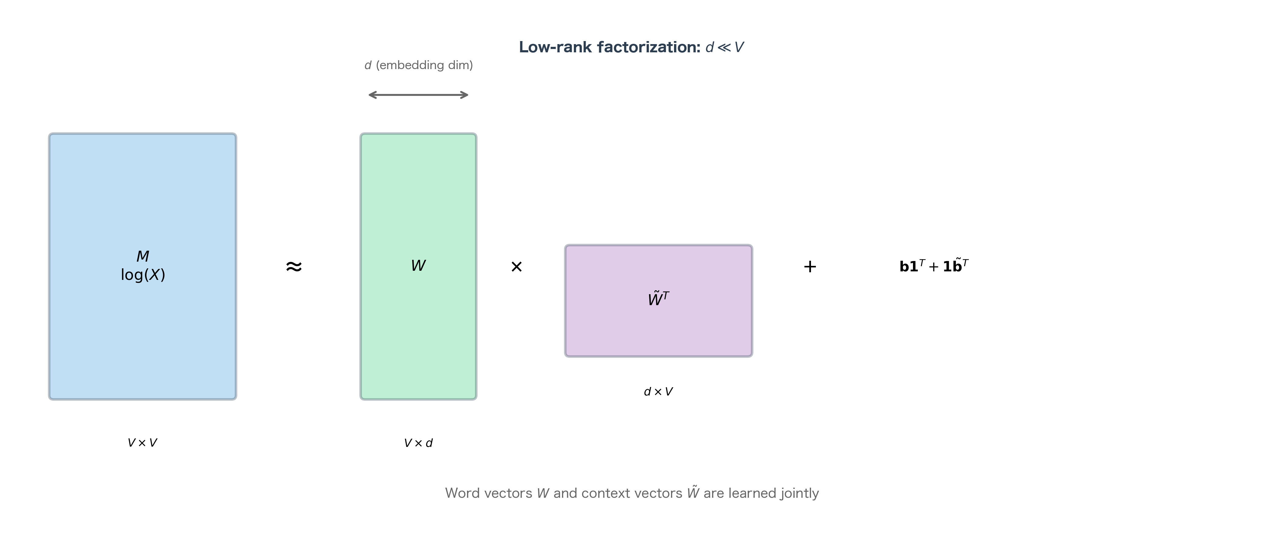
Let's define a target matrix where each entry for non-zero co-occurrences. Then GloVe approximately factorizes this log-count matrix:
where:
- : log co-occurrence matrix of size , where
- : matrix of word vectors of size , where row is
- : matrix of context vectors of size , where row is
- : the matrix product, where entry equals
- : column vector of word biases of size
- : column vector of context biases of size
- : column vector of ones of size
- : outer product creating a matrix where row has all entries equal to
- : outer product creating a matrix where column has all entries equal to
This is a form of weighted, biased matrix factorization. The key insight is dimensional: the original matrix is , potentially enormous for large vocabularies. The factorization represents it as the product of much smaller matrices: and are both , where (typically 50-300) is vastly smaller than (potentially hundreds of thousands).
This compression is exactly what we want. The low-rank structure forces the model to discover patterns. It can't store the full matrix, so it must learn generalizable representations that explain many co-occurrences with few parameters. The resulting vectors capture the essential semantic content of words, distilled from millions of co-occurrence observations.
The weighting function makes this a weighted factorization, prioritizing accurate reconstruction of reliable observations. The biases make it biased (in the technical sense), allowing frequency effects to be absorbed separately from semantic content.
Connection to Classical Methods
This matrix factorization perspective connects GloVe to classical methods like Latent Semantic Analysis (LSA), which factorizes term-document matrices using Singular Value Decomposition (SVD). Key differences:
| Aspect | LSA (SVD) | GloVe |
|---|---|---|
| Matrix | Term-document | Word-word co-occurrence |
| Transform | Raw counts or TF-IDF | Log counts |
| Weighting | Uniform | Frequency-based |
| Optimization | Exact SVD | Stochastic gradient descent |
| Biases | None | Word and context biases |
GloVe inherits the global perspective of matrix factorization while adding neural-network-style training flexibility.
Training GloVe
With the objective function and co-occurrence matrix defined, we can train GloVe using stochastic gradient descent. Unlike neural networks with complex layer compositions, GloVe's gradient computation is straightforward. The objective is a simple weighted sum of squared errors, and each term depends on only four parameters (two vectors and two biases).
The training process iterates through non-zero entries of the co-occurrence matrix, computing gradients and updating parameters. Because each word pair's contribution is independent, the computation parallelizes naturally across CPU cores or GPU threads.
Gradient Derivation
Understanding the gradients illuminates how learning proceeds. For a single word pair with co-occurrence count , the contribution to the objective is:
where:
- : loss contribution from word pair
- : weighting function that prioritizes frequent co-occurrences
- : our model's prediction
- : the target value we want to predict
To derive the gradients, let's introduce cleaner notation that separates the prediction, target, and error:
- (the model's prediction)
- (the target value)
- (the prediction error)
The objective for this pair becomes . This is a weighted squared error: we penalize the squared prediction error, but modulate the penalty by the weight .
Step 1: Apply the chain rule. To find the gradient with respect to any parameter , we use the chain rule. Since and is a constant (it depends on the data, not the parameters):
Since and is a constant, we have :
Step 2: Compute partial derivatives of the prediction. Since , we can compute how the prediction changes with each parameter:
- (the derivative of with respect to is )
- (the derivative of with respect to is )
- (the derivative of with respect to itself is 1)
- (the derivative of with respect to itself is 1)
Step 3: Substitute to get the complete gradients. Plugging these partial derivatives into our chain rule formula:
Interpreting the gradients. Notice the symmetry: the gradient for word vectors involves the context vectors, and vice versa. This makes intuitive sense. To improve the prediction for the pair , we adjust in the direction of (or opposite, if we're overshooting the target). The magnitude of the adjustment depends on:
- The error : larger errors lead to larger updates
- The weight : frequent co-occurrences receive larger updates
The biases have particularly simple gradients: just the weighted error, with no vector component. They act as global adjustments, shifting predictions up or down for all contexts involving word or context .
Training Loop
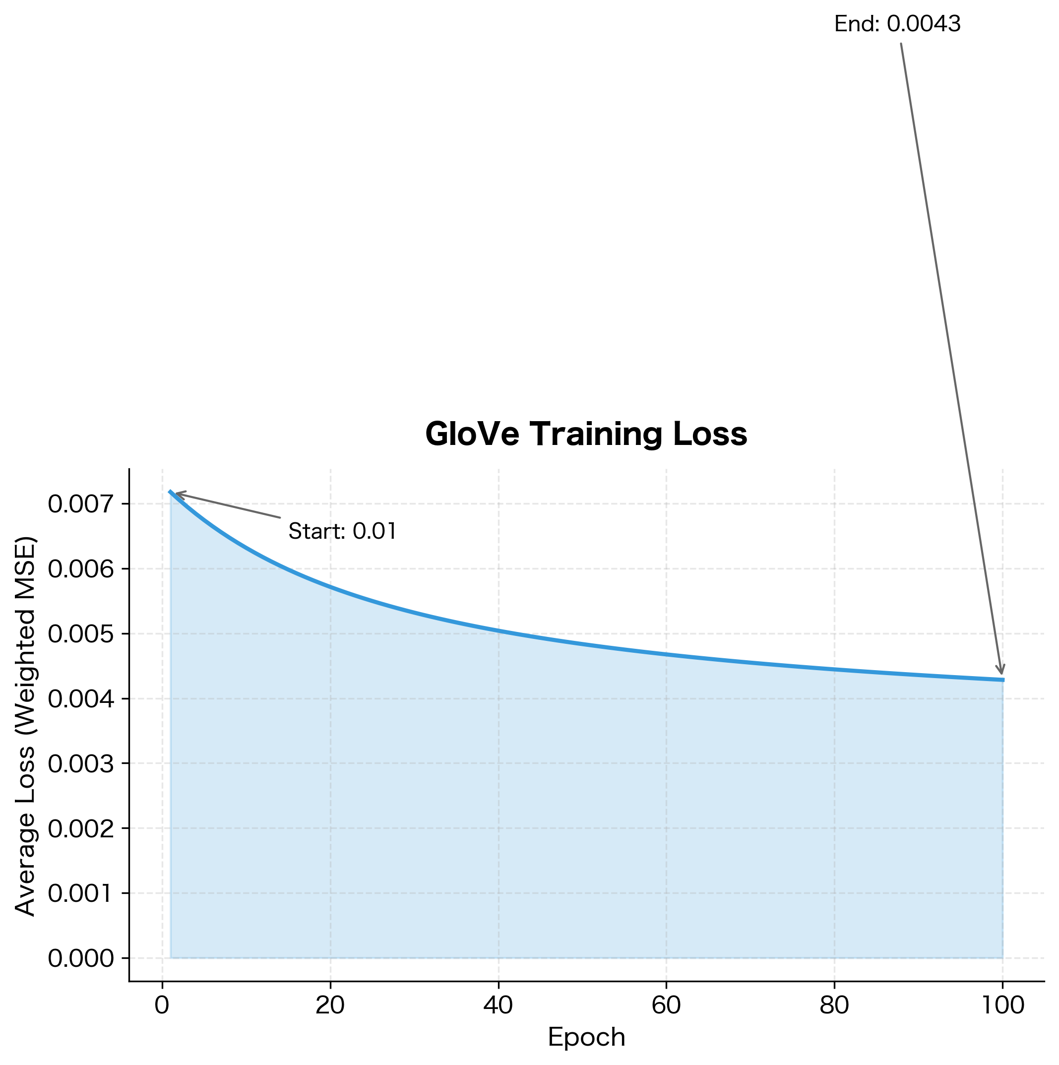
Training iterates over all non-zero co-occurrence pairs, updating embeddings using gradient descent. The original GloVe implementation uses AdaGrad, an adaptive learning rate method that helps with the highly varying frequencies of word pairs.
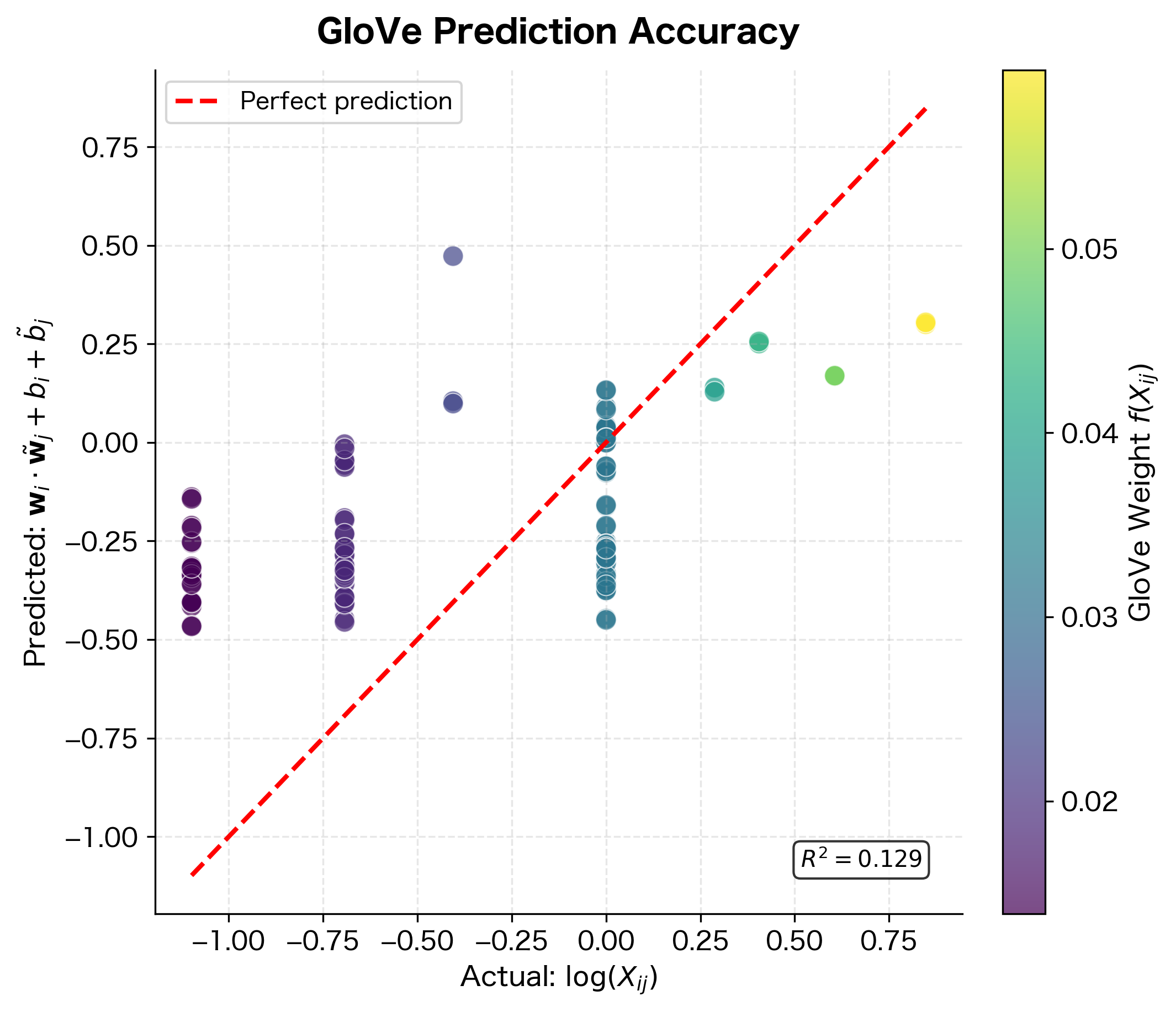
The substantial loss reduction indicates the model successfully learned to predict log co-occurrence counts. The weighted least squares objective prioritizes high-frequency pairs, so the final embeddings should capture the dominant co-occurrence patterns in the corpus. The remaining loss reflects both inherent noise in co-occurrence statistics and the capacity limitations of a 20-dimensional embedding space.
The Role of Bias Terms
GloVe includes bias terms and in its objective. These aren't just mathematical conveniences; they play a crucial role in capturing word frequency effects.
What Biases Capture
Consider a very frequent word like "the." It co-occurs with nearly every word in the vocabulary, leading to high co-occurrence counts across the board. Without biases, the model would try to explain these high counts through the embedding: "the" would need a large vector that has high dot product with everything.
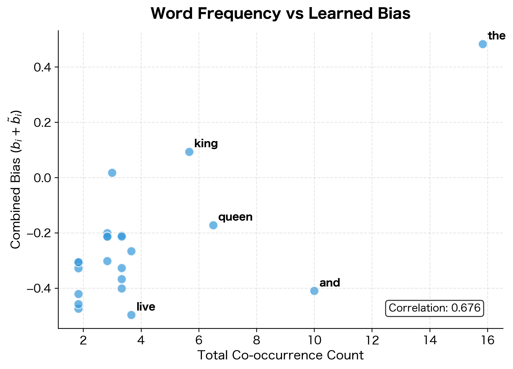
Biases absorb this frequency effect. The bias captures "how often word tends to co-occur in general." A word like "the" has a high bias, explaining its high co-occurrence counts without distorting its embedding.
The pattern is clear: words with higher total co-occurrence counts tend to have larger learned biases. The most frequent word in the corpus shows the highest combined bias, absorbing its tendency to co-occur with many different words. This prevents the embedding vectors from needing unnaturally large magnitudes to explain high co-occurrence counts, keeping the learned semantic relationships clean and interpretable.
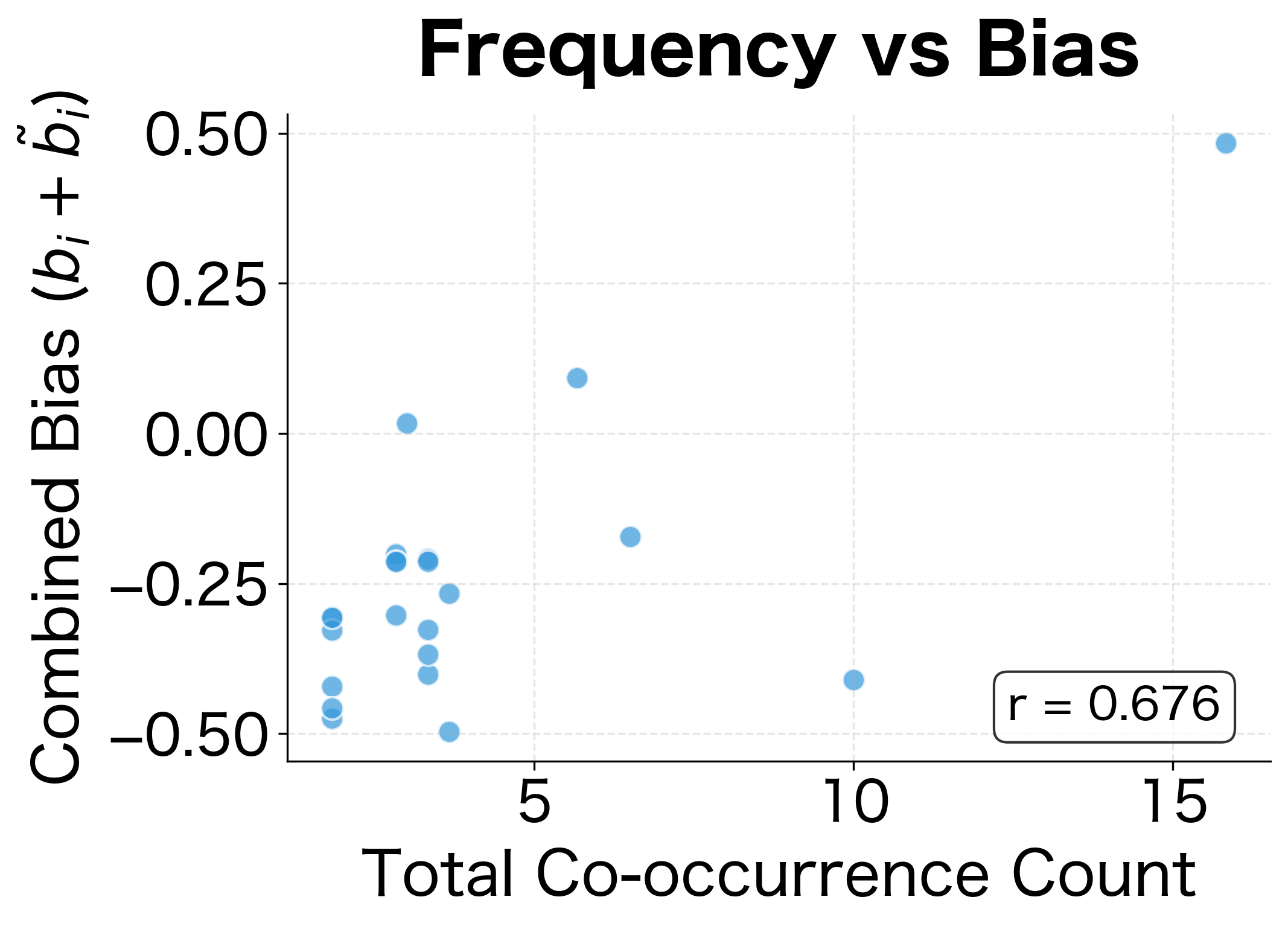
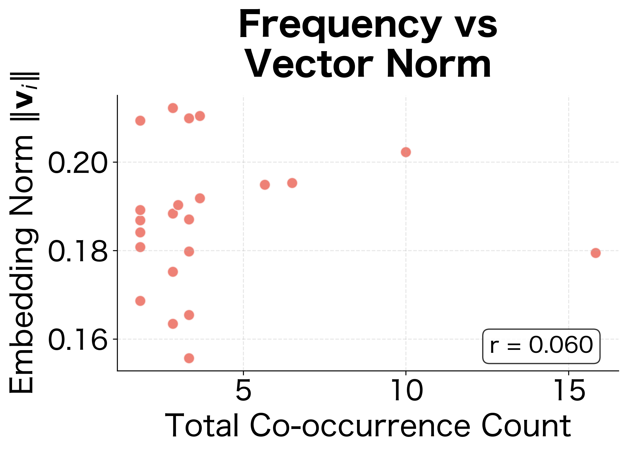
The comparison is striking. Biases show strong correlation with frequency (left panel), while embedding norms show weaker correlation (right panel). This confirms that biases are doing their job: absorbing frequency effects so that the embedding vectors can focus on encoding semantic content.
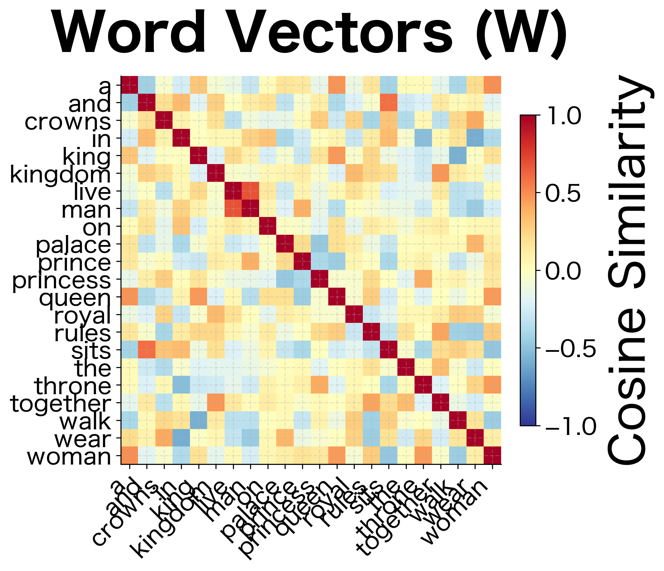
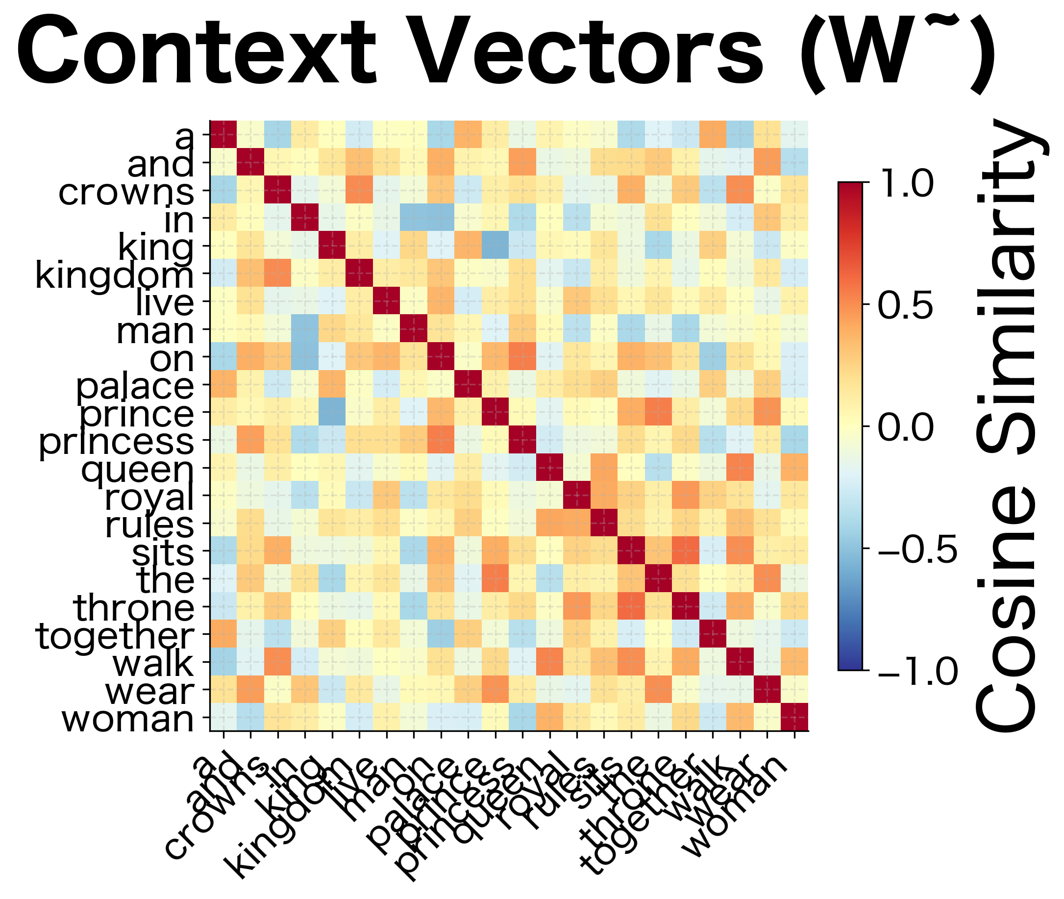
Combining Word and Context Vectors
GloVe learns two sets of vectors: word embeddings and context embeddings . Unlike Word2Vec, where these play asymmetric roles (center vs. context), GloVe's objective is symmetric in and . This symmetry means and carry similar information. Both encode how word relates to other words.
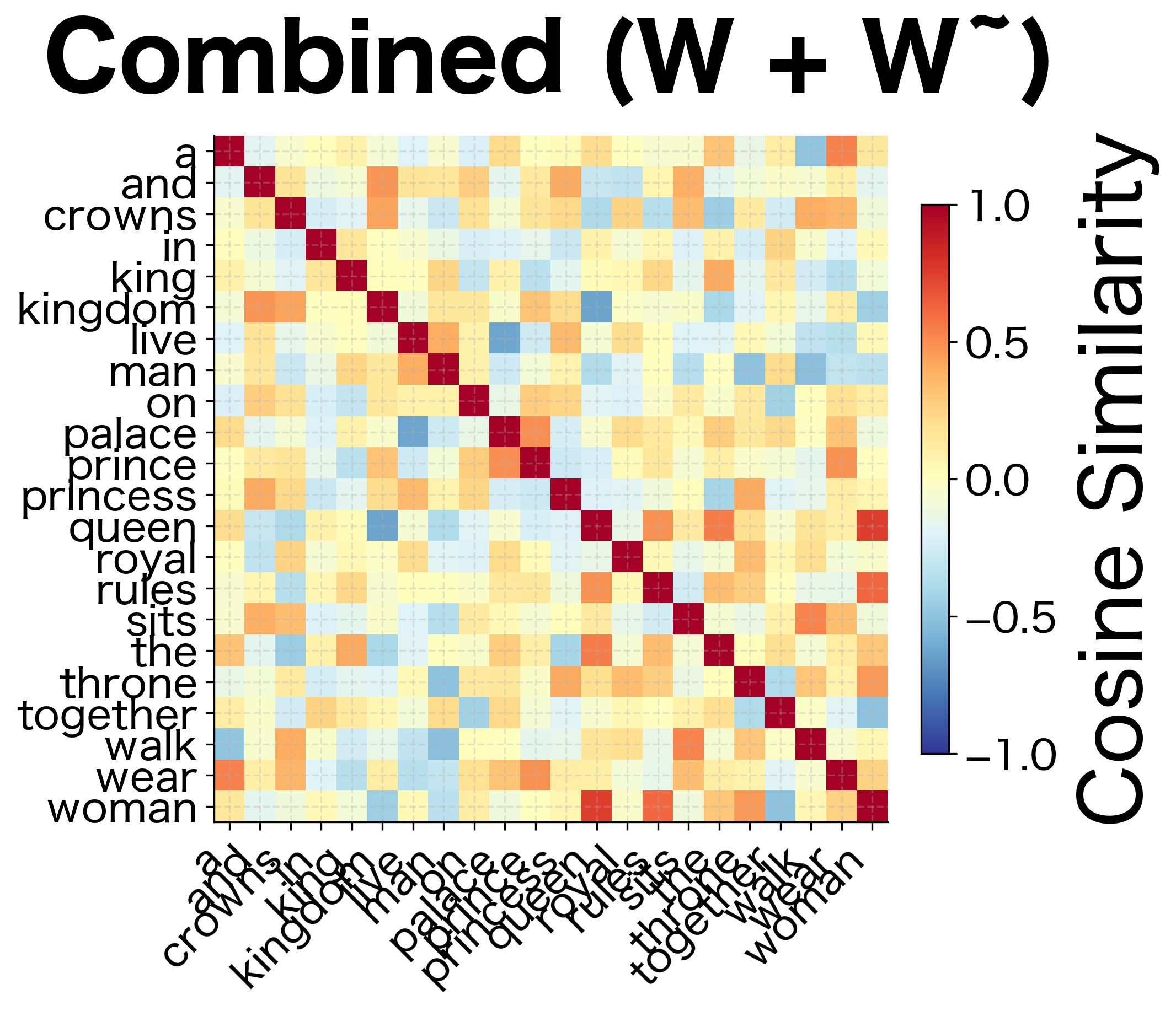
The original GloVe paper recommends combining them by simple addition:
where:
- : final word vector for word (the embedding used in downstream tasks)
- : word embedding from the word matrix (learned as the "center" representation)
- : context embedding from the context matrix (learned as the "context" representation)
This combination often produces better embeddings than either matrix alone. The intuition is twofold:
-
Noise reduction: Random initialization and stochastic training introduce noise into both and . Adding them tends to cancel out uncorrelated noise while reinforcing the true signal.
-
Complementary information: Although symmetric in theory, in practice the word and context vectors may capture slightly different aspects of word meaning. Combining them creates a richer representation.
GloVe vs Word2Vec: Key Differences
GloVe and Word2Vec both produce high-quality word embeddings, but they take fundamentally different approaches. Understanding these differences helps you choose the right method for your application.
Training Paradigm
| Aspect | Word2Vec (Skip-gram) | GloVe |
|---|---|---|
| Approach | Predictive (neural network) | Count-based (matrix factorization) |
| Input | Local context windows, one pair at a time | Global co-occurrence matrix |
| Objective | Predict context words from center word | Reconstruct log co-occurrence counts |
| Training | Online (streaming, can process infinite data) | Batch (requires full matrix upfront) |
Practical Considerations
Memory usage: GloVe requires storing the co-occurrence matrix (sparse but potentially large), while Word2Vec can stream data from disk.
Training speed: GloVe often converges faster because it uses global statistics. Word2Vec may need multiple passes over the corpus.
Parallelization: GloVe's matrix operations parallelize naturally on GPUs. Word2Vec's sequential updates are harder to parallelize, though implementations use negative sampling tricks.
Rare words: Both struggle with rare words, but GloVe's explicit co-occurrence counts make the signal clearer.
Empirical Performance
The original GloVe paper reported competitive results on word analogy and similarity tasks:
The GloVe paper showed substantial improvements over Word2Vec on these benchmarks, particularly for semantic analogies. However, subsequent research has demonstrated that careful hyperparameter tuning can close much of this gap. The choice between GloVe and Word2Vec often depends on practical considerations like data availability, memory constraints, and training infrastructure, rather than absolute quality differences.
Training GloVe Efficiently
Real-world GloVe training involves millions of words and billions of co-occurrences. Several techniques make this feasible.
Sparse Storage and Iteration
The co-occurrence matrix is extremely sparse. A 100,000-word vocabulary has 10 billion potential entries, but only millions are non-zero. Efficient training iterates only over non-zero entries.
AdaGrad Optimization
GloVe uses AdaGrad (Adaptive Gradient), which adapts the learning rate for each parameter based on its historical gradients. The intuition is simple: parameters that have been updated frequently (like biases for common words) should receive smaller updates to avoid overshooting, while parameters that have been updated rarely should receive larger updates to make faster progress.
The update rule at each time step is:
where:
- : the parameter value at time step (could be any component of , , , or )
- : the updated parameter value
- : base learning rate (typically 0.05 for GloVe)
- : current gradient at time
- : sum of squared gradients from all previous time steps
- : small constant (typically ) for numerical stability to avoid division by zero
The key insight is that the effective learning rate decreases as more updates accumulate. For frequently updated parameters, grows large, shrinking the effective learning rate. For rarely updated parameters, stays small, keeping the effective learning rate close to .
Parallelization
Each co-occurrence pair can be processed independently (up to synchronization of embedding updates). GPU implementations parallelize across thousands of pairs simultaneously.
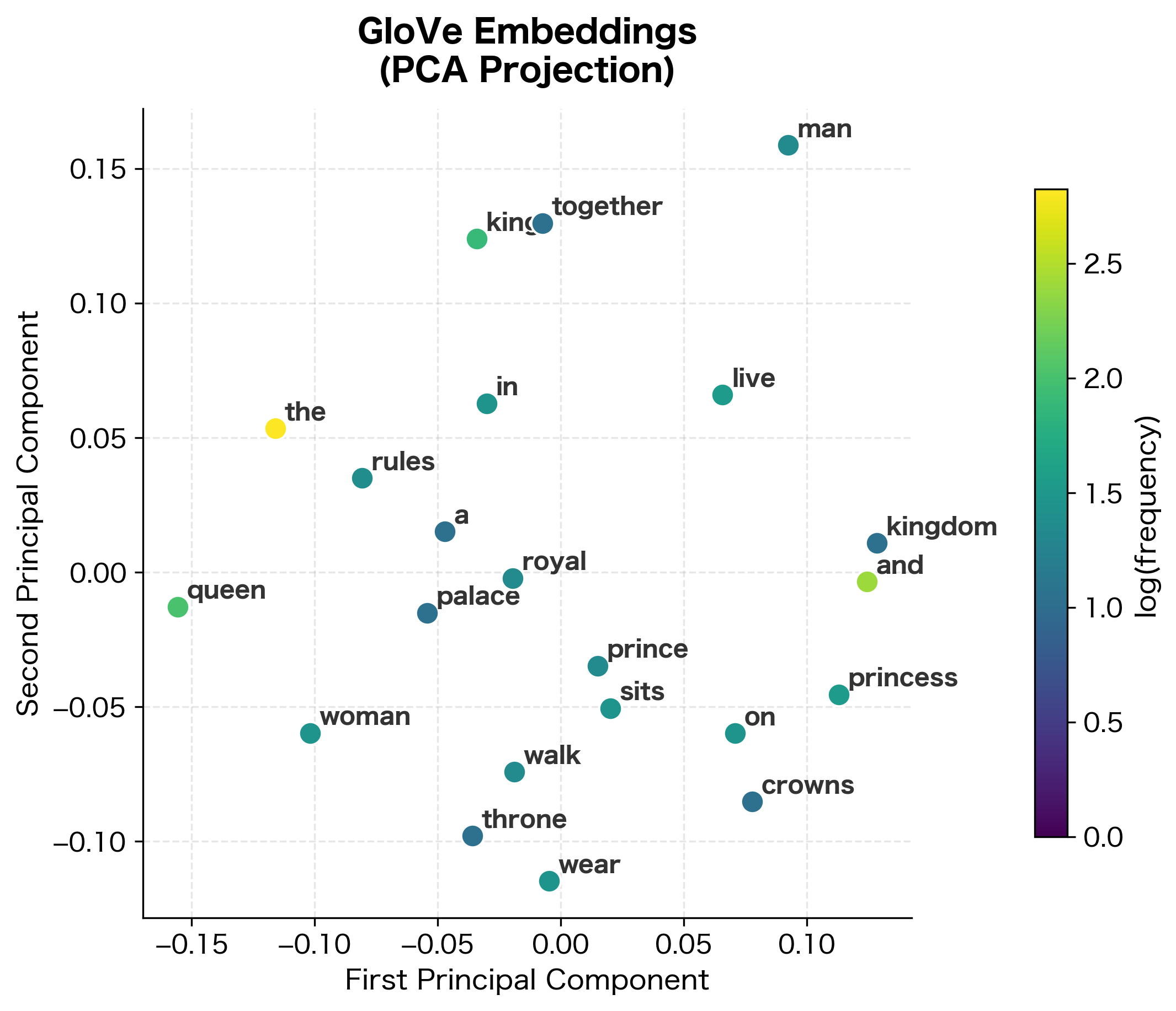
Evaluating GloVe Embeddings
Let's examine what our trained GloVe model has learned by looking at word similarities and the embedding structure.
With only five short sentences, the learned similarities reflect the limited corpus structure rather than general semantic knowledge. Words that frequently co-occur together show higher similarity scores. For larger corpora, GloVe embeddings would capture broader semantic relationships. "King" would be similar to "queen" because both appear in similar royal contexts across thousands of documents, not just in a handful of training sentences.
Practical Training with Larger Data
Our implementation works for small vocabularies, but real applications require optimization. Production GloVe training differs in several key ways:
- Memory-mapped files: Large co-occurrence matrices don't fit in memory. Production implementations use memory-mapped files or distributed storage.
- Shuffled iteration: To ensure stable training, iterations over co-occurrence pairs should be shuffled. This prevents the model from seeing all pairs involving "the" consecutively.
- Early stopping: Monitor the loss on a held-out portion of the co-occurrence matrix. Stop when validation loss stops improving.
- Vector dimension: Typical dimensions range from 50-300. Larger dimensions capture more nuance but require more data and compute.
The choice of embedding dimension involves a bias-variance tradeoff. Lower dimensions force the model to compress information, which can provide regularization but may miss subtle distinctions. Higher dimensions allow more expressive representations but require more training data to avoid overfitting and more memory for storage and computation.
Limitations and Considerations
GloVe produces high-quality embeddings but has limitations worth understanding:
- Static embeddings: Like Word2Vec, GloVe produces one vector per word regardless of context. "Bank" has the same embedding whether referring to a financial institution or a river bank.
- Out-of-vocabulary words: GloVe cannot generate embeddings for words not in the training vocabulary. Unlike subword methods (FastText), it has no mechanism for morphological generalization.
- Window size sensitivity: The choice of context window affects which co-occurrences are captured. Larger windows capture more topical similarity; smaller windows capture syntactic patterns.
- Memory requirements: The co-occurrence matrix, while sparse, can be large. A 400,000-word vocabulary might produce a matrix with billions of non-zero entries.
- Corpus bias: Embeddings reflect biases in the training corpus. Associations between professions and genders, for example, are encoded in the vectors.
Summary
GloVe approaches word embeddings from a different angle than Word2Vec. By explicitly factorizing the log co-occurrence matrix with carefully designed weighting, it produces embeddings that encode both local and global corpus statistics.
Key takeaways:
-
Co-occurrence ratios encode meaning: The ratio reveals how a probe word discriminates between targets. GloVe's objective makes word vectors reconstruct these ratios.
-
Weighted least squares: The objective minimizes weighted squared error between and , with weights that prioritize frequent co-occurrences.
-
Matrix factorization perspective: GloVe factorizes the log co-occurrence matrix into word and context embeddings plus biases. This connects it to classical methods like LSA.
-
Bias terms absorb frequency: Word and context biases capture overall frequency effects, preventing common words from distorting the embedding geometry.
-
Combined vectors work best: The final embedding is typically , averaging the word and context vectors learned during training.
-
Competitive with Word2Vec: Despite the different approach, GloVe achieves comparable results on standard benchmarks, with trade-offs in memory usage and training paradigm.
The next chapter explores FastText, which extends Word2Vec with subword information, enabling the model to handle morphologically rich languages and out-of-vocabulary words.
Key Parameters
When training GloVe models, several hyperparameters affect the quality of learned embeddings:
embedding_dim (typical range: 50-300): The dimensionality of word vectors.
- Lower values (50-100): Faster training, smaller memory footprint. Good for similarity tasks.
- Higher values (200-300): Captures more nuanced relationships. Better for downstream tasks and analogy completion.
- Common choice: 100-200 for most applications; 300 for benchmarks.
window_size (typical range: 5-15): Context window for building the co-occurrence matrix.
- Smaller windows (5-8): Emphasize syntactic relationships.
- Larger windows (10-15): Capture broader semantic/topical similarity.
- Common choice: 10-15 for semantic tasks.
x_max (typical value: 100): Cutoff for the weighting function.
- Co-occurrences above this threshold receive weight 1.0.
- Lower values give more uniform weighting; higher values let frequent pairs dominate more.
- Common choice: 100 (from the original paper).
alpha (typical value: 0.75): Exponent in the weighting function.
- Controls how quickly weight increases with co-occurrence count.
- Lower values (0.5) more aggressively dampen frequent pairs.
- Higher values (1.0) approach raw-count weighting.
- Common choice: 0.75 (from the original paper).
min_count (typical range: 1-100): Minimum word frequency to include in vocabulary.
- Lower values include rare words but may produce noisy embeddings.
- Higher values produce more robust embeddings but exclude rare words.
- Common choice: 5-10 for large corpora.
learning_rate (typical value: 0.05): Initial learning rate for AdaGrad.
- Higher values speed training but may overshoot.
- AdaGrad adapts rates per-parameter, so the initial value is less critical than with SGD.
- Common choice: 0.05.
epochs (typical range: 25-100): Number of passes through the co-occurrence data.
- Fewer epochs for very large matrices.
- More epochs for smaller datasets or when loss hasn't converged.
- Common choice: 50-100.
Quiz
Ready to test your understanding? Take this quick quiz to reinforce what you've learned about GloVe word embeddings.

Comments