Negative Sampling: Efficient Word Embedding Training

Negative SamplingLink Copied

The Skip-gram model learns powerful word representations, but it has a computational Achilles' heel: the softmax denominator. Every training step requires computing a sum over the entire vocabulary:

where:

• $P(w_c | w_t)$: probability of context word $w_c$ given center word $w_t$
• $\mathbf{w}'_c$: context embedding vector for word $w_c$
• $\mathbf{w}_t$: center embedding vector for word $w_t$
• $V$: vocabulary size

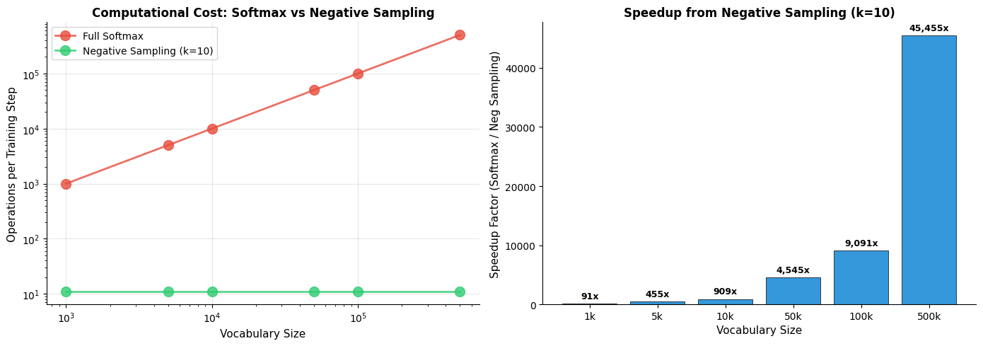
For a vocabulary of 100,000 words, this means 100,000 dot products and exponentials per training step. With billions of training examples, full softmax becomes impractical. Training would take months instead of days.

Negative sampling solves this problem differently: instead of predicting the exact probability of a context word, we reformulate the task as binary classification. Given a word pair, is it a genuine context pair from the corpus, or a fake pair we constructed? This transformation reduces the computational cost from $O(V)$ to $O(k)$, where $k$ is a small constant (typically 5-20), making large-scale training feasible.

This chapter develops negative sampling from first principles. We'll derive the objective function, understand why the clever sampling distribution matters, implement efficient training, and see how this approximation achieves nearly the same quality as full softmax at a fraction of the cost.

The Core Insight: Binary Classification Instead of SoftmaxLink Copied

The full Skip-gram model tries to answer: "What is the probability of each vocabulary word being a context word?" This requires computing a probability distribution over 100,000+ words.

Negative sampling asks a simpler question: "Is this specific word pair a real context pair or a fake one?" This is binary classification, requiring only a single probability per pair.

Consider the sentence "The quick brown fox jumps." When "fox" is the center word, "brown" is a genuine context word. But what about "elephant" or "democracy"? These words don't appear near "fox" in this context. They're negatives, and we can use them to train the model.

The model learns by trying to maximize the probability for the positive pair and minimize it for the negative pairs. Through millions of such updates, the embedding space organizes so that words appearing in similar contexts end up nearby.

From Softmax to SigmoidLink Copied

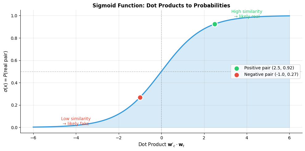
The mathematical reformulation is straightforward. Instead of softmax, we use the sigmoid function $\sigma(x) = 1 / (1 + e^{-x})$ to output a probability for each pair independently.

For a positive (center, context) pair, we want:

where:

• $D = 1$: indicator that the pair came from the data (is genuine)
• $\sigma(x)$: sigmoid function
• $\mathbf{w}'_c \cdot \mathbf{w}_t$: dot product between context and center embeddings

For negative pairs, we want $P(D = 1) \approx 0$, or equivalently $P(D = 0) \approx 1$:

where $w_n$ denotes a negative (randomly sampled) word and $\mathbf{w}'_n$ is its context embedding.

The positive pair with dot product 2.5 receives probability 0.92, indicating the model is confident this is a genuine context pair. The negative pair with dot product -1.0 receives only 0.27 probability, correctly reflecting low confidence that it came from real data.

The Negative Sampling ObjectiveLink Copied

Having established that we can use sigmoid to score individual word pairs, we now face a fundamental question: what exactly should the model optimize? The answer lies in constructing a clever objective function that captures our core intuition: genuine context pairs should score high, while fake pairs should score low.

For each positive pair $(w_t, w_c)$ from the corpus, we sample $k$ negative words $\{w_{n_1}, w_{n_2}, \ldots, w_{n_k}\}$ from a noise distribution $P_n(w)$. The objective for this training example combines both goals into a single expression:

where:

• $\mathcal{L}$: objective function to maximize
• $k$: number of negative samples
• $w_{n_i}$: the $i$-th negative sample word
• $P_n(w)$: noise distribution for sampling negatives

Let's break down what each component contributes:

The positive term $\log \sigma(\mathbf{w}'_c \cdot \mathbf{w}_t)$ rewards the model for assigning high probability to genuine pairs. When the dot product is large and positive, the sigmoid approaches 1, and $\log(1) = 0$. When the dot product is small or negative, the sigmoid drops toward 0, and $\log(\text{small}) = \text{large negative}$. Thus, the model is penalized for underconfident predictions on true context words.

The negative terms $\sum_{i=1}^{k} \log \sigma(-\mathbf{w}'_{n_i} \cdot \mathbf{w}_t)$ reward the model for correctly identifying fake pairs. Notice the crucial negative sign inside the sigmoid. For a negative pair to score well, we need $\sigma(-\text{dot product}) \approx 1$, which happens when the dot product itself is negative (dissimilar embeddings). If the model mistakenly places a negative word close to the center word, the dot product becomes positive, $\sigma(-\text{positive})$ drops toward 0, and the log becomes a large penalty.

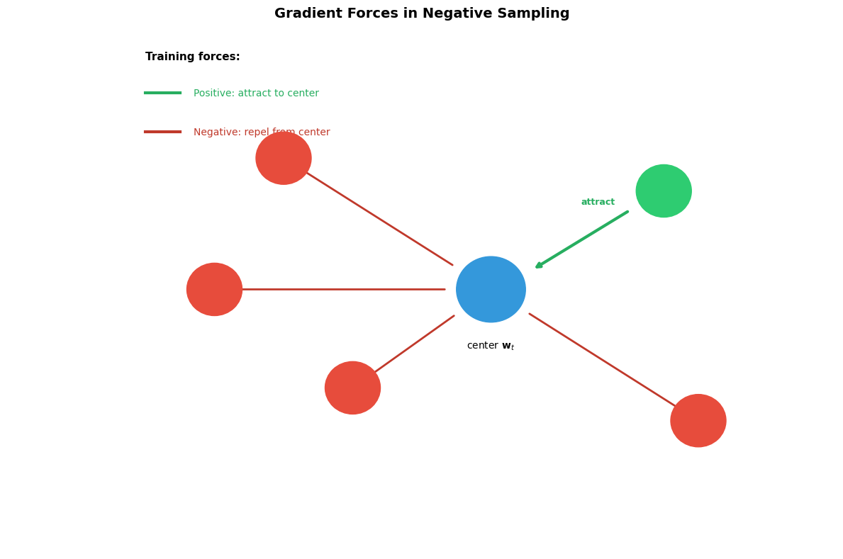
Together, these terms create opposing forces: the first pulls genuine context words toward the center word, while the second pushes random words away. Through millions of such updates, the embedding space self-organizes so that semantically related words cluster together.

With random initial embeddings, the dot products are near zero, producing sigmoid values around 0.5. This means the model is uncertain about all pairs. Training will push these probabilities toward 1 for positive pairs and toward 0 for negatives.

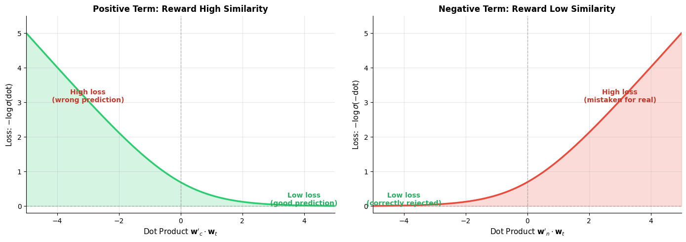
The loss landscape reveals the asymmetric pressure applied by each term. For positive pairs (left), the loss drops sharply as the dot product increases, strongly encouraging the model to push genuine context words closer. For negative pairs (right), the loss drops as the dot product becomes negative, encouraging dissimilar embeddings. The steepest gradients occur near zero, where the model is most uncertain, focusing learning effort where it matters most.

Understanding the Gradient ForcesLink Copied

The objective function creates a tug-of-war in embedding space. Each training step applies forces that reshape the geometry of word representations. Understanding these gradients reveals how semantic structure emerges from local updates.

During backpropagation, two types of forces act on each embedding:

1. Attractive force (positive pairs): The gradient pulls the center word embedding toward its true context word. Words that genuinely co-occur are drawn together in the vector space.

2. Repulsive force (negative pairs): The gradient pushes the center word away from each sampled negative. Words that don't co-occur are separated in the vector space.

The magnitude of each force depends on the current prediction confidence. If the model already confidently predicts a positive pair correctly, the gradient is small. If it's uncertain or wrong, the gradient is large. This self-regulating behavior focuses learning on the most informative examples.

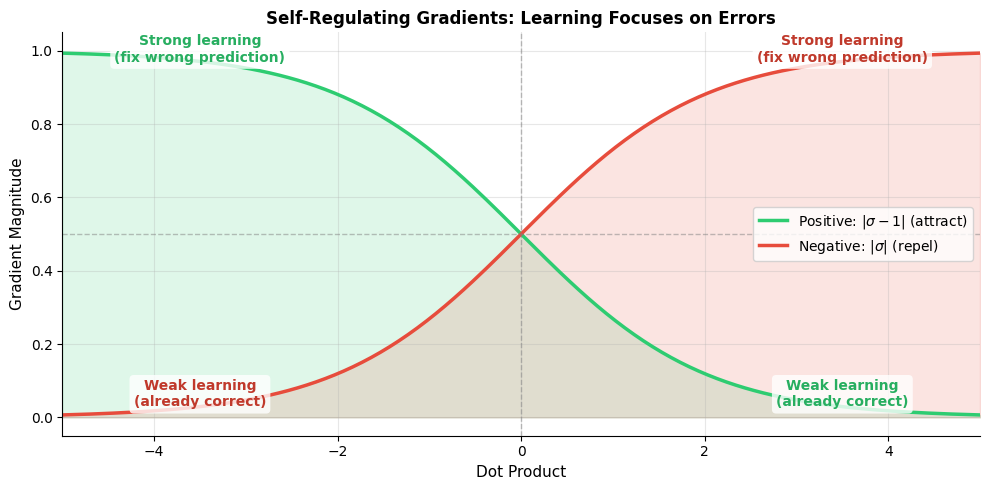
The gradient curves cross at zero, where the model is maximally uncertain. For positive pairs, the model learns strongly when embeddings are dissimilar (negative dot product) but relaxes when they're already similar. For negative pairs, the opposite holds: strong learning when embeddings are incorrectly similar, weak learning when already dissimilar. This elegant self-regulation emerges naturally from the sigmoid function.

Let's derive the gradients explicitly. For the center word embedding $\mathbf{w}_t$:

where:

• $\frac{\partial \mathcal{L}}{\partial \mathbf{w}_t}$: gradient of the objective with respect to the center word embedding
• $\sigma(\mathbf{w}'_c \cdot \mathbf{w}_t)$: sigmoid of the positive pair dot product (current prediction)
• $\sigma(\mathbf{w}'_{n_i} \cdot \mathbf{w}_t)$: sigmoid of the $i$-th negative pair dot product

The first term pulls the center word toward the positive context (since $\sigma - 1 < 0$), while the sum pushes it away from negatives.

For the positive context word embedding $\mathbf{w}'_c$:

This gradient points toward the center word when the prediction is uncertain, pulling the context embedding closer.

For each negative word embedding $\mathbf{w}'_{n_i}$:

This gradient points away from the center word, pushing negative samples to become more dissimilar.

The Sampling Distribution: Why $P_n(w) \propto f(w)^{0.75}$Link Copied

The choice of how to sample negative words turns out to be surprisingly consequential. A naive approach might sample words uniformly at random from the vocabulary. But consider what happens: "the" appears in nearly every sentence, yet it would only be sampled as a negative in $1/V$ of cases. Meanwhile, "aardvark" appears rarely in real text but would be sampled just as often as "the."

This mismatch creates problems. Common function words like "the" genuinely appear near almost every word in the corpus. Sampling them as negatives is confusing because they're often legitimate context words too. Rare words, conversely, might appear as negatives so often that the model learns to push everything away from them, hurting their embedding quality.

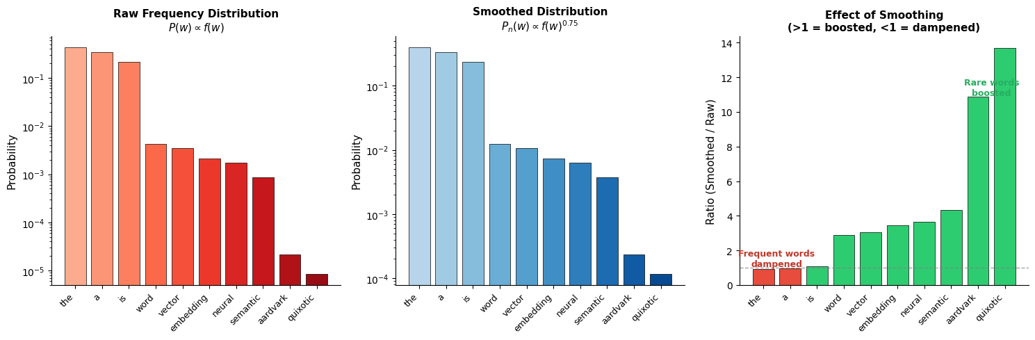
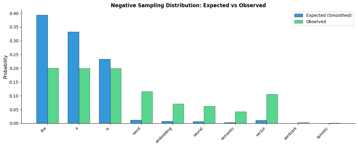
The Word2Vec authors discovered that a modified unigram distribution works best:

where:

• $P_n(w)$: probability of sampling word $w$ as a negative
• $f(w)$: frequency (count) of word $w$ in the corpus
• $0.75$: smoothing exponent (empirically determined)

The exponent 0.75 was determined empirically and has two important effects:

1. Reduces dominance of frequent words: Without the exponent, "the" might account for 7% of the sampling distribution. With 0.75, its share drops, giving other words more representation.

2. Increases representation of rare words: Rare words are sampled more often than pure frequency would suggest, providing better training signal for their embeddings.

The comparison shows how smoothing redistributes probability mass. Common words like "the" drop from dominating the distribution (raw frequency ~43%) to a more moderate share. Rare words like "aardvark" and "quixotic" see their sampling probability increase relative to their raw frequency. This ensures rare words receive adequate negative sampling during training.

Why 0.75? Intuition and AlternativesLink Copied

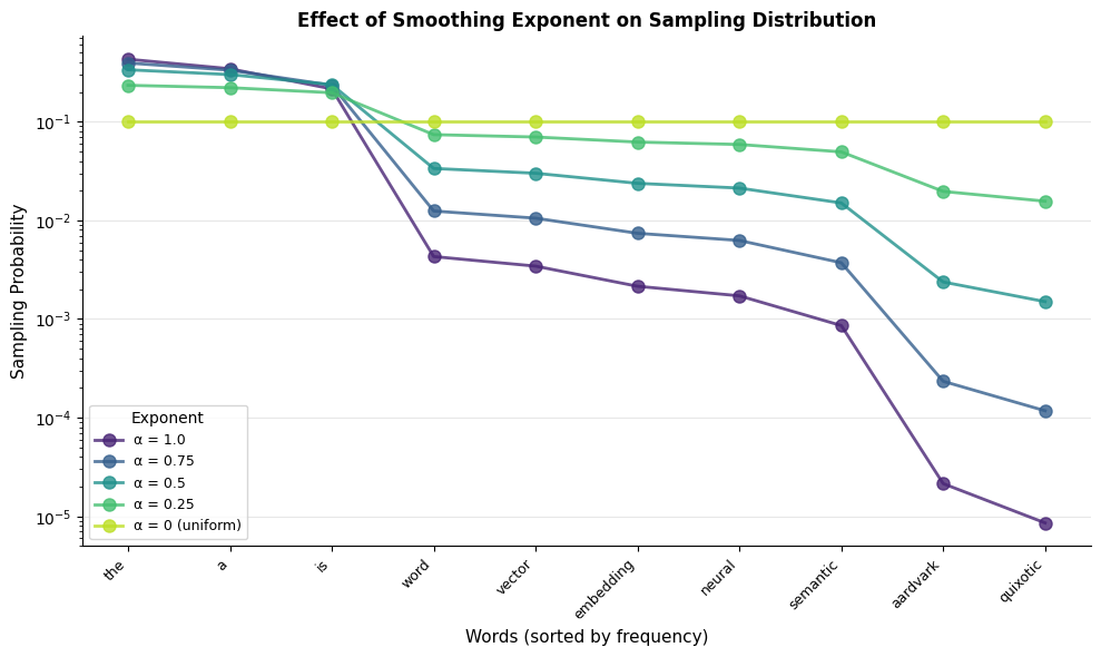
The exponent 0.75 was found empirically by the Word2Vec authors. But why does it work?

• Exponent = 1.0 (raw frequency): Frequent words dominate. The model sees "the" as a negative over and over, wasting computation on words that are already well-positioned.

• Exponent = 0.0 (uniform): Rare words appear as often as frequent ones. But rare words may genuinely share contexts with many other words, making them poor negatives.

• Exponent = 0.75: A compromise. Common words still appear often enough to learn good embeddings, but rare words get meaningful representation in the negative samples.

How Many Negative Samples? The $k$ HyperparameterLink Copied

The number of negative samples $k$ is a crucial hyperparameter. More negatives provide stronger training signal but increase computation time.

The original Word2Vec paper recommends:

• k = 5-10 for large datasets (billions of words)
• k = 15-25 for smaller datasets

The intuition: with more data, each positive example is reinforced many times. Fewer negatives suffice because the model sees the same positive patterns repeatedly. With less data, more negatives help compensate for sparse positive signal.

The speedup is dramatic. For a 100,000-word vocabulary with 10 negative samples, negative sampling performs approximately 9,000 times fewer operations per training step than full softmax. This translates directly to training time: what would take months with softmax can be completed in days with negative sampling.

The trade-off between the number of negative samples and computational cost is linear: doubling $k$ doubles the work per training step. But the relationship between $k$ and embedding quality is more nuanced, with diminishing returns as $k$ increases.

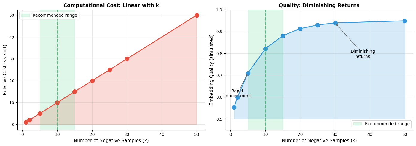
The recommended range of k=5-15 captures most of the quality gains while keeping computational costs manageable. Beyond k=20, additional negatives provide minimal improvement but continue to increase training time linearly.

Noise Contrastive Estimation: The Theoretical FoundationLink Copied

Negative sampling didn't emerge from thin air. It's a practical simplification of a more principled technique called Noise Contrastive Estimation (NCE), developed by Gutmann and Hyvärinen (2010). Understanding NCE illuminates why negative sampling works and what theoretical guarantees we sacrifice for efficiency.

The core insight of NCE is simple: if you can perfectly distinguish real data from noise, you must have learned what makes the data real. Here's how it works:

1. Draw positive samples from the true data distribution $P_d(w | c)$ (context words given center)
2. Draw negative samples from a known noise distribution $P_n(w)$
3. Train a classifier to distinguish them

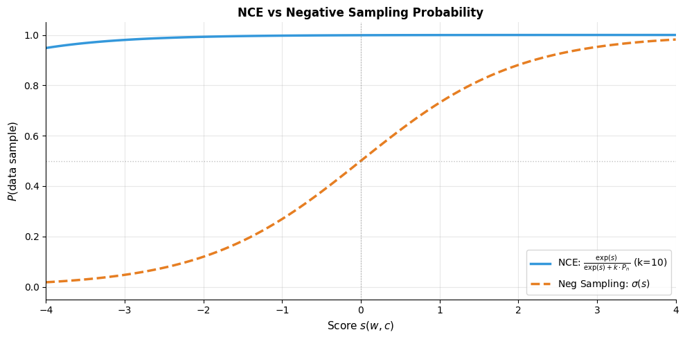
The key insight: if we use $k$ noise samples for every data sample, and our model outputs $s(w, c)$ as a score, the optimal classification decision is:

where:

• $P_d(w | c)$: true data distribution (probability of word $w$ given context $c$)
• $P_n(w)$: noise distribution probability for word $w$

NCE models this probability as:

where:

• $s(w, c)$: the model's score for word pair $(w, c)$, typically the dot product $\mathbf{w}' \cdot \mathbf{c}$
• $k$: number of noise samples per data sample
• $P_n(w)$: probability of word $w$ under the noise distribution

When training converges, the model learns that $\exp(s(w, c)) \propto P_d(w | c)$, recovering the true distribution up to a constant.

From NCE to Negative SamplingLink Copied

Negative sampling departs from NCE in two important ways, each trading theoretical rigor for practical efficiency:

First simplification: Ignoring the partition function. NCE explicitly models the normalization constant (the sum over all vocabulary words that makes probabilities sum to 1). This constant is precisely what makes softmax expensive. Negative sampling simply ignores it, treating $\exp(s(w, c))$ as an unnormalized score. We lose the ability to compute true probabilities, but for learning embeddings, relative scores suffice.

Second simplification: Using sigmoid directly. NCE's probability formula accounts for the ratio of data to noise samples and the noise distribution. Negative sampling replaces this with the simpler sigmoid $\sigma(s(w, c))$. This makes implementation straightforward and gradients clean, at the cost of some theoretical precision.

What do we lose? Negative sampling no longer guarantees convergence to the true data distribution. The embeddings might not represent exact co-occurrence probabilities. But for downstream tasks like analogy completion, similarity search, and transfer learning, this rarely matters. The embeddings capture semantic relationships just as well, at a fraction of the computational cost.

Implementing Efficient Negative SamplingLink Copied

A practical implementation needs efficient sampling from the noise distribution. Computing probabilities for 100,000 words every time we need a sample is slow. Instead, we precompute a sampling table.

The Alias MethodLink Copied

The most efficient approach uses the alias method, which allows $O(1)$ sampling from any discrete distribution after $O(V)$ preprocessing. However, a simpler approach that's nearly as fast uses cumulative probabilities:

Verifying the Sampling DistributionLink Copied

Let's verify that our sampler matches the intended distribution:

Complete Negative Sampling ImplementationLink Copied

Now let's put everything together into a complete, trainable Skip-gram model with negative sampling:

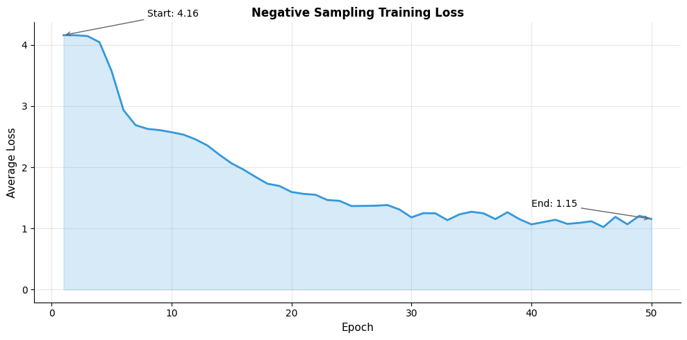
Training with Negative SamplingLink Copied

Let's train our model on a corpus with clear semantic structure:

The loss decreases substantially over training, indicating the model is learning to distinguish positive from negative pairs. The reduction from initial to final loss shows the embeddings have organized to reflect the corpus structure.

Evaluating the Learned EmbeddingsLink Copied

Let's examine whether the model has learned meaningful semantic relationships:

Visualizing the Embedding SpaceLink Copied

Similarity HeatmapLink Copied

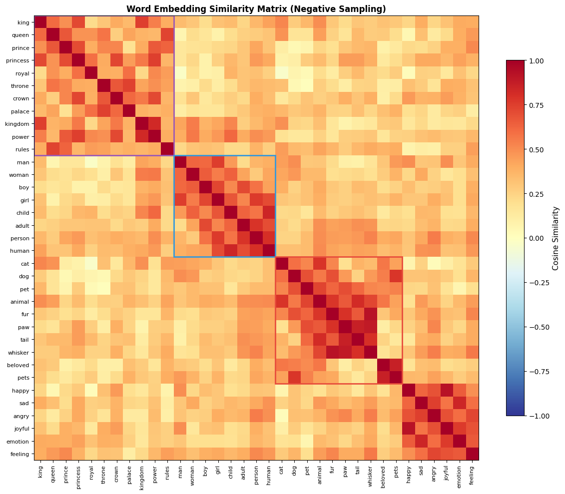
Comparing Full Softmax and Negative SamplingLink Copied

How do embeddings from negative sampling compare to those from full softmax? Let's train both on the same data:

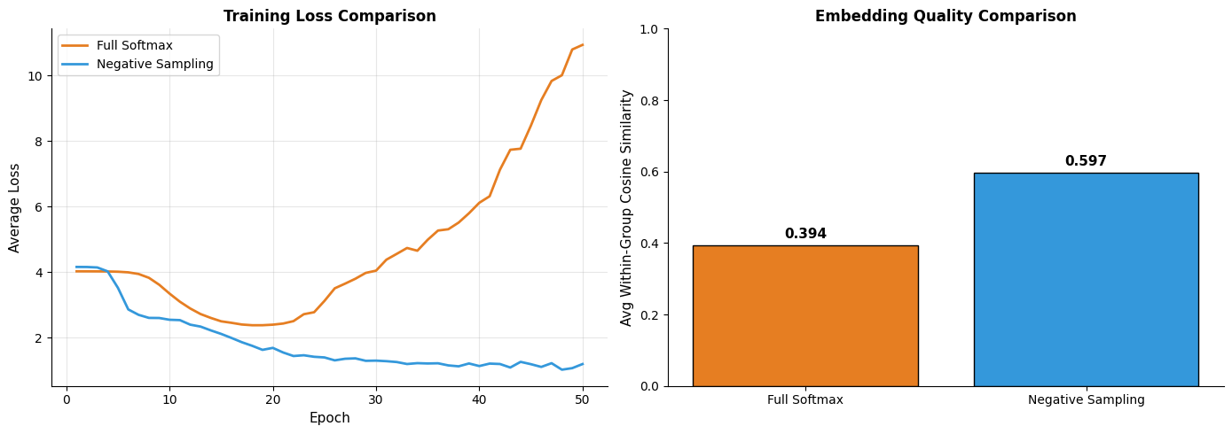
The comparison reveals a key insight: negative sampling produces embeddings of similar quality to full softmax, despite using a fundamentally different (and much cheaper) objective. This explains why negative sampling became the default training method for Word2Vec and similar models.

Training Dynamics VisualizationLink Copied

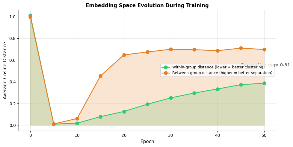
Training progressively separates semantic clusters. Initially, within-group and between-group distances are similar because embeddings are random. As training proceeds, related words (within same semantic group) move closer together while unrelated words (across groups) move apart. The growing gap between these curves indicates successful learning.

Practical ConsiderationsLink Copied

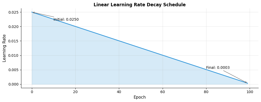
Learning Rate SchedulingLink Copied

The original Word2Vec implementation uses linear learning rate decay:

Subsampling Frequent WordsLink Copied

Very frequent words like "the" and "a" provide less information than rare words. Word2Vec subsamples frequent words during training.

where:

• $P(\text{keep } w)$: probability of keeping word $w$ during training
• $f(w)$: relative frequency of word $w$ in the corpus (count of $w$ divided by total word count)
• $t$: subsampling threshold, typically $10^{-5}$

Words with frequency above the threshold $t$ get subsampled, while rare words are always kept. This formula ensures that very frequent words like "the" appear less often during training, reducing their dominance while preserving rare word information.

The most frequent words like "the" and "a" have very low keep probabilities, meaning they're discarded during most training iterations. This prevents them from overwhelming the training signal. Rarer words like "aardvark" and "quixotic" have keep probability 1.0, ensuring every occurrence contributes to their embeddings.

Mini-batch TrainingLink Copied

For large-scale training, processing one pair at a time is inefficient. Mini-batch training processes multiple pairs simultaneously, enabling better hardware utilization:

Limitations and ExtensionsLink Copied

Negative sampling made Word2Vec practical, but it has limitations:

Approximation quality: Negative sampling doesn't optimize the true softmax objective. For most applications, this doesn't matter, but tasks requiring precise probability estimates may suffer.

Hyperparameter sensitivity: The choice of $k$ (number of negatives) and $\alpha$ (smoothing exponent) affect results. The defaults (k=5-10, $\alpha$=0.75) work well but aren't universally optimal.

No guarantee of convergence to NCE solution: Unlike NCE, negative sampling doesn't have theoretical guarantees about recovering the true distribution. In practice, this rarely matters for downstream tasks.

Static embeddings: Like all Word2Vec variants, negative sampling produces static embeddings. Each word gets one vector regardless of context. Modern contextual models like BERT address this limitation.

SummaryLink Copied

Negative sampling transforms the Skip-gram training problem from an expensive multi-class classification (softmax over vocabulary) to efficient binary classification (real vs. fake pairs). This simple change reduces computational complexity from $O(V)$ to $O(k)$ per training step, making large-scale training feasible.

Key takeaways:

• Binary classification reformulation: Instead of predicting which word is the context, predict whether a given pair is genuine or randomly sampled
• Sigmoid instead of softmax: Each pair is scored independently using the sigmoid function, eliminating the need to normalize over the entire vocabulary
• The sampling distribution matters: Using $P_n(w) \propto f(w)^{0.75}$ balances representation between frequent and rare words
• Number of negatives ($k$): Typically 5-20, with smaller values for larger datasets. More negatives provide stronger training signal at higher computational cost
• Theoretical foundation in NCE: Negative sampling is a simplification of Noise Contrastive Estimation, trading theoretical guarantees for practical efficiency
• Comparable quality to full softmax: Despite the approximation, embeddings from negative sampling rival those from full softmax in downstream tasks

The next chapter explores hierarchical softmax, an alternative approximation that organizes the vocabulary as a binary tree, reducing softmax complexity from $O(V)$ to $O(\log V)$.

Key ParametersLink Copied

Negative Sampling Parameters:

• num_negatives (k): Number of negative samples per positive pair. Use 5-10 for large corpora (billions of words), 15-25 for smaller datasets. More negatives provide stronger training signal but increase computation.

• alpha (smoothing exponent): Controls the noise distribution shape. The standard value 0.75 balances sampling frequency between common and rare words. Lower values (0.5) boost rare words more; higher values (1.0) sample proportionally to frequency.

• embedding_dim: Dimensionality of word vectors. Typical values range from 50-300. Larger dimensions capture more nuance but require more data and computation.

• learning_rate: Step size for gradient updates. Start with 0.025 and decay linearly to 0.0001. Higher rates speed early training; lower rates enable fine-tuning.

• window_size: Context window for extracting training pairs. Common values are 5-10. Larger windows capture broader semantic relationships; smaller windows focus on syntactic patterns.

• subsampling_threshold (t): Threshold for discarding frequent words. Typical value is $10^{-5}$. Words more frequent than this are probabilistically skipped during training.

• epochs: Number of passes through the training data. For large corpora, 1-5 epochs often suffice. Smaller datasets may benefit from 20-50 epochs.

QuizLink Copied

Ready to test your understanding? Take this quick quiz to reinforce what you've learned about negative sampling.