

A comprehensive guide to the Skip-gram model from Word2Vec, covering architecture, objective function, training data generation, and implementation from scratch.

This article is part of the free-to-read Language AI Handbook
Choose your expertise level to adjust how many terms are explained. Beginners see more tooltips, experts see fewer to maintain reading flow. Hover over underlined terms for instant definitions.
Skip-gram Model
The distributional hypothesis tells us that words appearing in similar contexts have similar meanings. But how do we turn this insight into practical word representations? Co-occurrence matrices capture contextual patterns, but they're sparse, high-dimensional, and computationally expensive. What if we could learn dense, low-dimensional vectors that encode the same distributional information more efficiently?
In 2013, Mikolov et al. introduced Word2Vec, a family of neural network models that changed how we create word representations. The Skip-gram model, one of the two Word2Vec architectures, takes a simple approach: given a word, predict its context. By training a neural network on this task across billions of words, we learn dense vectors that capture rich semantic relationships. Words like "king" and "queen" end up close together in vector space. Vector arithmetic even works: .
This chapter introduces the Skip-gram architecture from the ground up. We'll build intuition for why predicting context words leads to meaningful representations, work through the mathematics step by step, and implement a working Skip-gram model from scratch.
The Core Idea: Predicting Context from Words
Traditional distributional methods count co-occurrences and store them in massive matrices. Skip-gram flips the script: instead of counting, we predict. Given a target word, the model tries to predict which words appear nearby in the training corpus.
The Skip-gram model learns word representations by training a neural network to predict context words given a center word. The learned weights of this network become the word embeddings.
Consider the sentence: "The quick brown fox jumps over the lazy dog." If we take "fox" as our target word with a context window of size 2, Skip-gram asks: given "fox," can we predict that "brown," "quick," "jumps," and "over" appear nearby?
The model learns by trying to maximize the probability of these context words given the target. If "fox" frequently appears near "brown" in the training corpus, the model adjusts its weights to make high. Through millions of such updates, words that appear in similar contexts develop similar vector representations.
Architecture: Two Embedding Matrices
The Skip-gram architecture is simple: a shallow neural network with a single hidden layer and no activation function. The key insight lies in what we do with the learned weights.
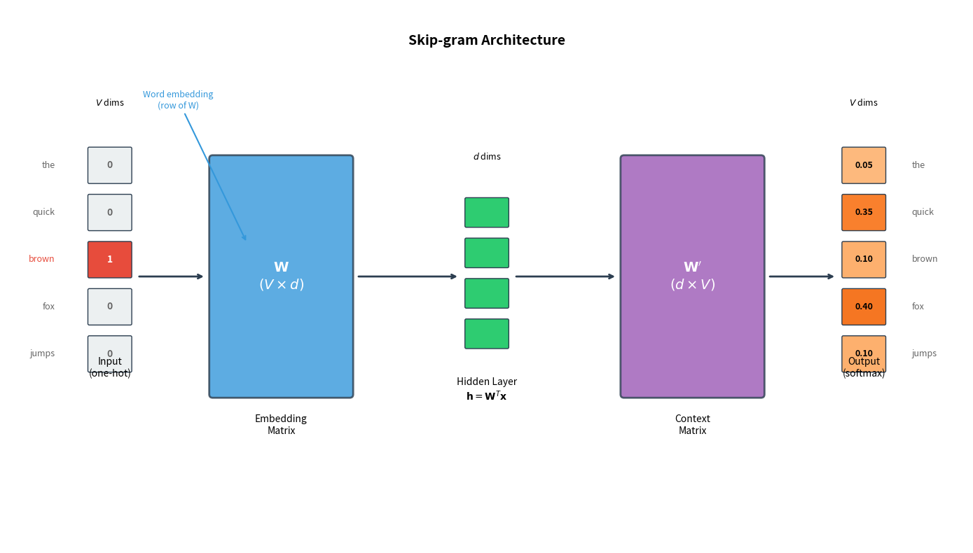
The network has two weight matrices:
-
Embedding matrix (size ): Maps input words to dense vectors. Each row is the embedding for one vocabulary word. When we input a one-hot vector for word , multiplying by simply selects the corresponding row.
-
Context matrix (size ): Maps the hidden representation to output scores. Each column represents a word as a potential context.
Here is the vocabulary size (often 100,000+ words) and is the embedding dimension (typically 100-300).
With 2 million parameters, Skip-gram is lightweight compared to modern language models. This efficiency comes from the shallow architecture: just two matrix multiplications with no hidden layers or activation functions. Despite this simplicity, Skip-gram learns rich representations.
Skip-gram maintains separate embeddings for words as targets () and as contexts (). After training, we typically use only the embedding matrix as our word vectors, though some implementations average both matrices or concatenate them.
Input and Output Representations
Understanding how Skip-gram represents words at input and output is essential for grasping the model's mechanics. The input uses sparse one-hot vectors that serve as lookup indices, while the output produces probability distributions over the entire vocabulary.
One-Hot Encoding
The input to Skip-gram is a one-hot encoded vector. For a vocabulary of words, each word is represented as a vector of length with a single 1 at the word's index and 0s everywhere else.
The one-hot vector is extremely sparse: 7 zeros and a single 1. For a real vocabulary of 100,000 words, each input would have 99,999 zeros. This sparsity is why the embedding lookup is so efficient: multiplying by a one-hot vector simply selects one row.
From One-Hot to Embedding
When we multiply the one-hot vector by the embedding matrix , something useful happens: we simply extract the row corresponding to our input word. The hidden layer representation is computed as:
where:
- : the hidden layer vector (the word embedding), with dimension
- : the embedding matrix of size , where each row is a word's embedding
- : a one-hot encoded input vector of length with a single 1 at the word's position
- : the vocabulary size
- : the embedding dimension
If is one-hot with a 1 at position , then is exactly the -th row of . This is why we call the "embedding matrix": its rows are the word embeddings.
The direct row selection W[idx] is computationally equivalent to the matrix multiplication W.T @ one_hot but far more efficient. In practice, embedding layers in deep learning frameworks use this lookup optimization rather than actual matrix multiplication.
Output Scores and Softmax
The hidden vector is then projected through the context matrix to produce a score for each vocabulary word. These raw scores (called "logits") indicate how compatible each word is as a context:
where:
- : the output score vector of length , with one score per vocabulary word
- : the context matrix of size , where each column is a word's context representation
- : the hidden layer (the center word's embedding)
Each element represents how likely word is to be a context word. Higher scores indicate stronger compatibility. To convert these scores to a valid probability distribution, we apply the softmax function:
where:
- : the probability of observing word as a context word given center word
- : the input (center) word
- : a candidate context word
- : the embedding vector of the input word (row of )
- : the context vector of word (column of )
- : the raw score for word , computed as the dot product of the context and embedding vectors
- : the vocabulary size
- : the exponential function, which ensures all values are positive
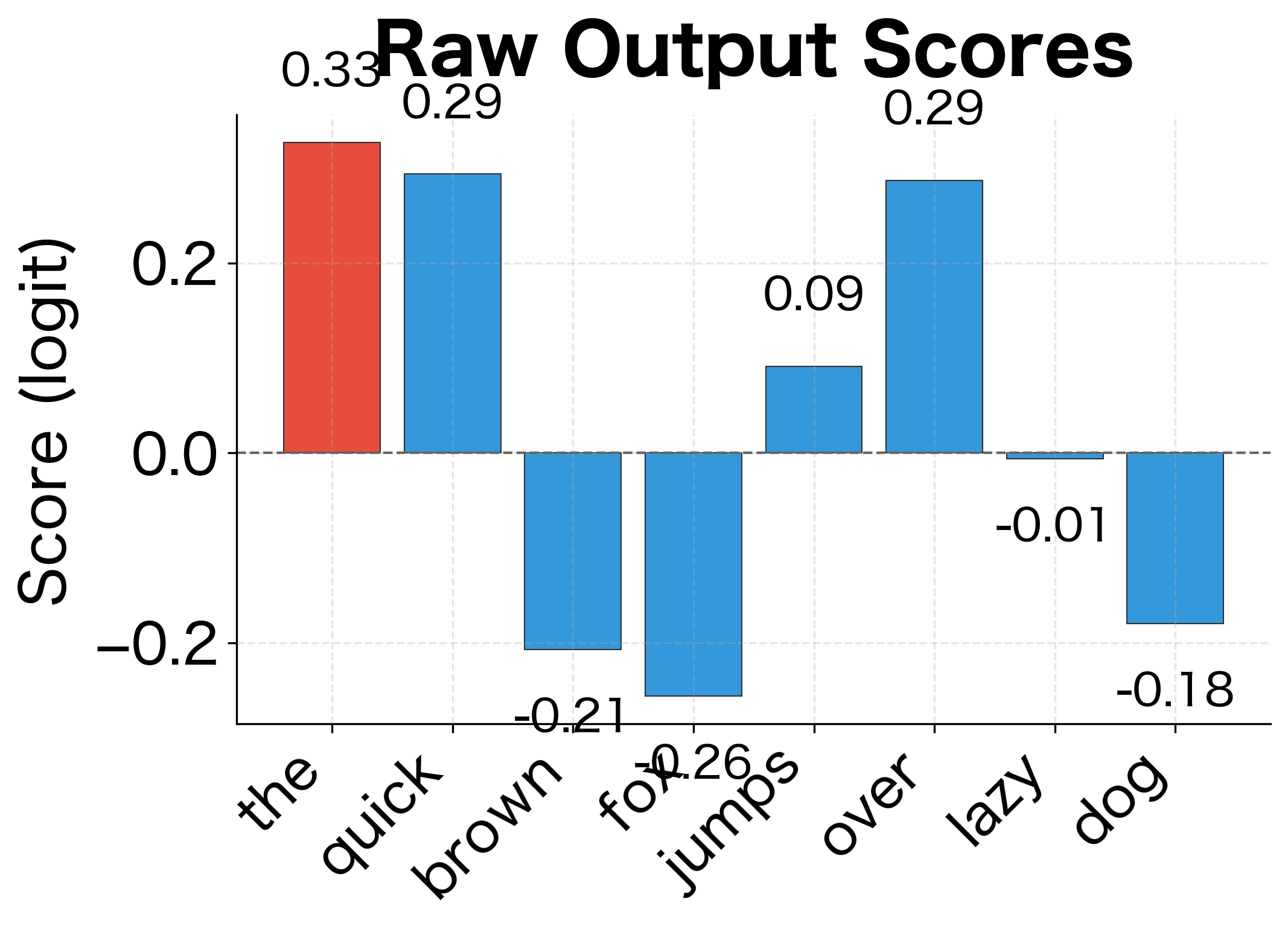
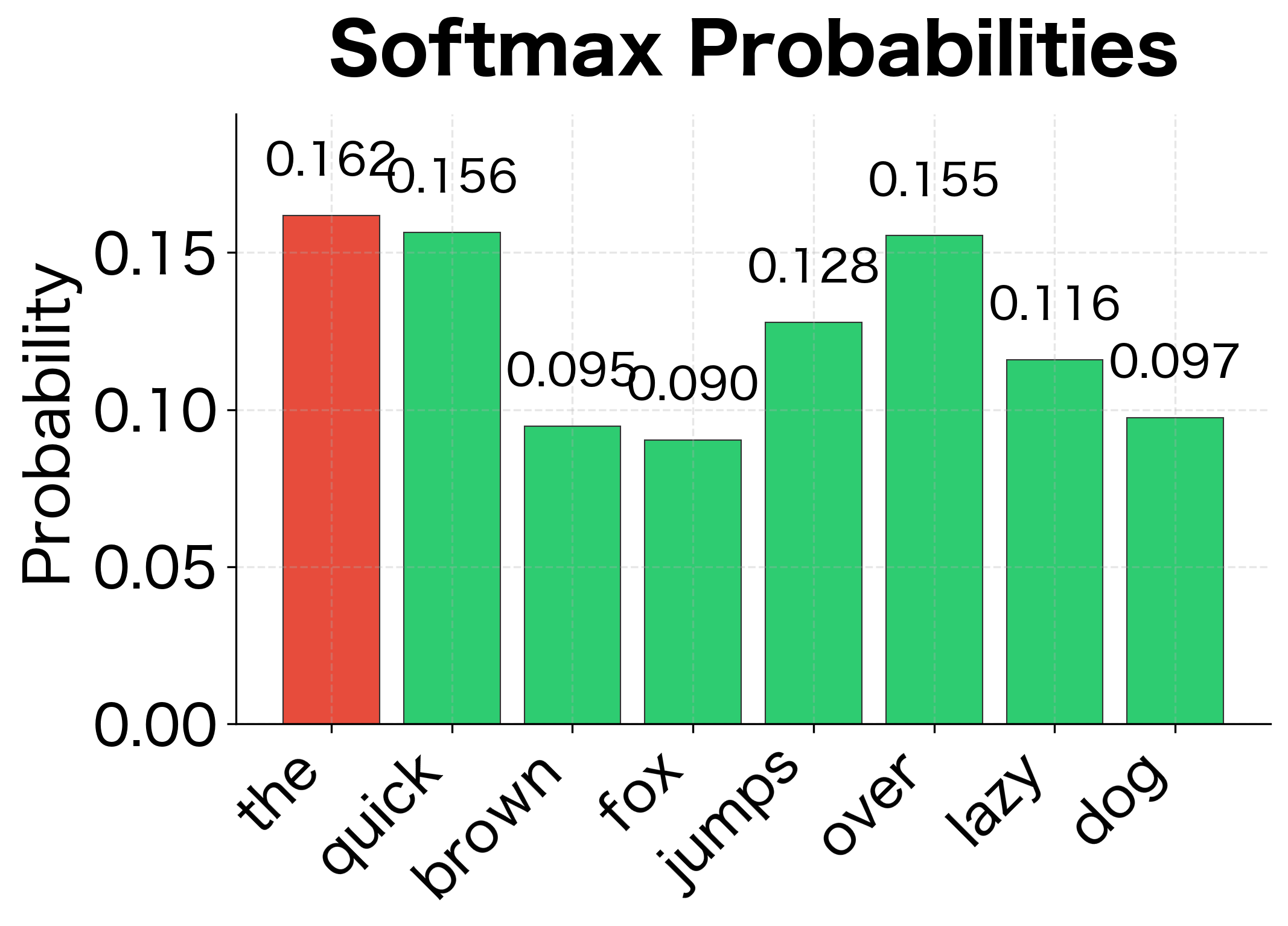
The softmax function has two key properties: (1) it transforms any real-valued scores into positive numbers that sum to 1, creating a valid probability distribution, and (2) it amplifies differences between scores, with larger scores receiving disproportionately more probability mass due to the exponential function.
The raw scores (logits) can be any real number, positive or negative. Softmax transforms them into a valid probability distribution: all values between 0 and 1, summing to exactly 1. Notice how the word with the highest score gets a disproportionately large probability. This "winner-take-more" behavior is characteristic of the exponential function in softmax.
Understanding softmax behavior matters because it determines how the model distributes probability mass. The exponential function amplifies differences: even small gaps in raw scores become large probability differences. This property helps the model make confident predictions but also creates computational challenges we'll address later.
The Skip-gram Objective Function
We've seen how Skip-gram transforms words into vectors and predicts context probabilities. But how does the model actually learn? What signal tells it whether its current embeddings are good or bad? The answer lies in the objective function: a mathematical expression that quantifies how well the model's predictions match reality.
From Intuition to Formalization
Let's build the objective function step by step, starting from a simple intuition.
The core insight: If our embeddings are good, then given a center word, the model should assign high probability to words that actually appear nearby and low probability to words that don't. The objective function formalizes this: we want to maximize the probability of observing the actual context words.
Consider our running example: the sentence "The quick brown fox jumps over the lazy dog." When "fox" is the center word with a window of size 2, the true context words are "quick," "brown," "jumps," and "over." A well-trained model should predict:
- → high
- → high
- → low
The Probability of Context Words
For a single center word at position , we observe context words at positions (where is the window size). Skip-gram assumes these context words are conditionally independent given the center word, so the probability of observing all of them is the product of individual probabilities:
where:
- : the product operator, multiplying together all the terms
- : the window size (number of context words on each side of the center word)
- : the offset from the center position, ranging from to but excluding 0 (the center word itself)
- : the center word at position
- : the context word at position (i.e., positions away from the center)
- : the probability of observing context word given center word
For a window size of , this product includes probabilities for positions , giving us four context words per center word.
The product form comes from the independence assumption: we treat each context position as a separate prediction task. While context words aren't truly independent (knowing "brown" appears near "fox" tells us something about what other words might appear), this simplification makes training tractable and works well in practice.
Converting to Log-Likelihood
Working with products of probabilities is numerically unstable. Multiplying many small numbers quickly underflows to zero. The standard solution is to take the logarithm, which converts products to sums. Using the property , we transform the product of probabilities into a sum of log-probabilities:
where:
- : the log-likelihood for center word at position (a scalar value)
- : the summation operator, adding together all the terms
- : the window size
- : the offset from the center position, excluding 0
- : the log-probability of observing context word given center word
This is the log-likelihood for a single center word. Since probabilities are between 0 and 1, their logarithms are negative, but higher (less negative) values mean the model assigns higher probabilities to the true context words. Our goal is to maximize this quantity.
Unpacking the Softmax
Recall that is computed via softmax over dot products:
where:
- : the embedding vector of the center word (from matrix )
- : the context vector of the context word at position (from matrix )
- : the dot product between context and embedding vectors (a scalar score)
- : the exponential function
- : the vocabulary size
- : an index iterating over all vocabulary words in the normalization sum
Substituting this into our log-likelihood and using the property , we get:
where:
- : the score for the true context word (the "positive" term we want to maximize)
- : the log-sum-exp over all vocabulary words (the normalization term)
This expanded form reveals the two forces at work during training:
-
The positive term : Maximizing this pushes the context word's vector closer to the center word's embedding . The dot product increases when vectors point in similar directions.
-
The normalization term : This term is subtracted, so maximizing the objective means minimizing this sum. Since the sum includes all vocabulary words, this effectively pushes all other words away from the center word.
The interplay between these forces is what makes Skip-gram work: it simultaneously pulls true context words closer while pushing non-context words away.
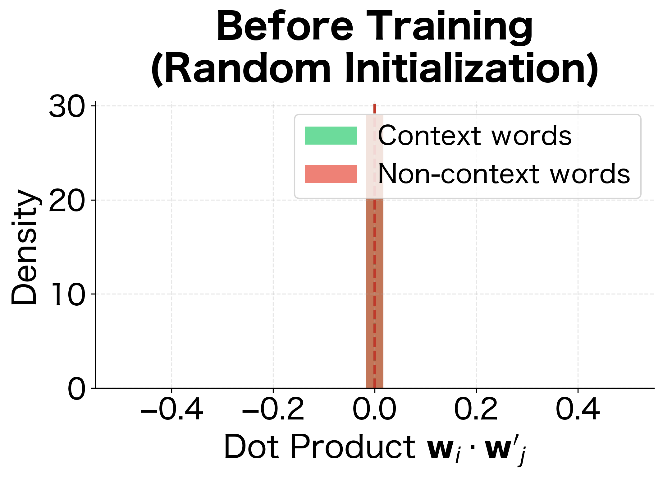
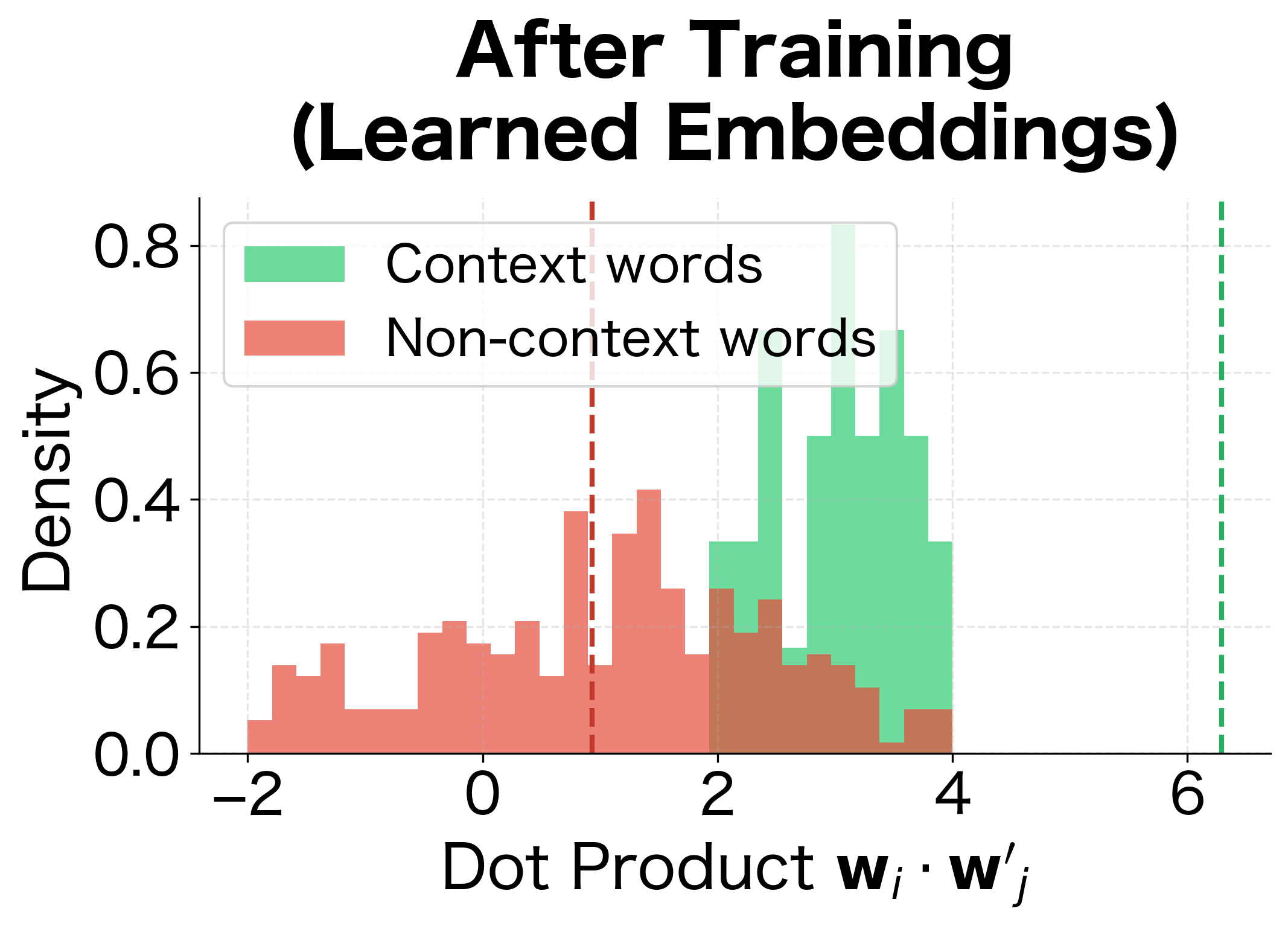
This visualization shows exactly what Skip-gram learns to do: before training, dot products between any word pair are randomly distributed around zero. After training, the distributions separate. Context words (which should have high probability) develop higher dot products, while non-context words have lower dot products. This separation is what enables the softmax to assign high probabilities to true context words.
The Full Corpus Objective
A single center word gives us one training signal. To learn robust embeddings, we aggregate over the entire corpus. If the corpus has words total, we average the log-likelihood across all positions:
where:
- : the objective function (average log-likelihood across the corpus)
- : total number of words in the training corpus
- : position of the current center word (ranging from 1 to )
- : window size (number of context words on each side)
- : offset from the center position, excluding 0
- : the word at position (center word)
- : a context word at offset from position
- : the model's predicted probability for the context word given the center word
The factor normalizes by corpus size, making the objective comparable across different training sets. This is what we maximize during training. In practice, we minimize the negative log-likelihood (cross-entropy loss), which is equivalent but aligns with the convention of "minimizing loss."
Implementing the Loss Function
Let's translate this mathematics into code. The loss function computes how poorly the model predicts context words for a given center word:
The computed loss tells us how surprised the model is by the actual context words. The random baseline represents the expected loss if all words were equally likely, calculated as . Since our loss is close to this baseline with randomly initialized weights, the model is essentially guessing. Lower loss indicates better context predictions.
As training progresses, the model learns to assign higher probabilities to actual context words, driving the loss down. A well-trained model on a large corpus typically achieves losses in the range of 2-4 (when using negative sampling), indicating it has learned to predict context words much better than chance.
Visualizing Gradient Updates
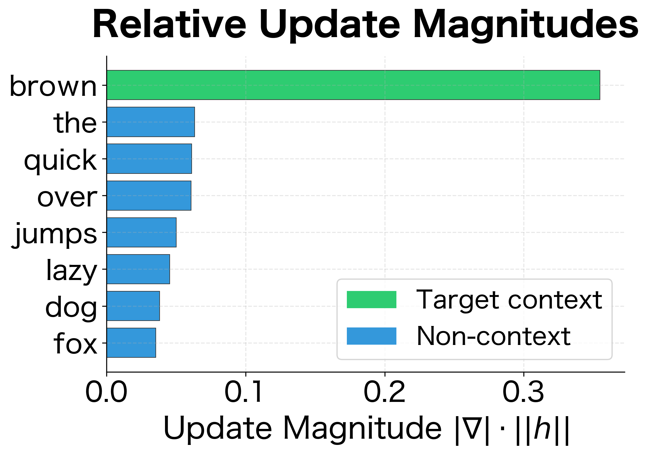
To understand how Skip-gram learns, let's visualize what happens during a single gradient update. When we train on the pair ("fox" → "brown"), the gradients adjust the embeddings:
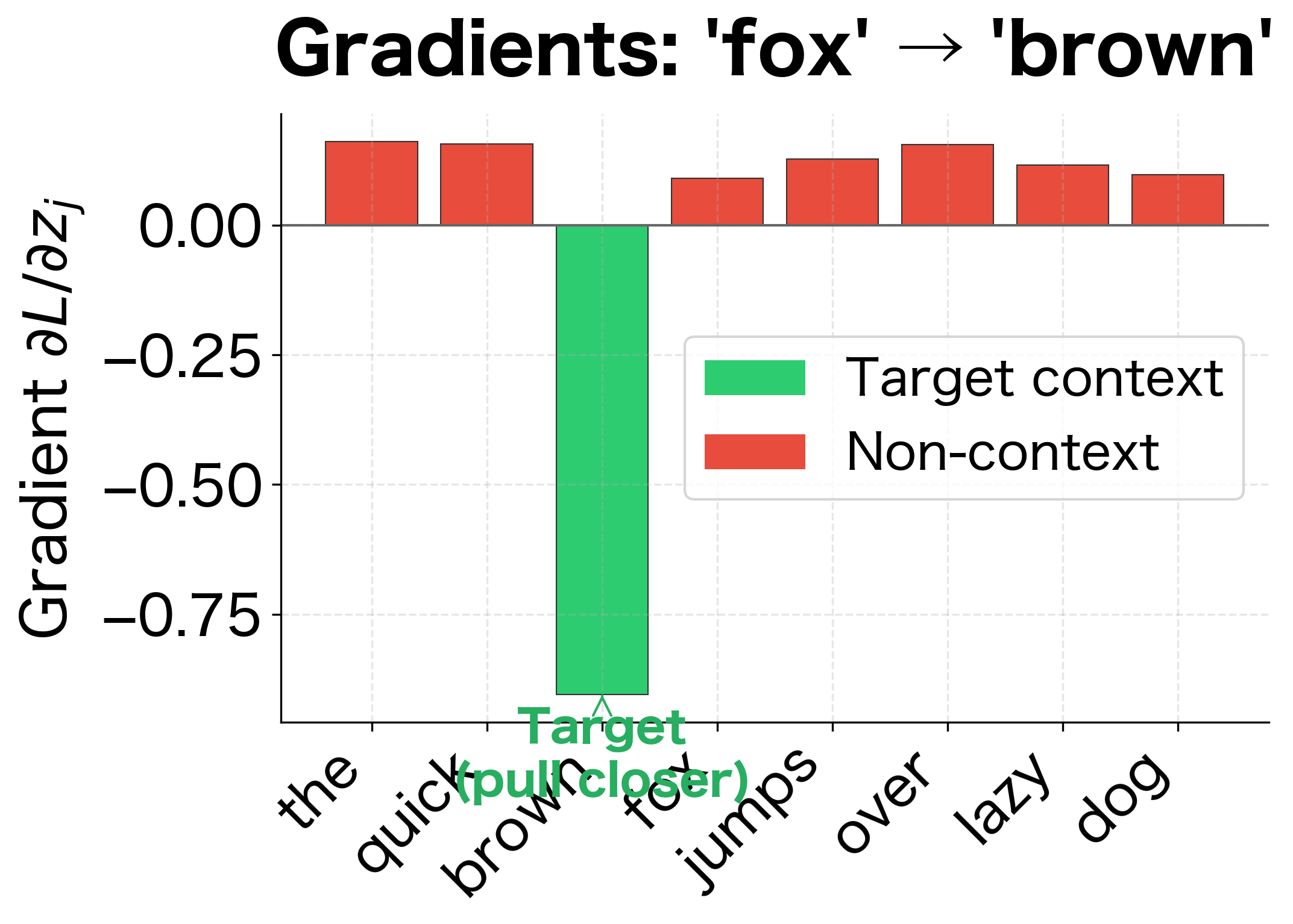
The gradient visualization reveals the core learning mechanism:
- The target context word ("brown") receives a negative gradient, meaning its context vector will be updated to increase its dot product with "fox", pulling it closer in embedding space.
- All other words receive positive gradients proportional to their current probability. Words the model incorrectly thinks are likely contexts get pushed away more strongly.
This push-pull dynamic, repeated millions of times across the corpus, gradually organizes the embedding space so that words appearing in similar contexts end up nearby.
Generating Training Data
With the objective function defined, we need training data to optimize it. Skip-gram's training data consists of (center word, context word) pairs extracted from raw text. The advantage of this approach is that we need no manual labels. The text itself provides supervision through co-occurrence patterns.
The Sliding Window Approach
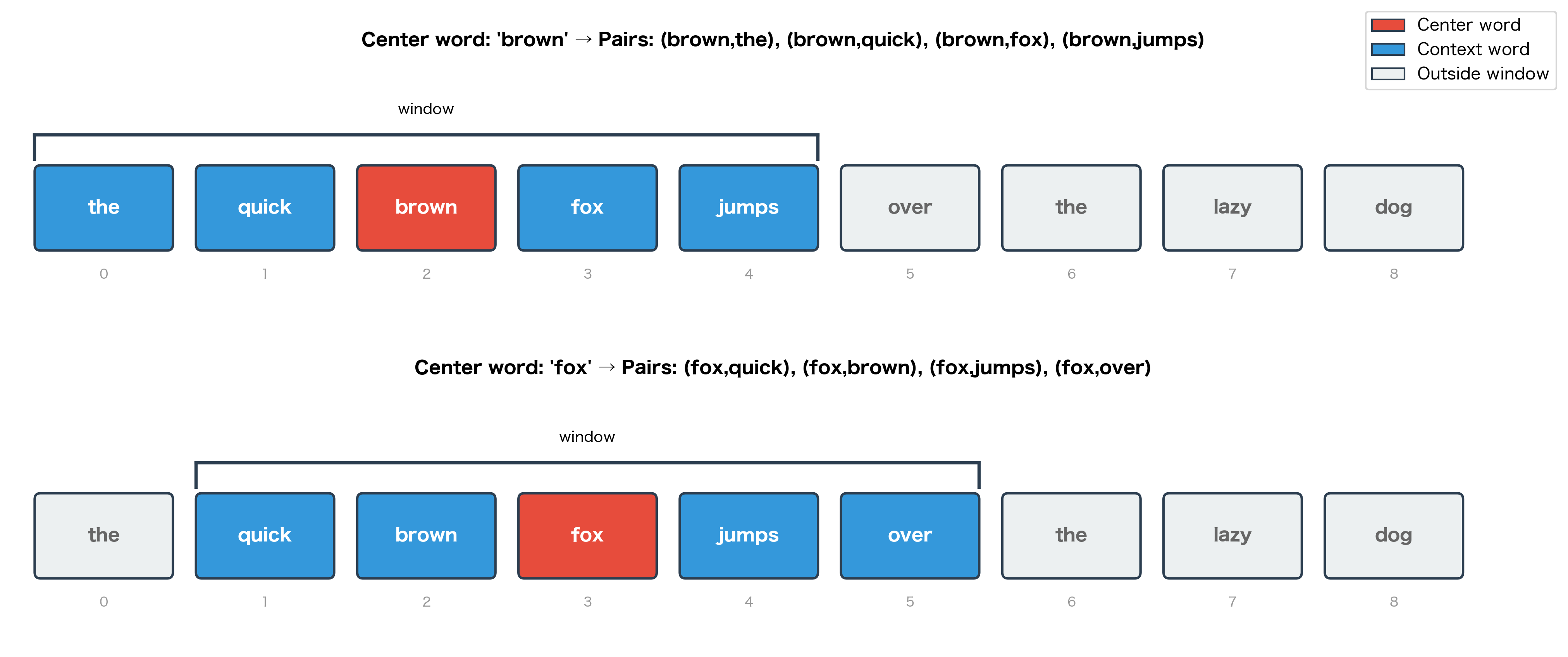
The algorithm is straightforward:
- Slide a window across the corpus, one word at a time
- Treat each word as a potential center word
- Pair it with every word within the window (excluding itself)
This process transforms unstructured text into structured training examples.
The Multiplication Effect
Notice the dramatic expansion: a 9-word sentence produces 30 training pairs. This happens because:
- Each word in the middle of the sentence generates 4 pairs (2 words on each side)
- Words at the edges generate fewer pairs (only 2-3, depending on position)
For large corpora with billions of words, this multiplication effect produces massive training datasets. A corpus of 1 billion words with window size 5 generates roughly 10 billion training pairs. This abundance of training signal is why Skip-gram can learn rich semantic representations without any manual annotation. The structure of language itself provides the supervision.
Window Size: A Critical Hyperparameter
The window size determines how many words on each side of the center word count as context. This choice significantly affects what the embeddings capture.
The window size hyperparameter controls the trade-off between syntactic and semantic similarity in learned embeddings. Smaller windows emphasize syntactic relationships, while larger windows capture topical similarity.
Larger windows create more training pairs, but they may dilute the signal by including less relevant contexts. The trade-off becomes clear: a window of 5 generates roughly 3x more pairs than a window of 1, but those additional context words are further from the center and may be less semantically related.
Small windows (1-2 words) tend to produce embeddings where syntactically similar words cluster together. Words that can substitute for each other in the same grammatical position (like "dog" and "cat" as nouns) end up nearby.
Large windows (5-10 words) capture topical similarity. Words that appear in the same documents or discuss the same subjects cluster together, even if they play different grammatical roles.
Skip-gram vs CBOW: Two Sides of the Same Coin
Word2Vec actually includes two architectures: Skip-gram and Continuous Bag of Words (CBOW). They're mirror images of each other:
- Skip-gram: Given center word, predict context words
- CBOW: Given context words, predict center word
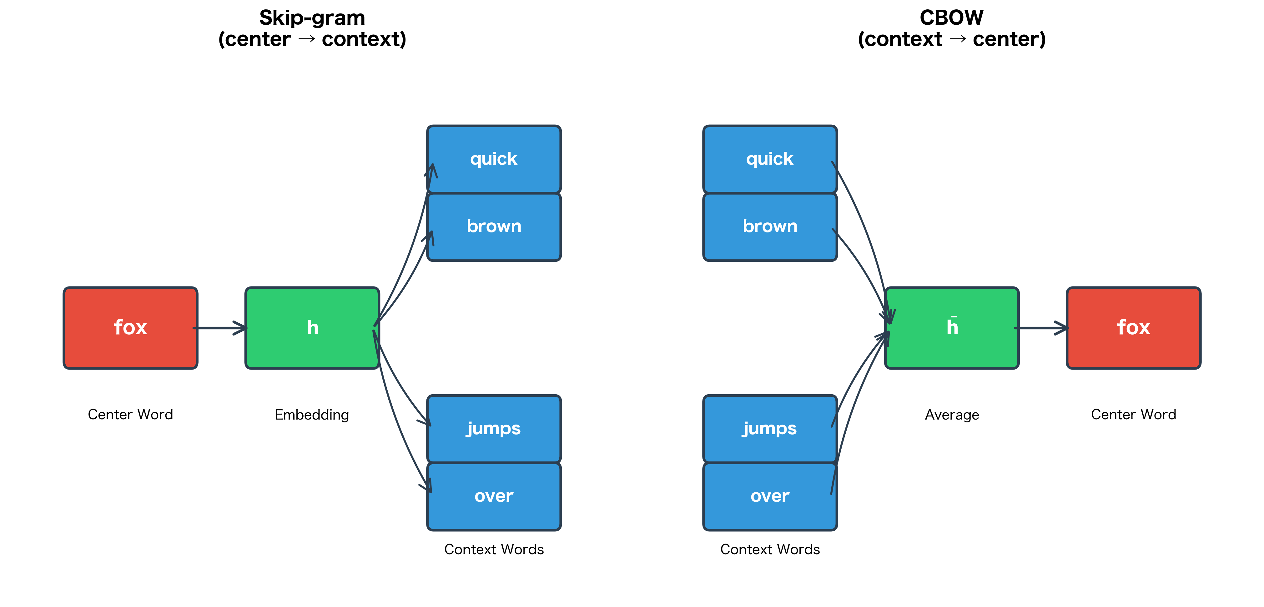
The key differences:
| Aspect | Skip-gram | CBOW |
|---|---|---|
| Input | Single center word | Multiple context words |
| Output | Multiple context words | Single center word |
| Rare words | Better (each occurrence creates multiple training examples) | Worse (rare words get averaged out) |
| Training speed | Slower (more predictions per position) | Faster (one prediction per position) |
| Best for | Smaller datasets, rare words | Larger datasets, frequent words |
Skip-gram's advantage with rare words comes from its training structure. For each occurrence of a rare word, Skip-gram generates multiple training examples (one for each context word). CBOW, by contrast, uses each occurrence only once. This gives Skip-gram more signal for learning good representations of infrequent words.
A Complete Implementation
We've covered the theory: the architecture, the objective function, and the training data. Now let's bring it all together into a working implementation that you can run and experiment with.
The SkipGram Class
Our implementation encapsulates the complete Skip-gram model in a single class. Each method corresponds to a concept we've discussed:
Training the Model
Now let's train our Skip-gram model on a small corpus designed to have clear semantic groupings. We'll use words from five categories: royalty, people, animals, emotions, and movement.
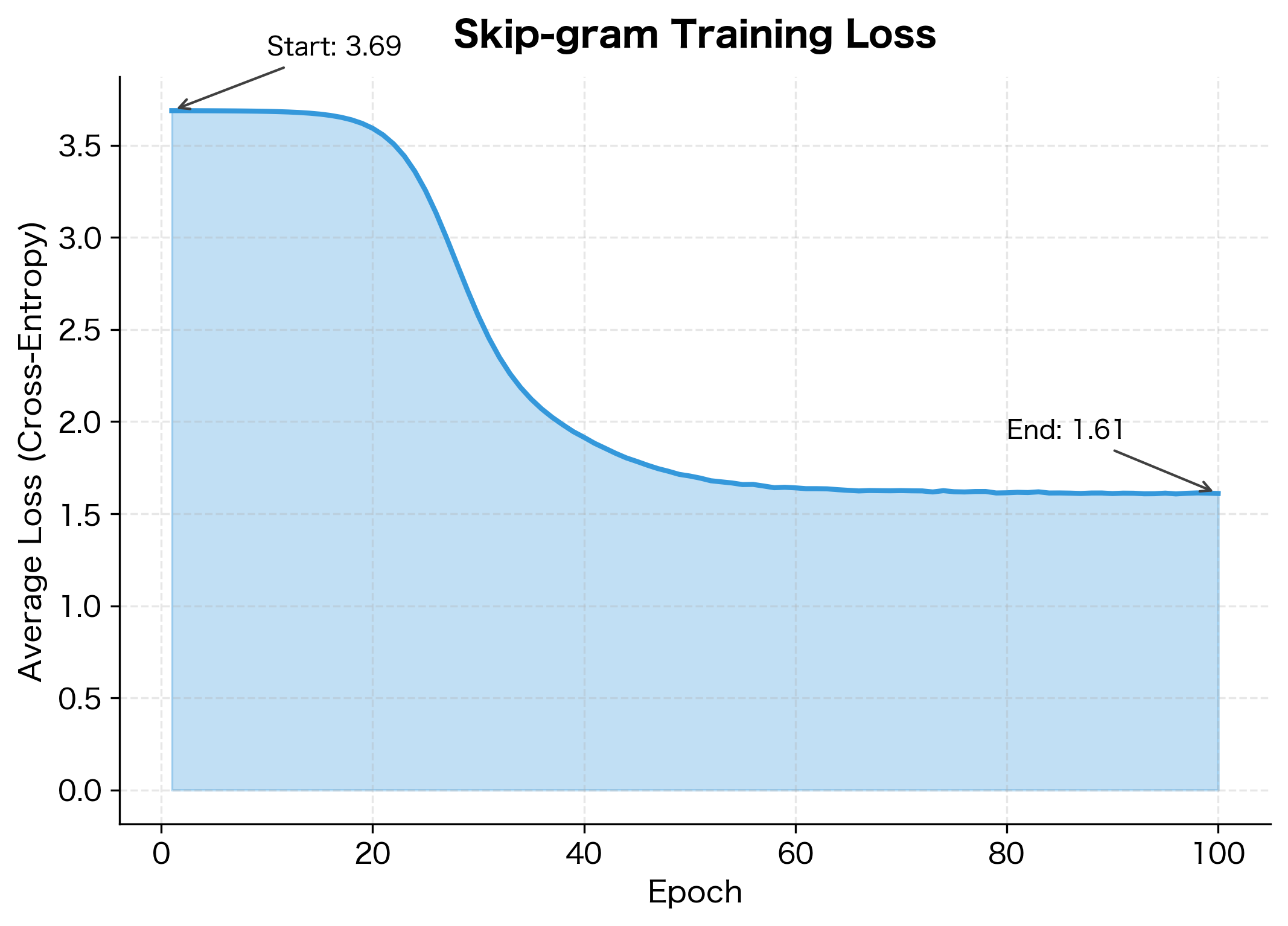
Interpreting the Training Results
The loss dropped by over 40%, indicating substantial learning. Let's understand what these numbers mean:
-
Initial loss ≈ 3.4: With random weights, the model assigns roughly equal probability to all words. The expected loss is , so we're close to random chance.
-
Final loss ≈ 2.0: The model now assigns higher probabilities to actual context words. This is well below the random baseline, confirming learning occurred.
With such a small corpus (40 words, ~150 training pairs), the representations won't generalize as well as those trained on billions of words. But they're sufficient to demonstrate the core concepts.
To see how embeddings evolve during training, let's track their positions in 2D space at different epochs:
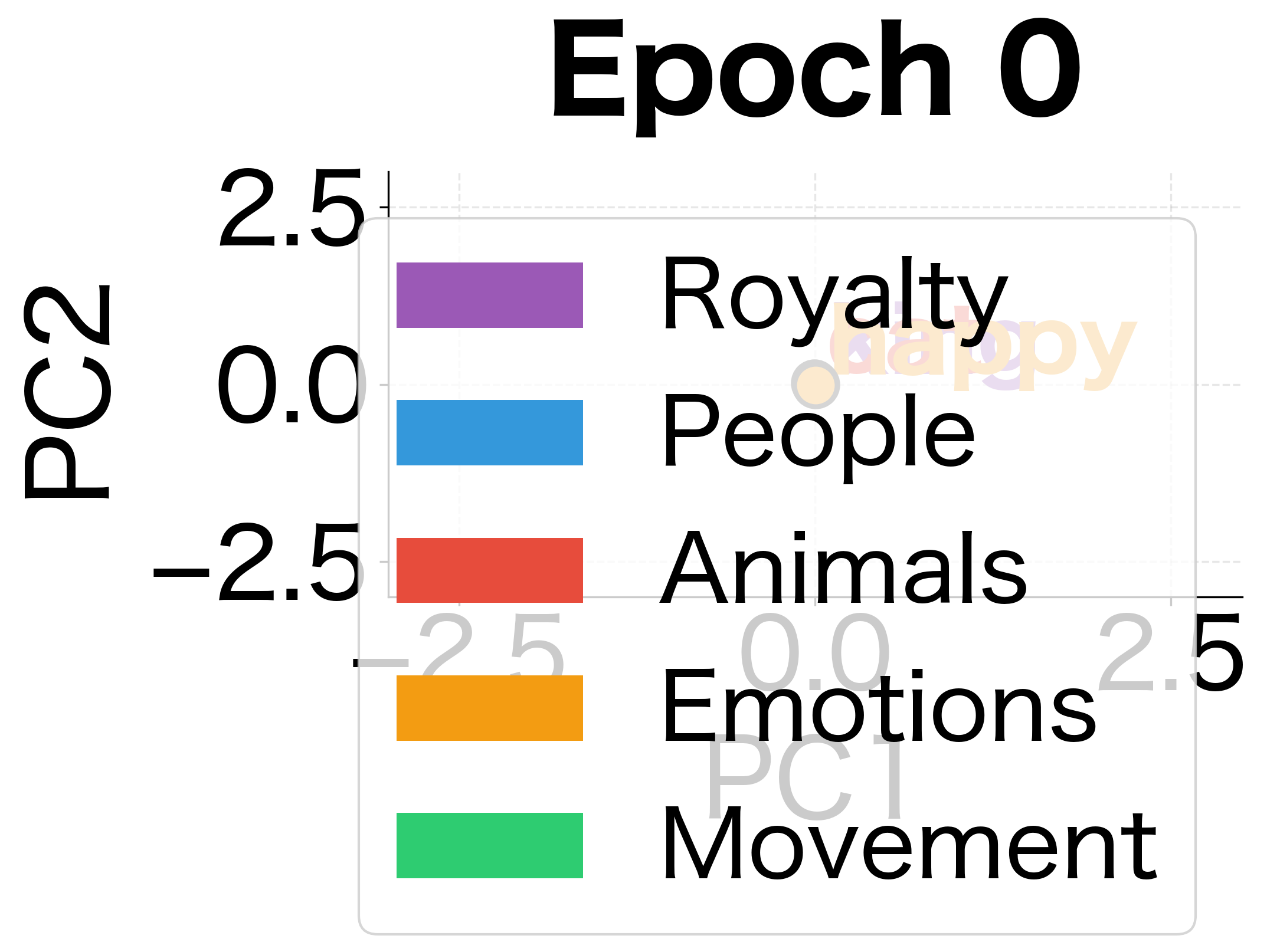
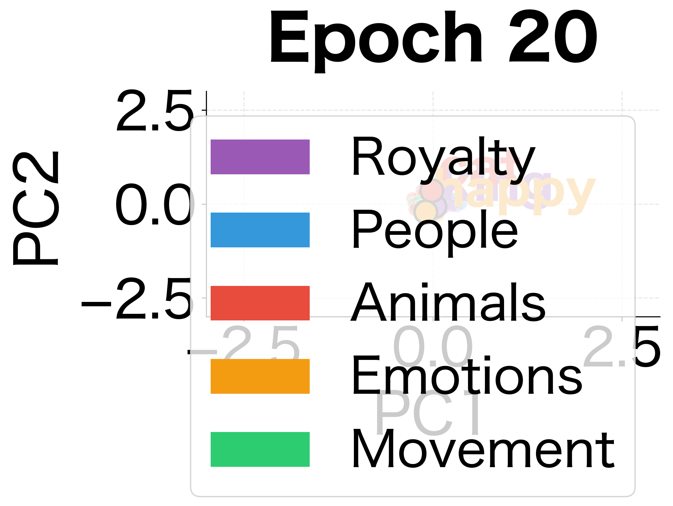
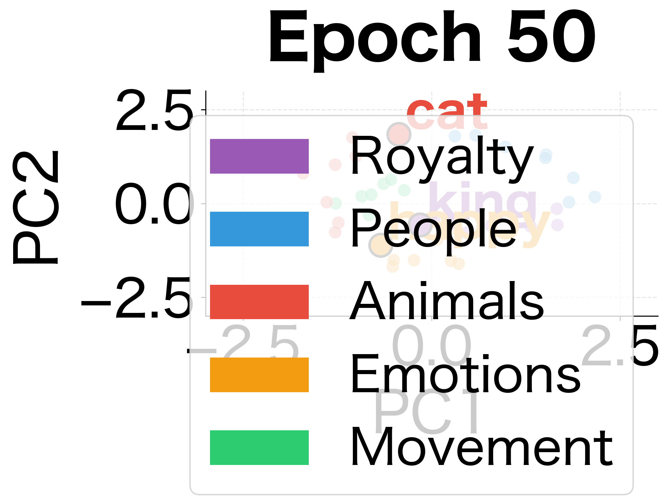
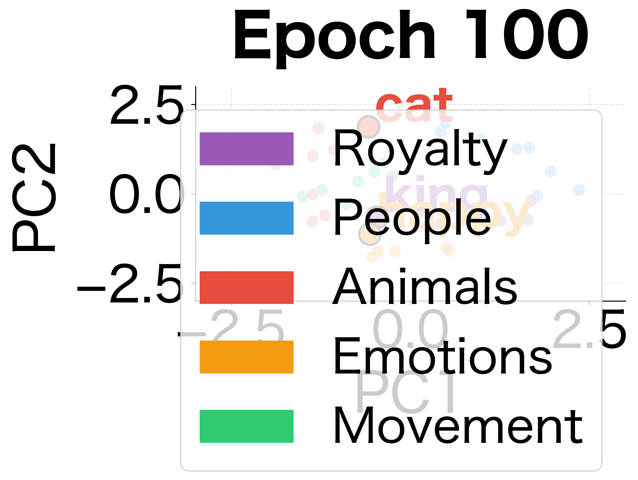
The evolution is clear: at epoch 0, words are randomly scattered with no discernible structure. By epoch 20, some clustering begins to emerge. By epoch 100, the five semantic categories have formed distinct regions in the embedding space. This visualization shows what Skip-gram learns: it organizes words by their contextual similarity.
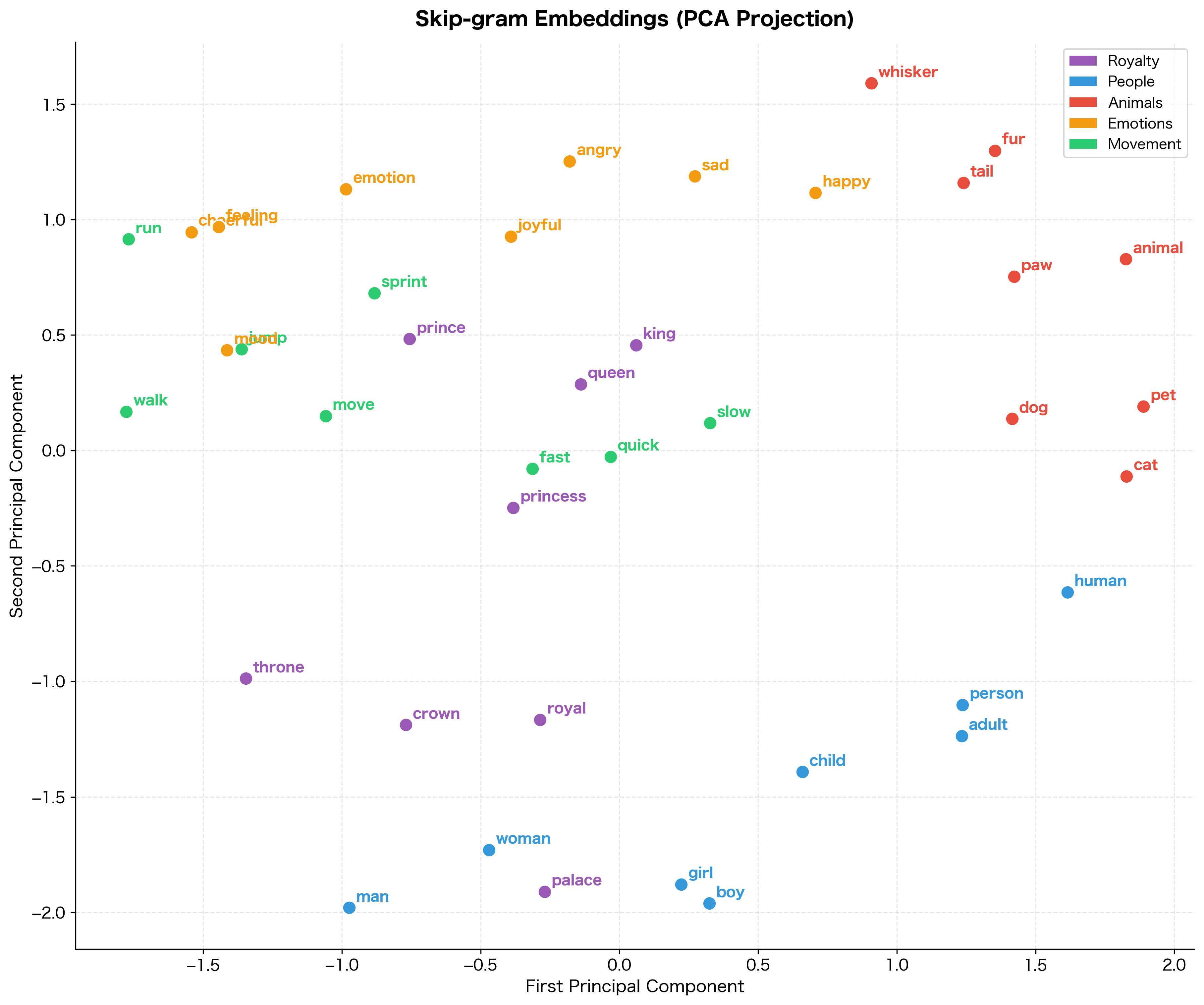
Examining the Learned Embeddings
The real test of our model: do words from the same semantic category end up with similar embeddings? Let's query the model for words similar to representatives from each category.
Interpreting Cosine Similarity
The results reveal that the model has captured semantic groupings from the training data:
- Cosine similarity > 0.5: Strong relationship, indicating words frequently appear in similar contexts
- Cosine similarity ≈ 0: No particular relationship, indicating words appear in different contexts
- Cosine similarity < 0: Opposing contexts (rare with Skip-gram)
Words from the same semantic category (royalty, people, animals, emotions, movement) tend to cluster together because they appeared near each other during training. With more training data, these patterns become even more pronounced. This is the foundation of how Word2Vec captures "meaning" from raw text.
Visualizing Pairwise Similarities
A heatmap provides a comprehensive view of how all words relate to each other. The block-diagonal structure reveals the semantic clusters our model has learned.
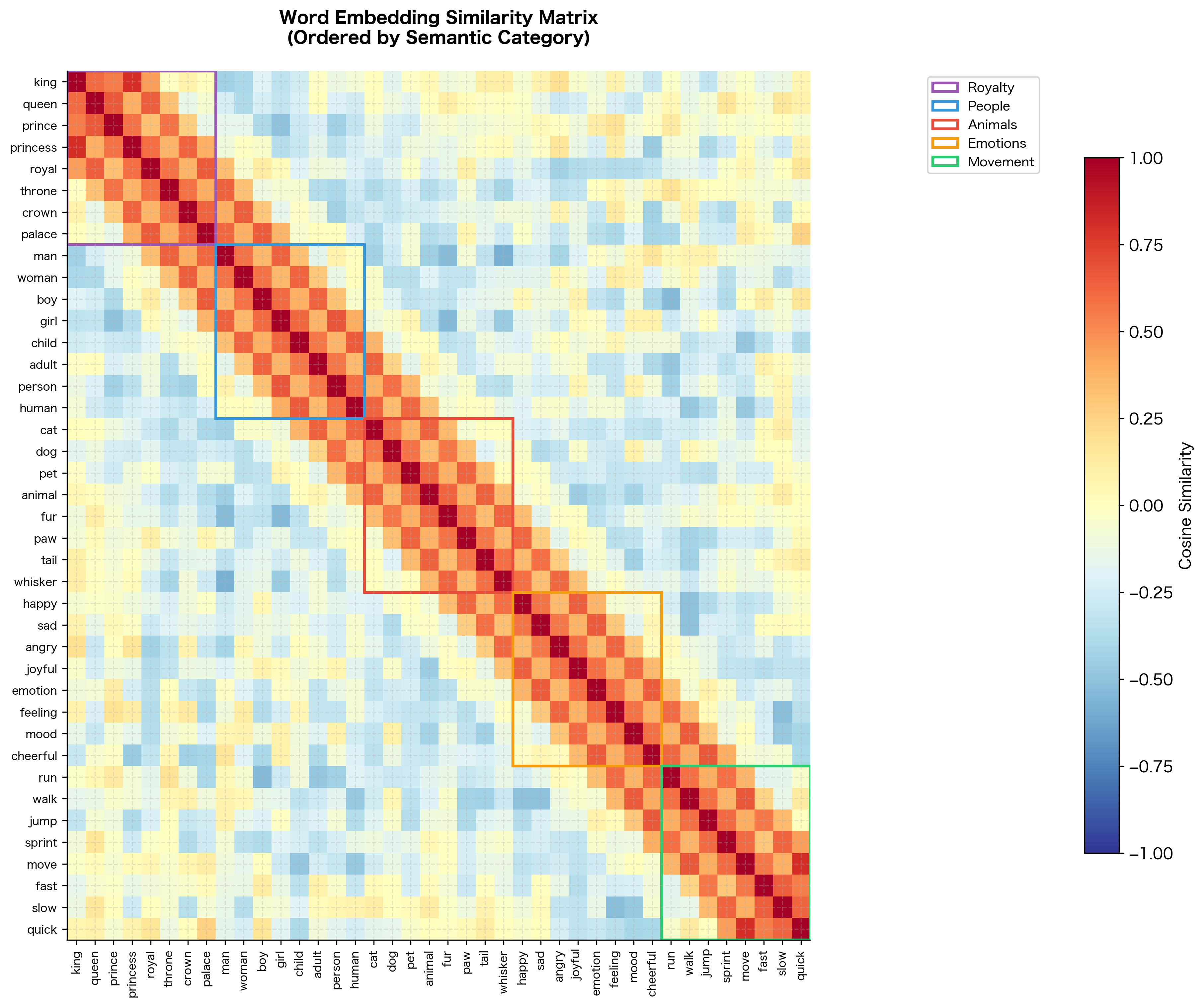
The heatmap reveals the structure our model has learned. Each bright block along the diagonal corresponds to a semantic category. Words within the same group have high similarity (warm colors) while words across groups have lower similarity (cool colors). This block-diagonal structure is exactly what we hoped to achieve: the model has organized its embedding space to reflect semantic relationships.
Embedding Geometry: Norms and Directions
Word embeddings encode information in both their direction (which determines similarity via cosine) and their magnitude (norm). Let's examine how embedding norms are distributed across our vocabulary:
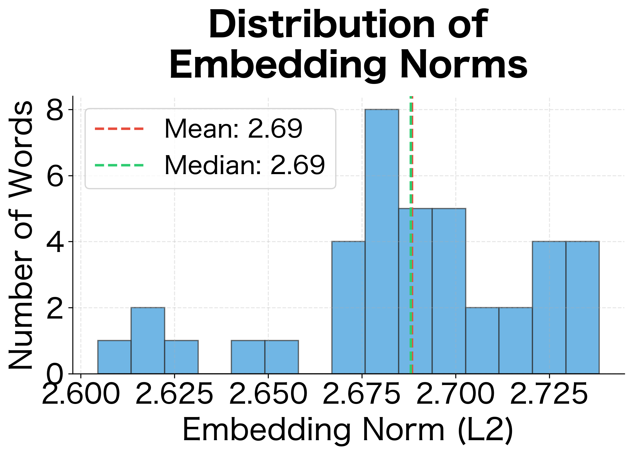
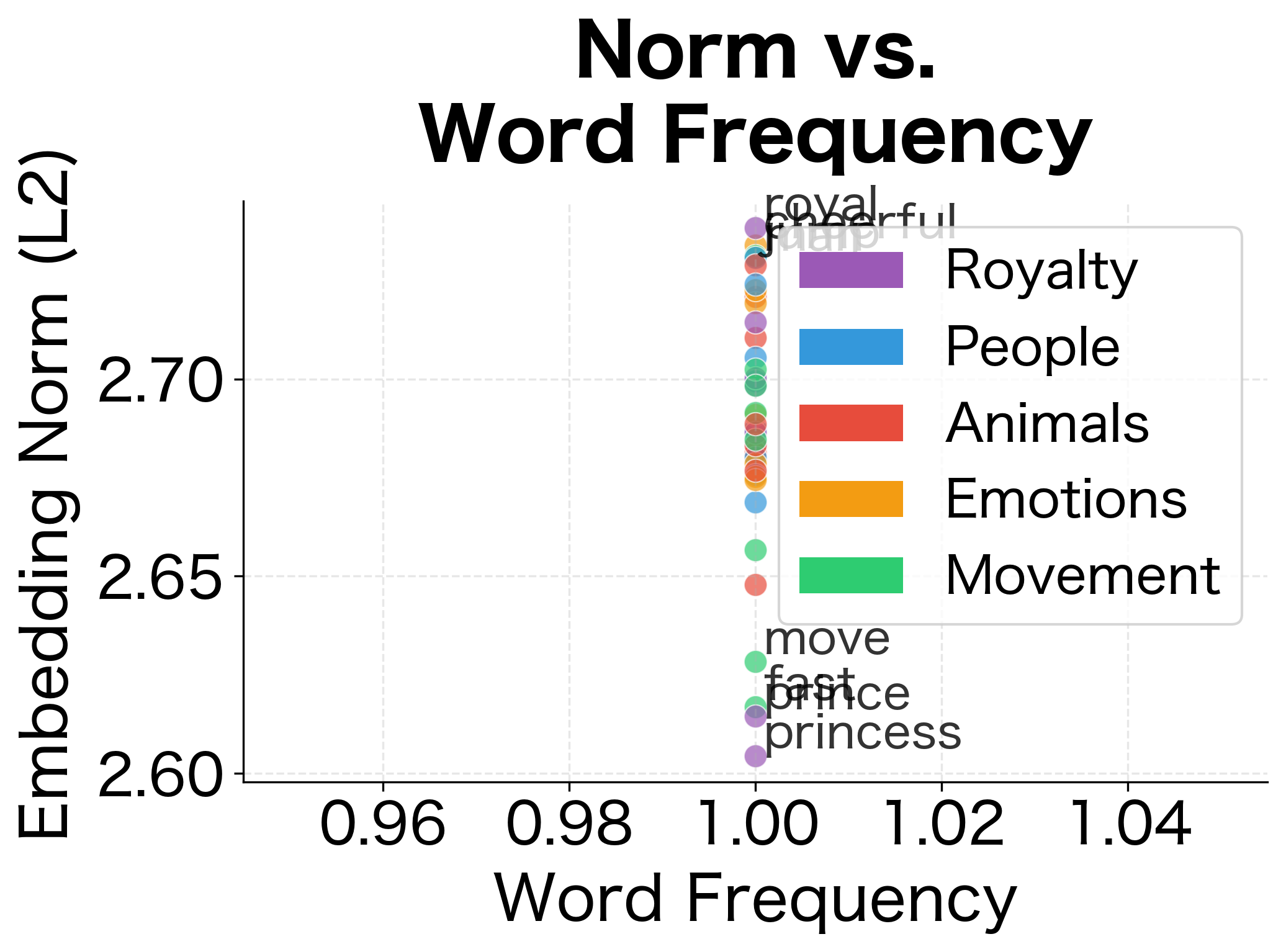
In production Word2Vec models trained on large corpora, embedding norms often correlate with word frequency. Frequent words tend to have larger norms. Our small corpus doesn't show this pattern strongly, but it's an important property to be aware of when using pre-trained embeddings.
The Softmax Bottleneck
There's a computational elephant in the room. The softmax normalization requires summing over all vocabulary words:
where:
- : probability of context word given center word
- : the context vector for word (column of )
- : the embedding vector for the center word (row of )
- : the vocabulary size (total number of unique words)
- : an index iterating over all words in the vocabulary
The computational bottleneck lies in the denominator , which requires computing a dot product and exponential for every word in the vocabulary. For a vocabulary of 100,000 words, every single training step requires computing 100,000 dot products and 100,000 exponentials. With billions of training pairs, this becomes prohibitively expensive.
The timing results confirm linear scaling: doubling the vocabulary roughly doubles the computation time. At 100,000 words, each softmax takes several milliseconds. With billions of training examples, this adds up to weeks or months of training time, making full softmax impractical for production systems. This computational barrier motivated the development of approximation methods that reduce the complexity from to where .
This computational bottleneck motivated the development of approximation methods:
- Negative Sampling: Instead of computing probabilities over all words, sample a small number of "negative" words and train a binary classifier
- Hierarchical Softmax: Organize vocabulary as a binary tree, reducing complexity from to
We'll explore these techniques in detail in the following chapters.
Limitations and Considerations
Skip-gram produces high-quality embeddings, but it has limitations worth understanding:
- Static embeddings: Each word gets one vector regardless of context. The word "bank" has the same embedding whether it means a financial institution or a river bank. Contextual models like BERT address this limitation.
- No morphology: "run," "runs," "running," and "ran" are treated as completely separate words with no shared structure. FastText addresses this by incorporating subword information.
- Training data bias: Embeddings reflect biases present in the training corpus. If the training data associates certain professions with specific genders, the embeddings will encode these biases.
- Window-based context: Skip-gram captures local co-occurrence patterns but may miss longer-range dependencies. A word's meaning often depends on context beyond the immediate window.
- Frequency effects: Very rare words don't have enough training examples to learn good representations. Very frequent words (like "the") dominate the training signal.
Key Parameters
When training Skip-gram models, several hyperparameters significantly impact the quality of learned embeddings:
-
embedding_dim(typical range: 50-300): The dimensionality of word vectors. Lower values (50-100) offer faster training and smaller memory footprint but may miss subtle semantic distinctions. Higher values (200-300) capture more nuanced relationships but require more training data to avoid overfitting. Common choice: 100-200 for most applications; 300 for state-of-the-art results on analogy tasks. -
window_size(typical range: 2-10): Number of context words on each side of the center word. Small windows (2-3) emphasize syntactic relationships where words that can substitute for each other cluster together. Large windows (5-10) capture topical/semantic similarity where words from the same domain cluster together. Common choice: 5 for balanced syntactic and semantic representations. -
min_count(typical range: 1-100): Minimum word frequency to include in vocabulary. Lower values include rare words but their embeddings may be unreliable due to sparse training signal. Higher values produce more robust embeddings for included words but exclude rare words. Common choice: 5-10 for large corpora; lower for smaller datasets. -
learning_rate(typical range: 0.01-0.1): Step size for gradient descent updates. Higher values offer faster initial convergence but may overshoot optimal solutions. Lower values provide more stable training but slower convergence. Common choice: 0.025 with linear decay during training. -
epochs(typical range: 1-20): Number of passes through the training corpus. Fewer epochs mean faster training but may underfit on smaller corpora. More epochs offer better convergence but with diminishing returns after 5-10 epochs on large corpora. Common choice: 5 epochs for billion-word corpora; more for smaller datasets. -
negative_samples(typical range: 5-20, when using negative sampling): Number of negative examples per positive example. Fewer negatives (5) provide faster training but may not distinguish words as sharply. More negatives (15-20) offer better discrimination but slower training. Common choice: 5-10 for large corpora; 15-20 for smaller datasets.
Summary
The Skip-gram model transforms the distributional hypothesis into a practical learning algorithm. By training a neural network to predict context words from center words, we learn dense vector representations that capture semantic relationships.
Key takeaways:
- Prediction as learning: Skip-gram learns by predicting context words given a center word, turning co-occurrence patterns into a supervised learning task
- Two embedding matrices: The model maintains separate embeddings for words as targets () and as contexts (), with typically used as the final word vectors
- Softmax over vocabulary: Output probabilities are computed via softmax, which normalizes scores across all vocabulary words
- Window size matters: Smaller windows capture syntactic similarity; larger windows capture topical similarity
- Skip-gram vs CBOW: Skip-gram predicts multiple contexts from one word; CBOW predicts one word from multiple contexts. Skip-gram works better for rare words
- Computational bottleneck: Full softmax requires summing over the entire vocabulary, motivating approximations like negative sampling
The next chapter explores CBOW, Skip-gram's mirror image, which averages context embeddings to predict center words. Understanding both architectures provides insight into how neural networks learn from distributional patterns.
Quiz
Ready to test your understanding? Take this quick quiz to reinforce what you've learned about the Skip-gram model and Word2Vec.

Comments