

A comprehensive guide to the Continuous Bag of Words (CBOW) model from Word2Vec, covering context averaging, architecture, objective function, gradient derivation, and comparison with Skip-gram.

This article is part of the free-to-read Language AI Handbook
Choose your expertise level to adjust how many terms are explained. Beginners see more tooltips, experts see fewer to maintain reading flow. Hover over underlined terms for instant definitions.
CBOW Model
In the previous chapter, we explored Skip-gram, which learns word embeddings by predicting context words from a center word. The Continuous Bag of Words (CBOW) model takes the opposite approach: given the surrounding context words, predict the center word. This architectural inversion leads to different learning dynamics and computational trade-offs.
CBOW was introduced alongside Skip-gram in the original Word2Vec paper by Mikolov et al. (2013). While Skip-gram treats each context position independently, CBOW averages context word embeddings together to make a single prediction per training example. This design choice has practical implications: CBOW trains faster than Skip-gram and performs better on frequent words, while Skip-gram excels at representing rare words.
This chapter covers the CBOW architecture from the ground up. We'll work through the mathematics, implement the model from scratch, and understand when to choose CBOW over Skip-gram.
The Core Idea: Predicting Words from Context
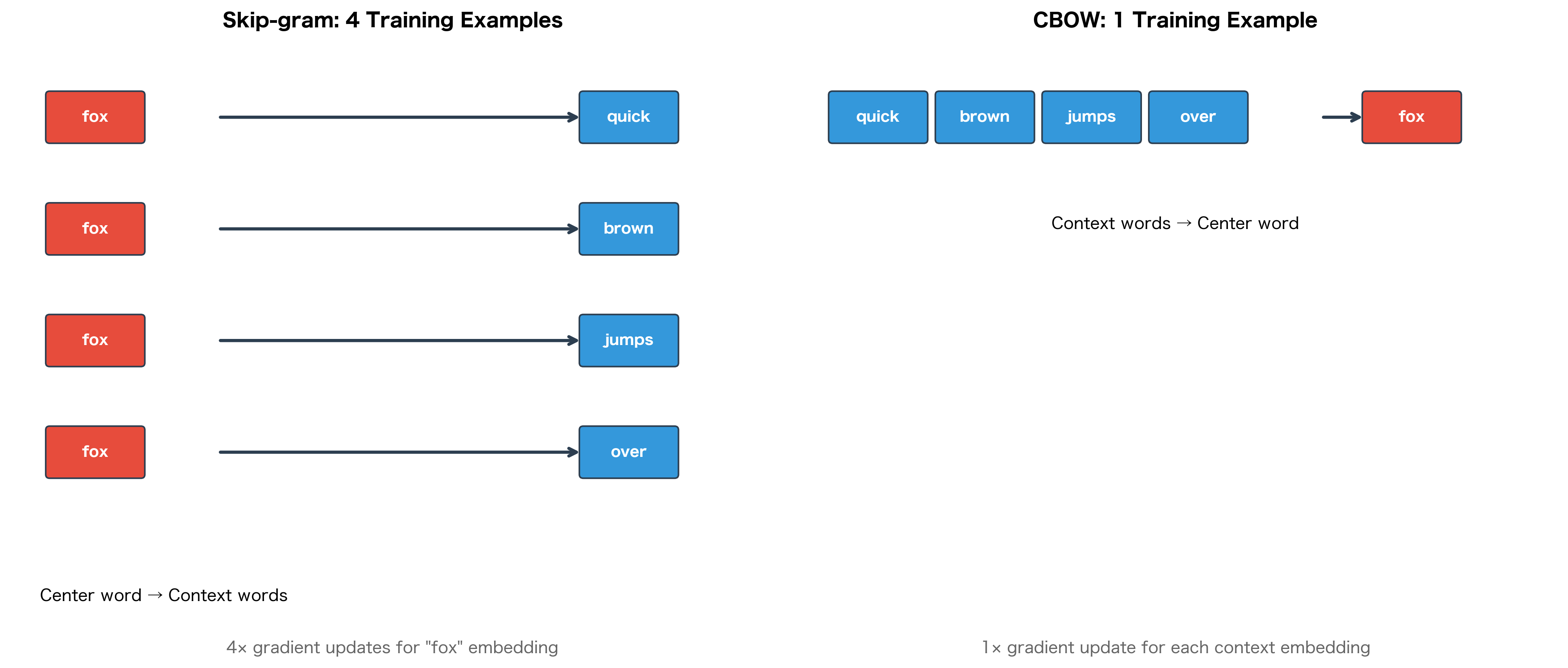
Imagine reading a sentence with a word missing: "The quick brown ___ jumps over the lazy dog." Given the surrounding context ("quick," "brown," "jumps," "over"), you can likely guess the missing word is "fox." This fill-in-the-blank task is exactly what CBOW learns to do.
The Continuous Bag of Words (CBOW) model learns word representations by training a neural network to predict a center word given its surrounding context words. The context word embeddings are averaged together before making the prediction.
The name "Continuous Bag of Words" comes from two properties:
- Continuous: The model uses continuous-valued vectors (embeddings) rather than discrete word representations
- Bag of Words: The context words are treated as an unordered set, averaging their embeddings together regardless of position
This single training example captures the essence of CBOW: given the surrounding words, predict what goes in the middle. Compare this to Skip-gram, which generates four separate training pairs from the same position: (fox → quick), (fox → brown), (fox → jumps), and (fox → over). CBOW instead creates one training example where all four context words together predict "fox."
Architecture: Context Averaging
CBOW's architecture is similar to Skip-gram but with a crucial difference in the input layer. Instead of taking a single word as input, CBOW takes multiple context words and averages their embeddings.
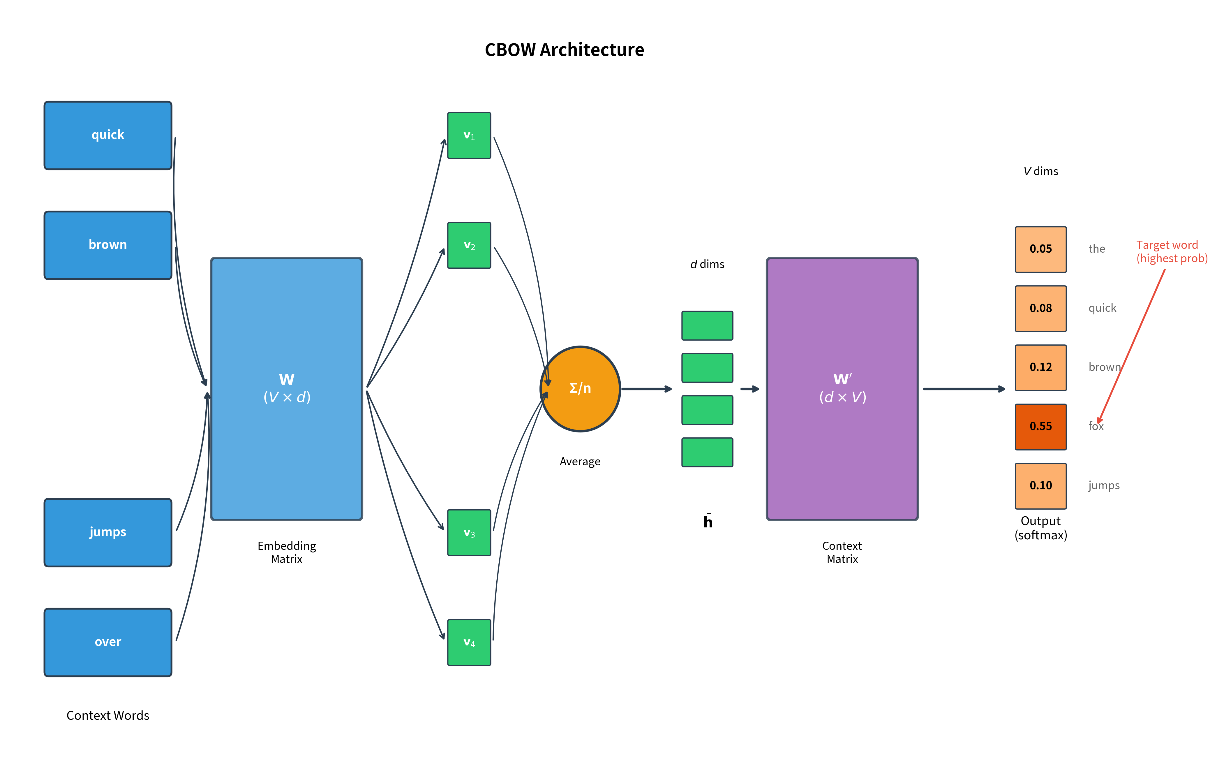
The network has two weight matrices, identical in purpose to Skip-gram:
-
Embedding matrix (size ): Maps input words to dense vectors. Each row is the embedding for one vocabulary word. For CBOW, we look up multiple rows (one per context word) and average them.
-
Context matrix (size ): Maps the hidden representation to output scores over the vocabulary.
The key difference from Skip-gram is what happens between the embedding lookup and the output layer: CBOW averages the context embeddings, while Skip-gram uses the single center word embedding directly.
Context Word Averaging
How should a model combine information from multiple context words? Skip-gram sidesteps this question entirely, processing each context word independently. But CBOW must somehow merge four separate embeddings into a single representation that captures the collective meaning of the context.
The simplest approach is also highly effective: take the average. If each context word embedding captures something about that word's meaning, then their average should capture what these words have in common. When the context words are semantically coherent (as they typically are around a meaningful center word), this average points toward the semantic region where the center word belongs.
This leads us to the core formula of CBOW. Given context words, the model computes their centroid in embedding space by taking the element-wise mean of their embedding vectors:
where:
- : the averaged hidden representation (a -dimensional vector representing the "centroid" of the context)
- : the number of context words (typically for a symmetric window of size on each side)
- : the -dimensional embedding vector of the -th context word (row of the embedding matrix )
- : summation over all context word embeddings
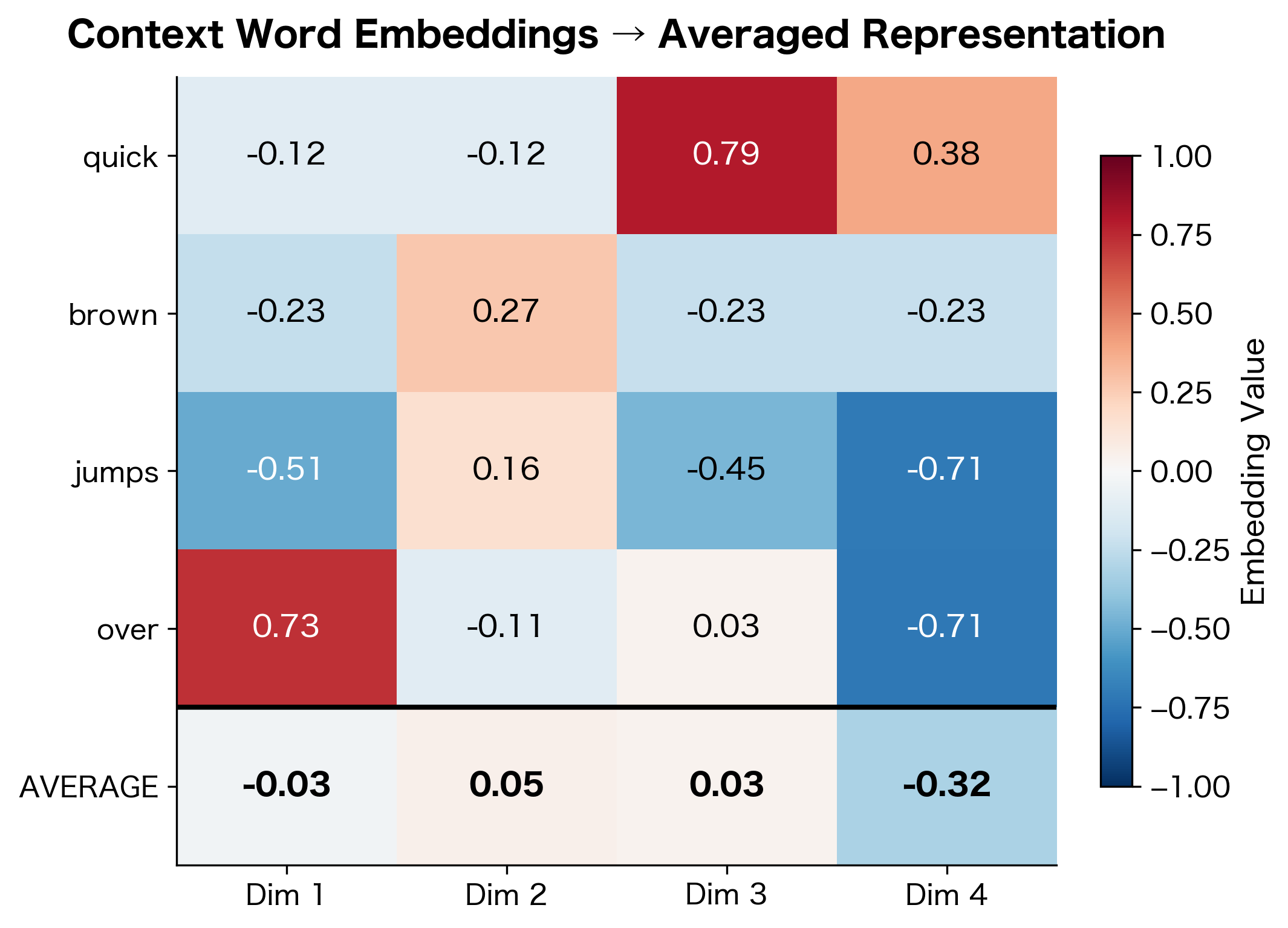
The averaging operation is simple: for each dimension of the embedding, . This element-wise mean produces values that lie between the extremes of the component vectors, smoothing out individual word idiosyncrasies while preserving shared semantic content.
This simplicity carries important implications for what CBOW can and cannot learn.
Each dimension of the averaged embedding is simply the mean of the corresponding dimensions from the individual word embeddings. Notice how the averaged vector smooths out the individual variations, producing values that lie between the extremes of the component vectors.
Averaging treats context words as an unordered set, a "bag of words." This simplification ignores word order (e.g., "dog bites man" averages the same as "man bites dog"), but works surprisingly well in practice. The key insight is that the set of nearby words, regardless of order, provides strong signal about a word's meaning.
Visualizing Context Averaging
Let's visualize how averaging combines multiple context vectors into a single representation:
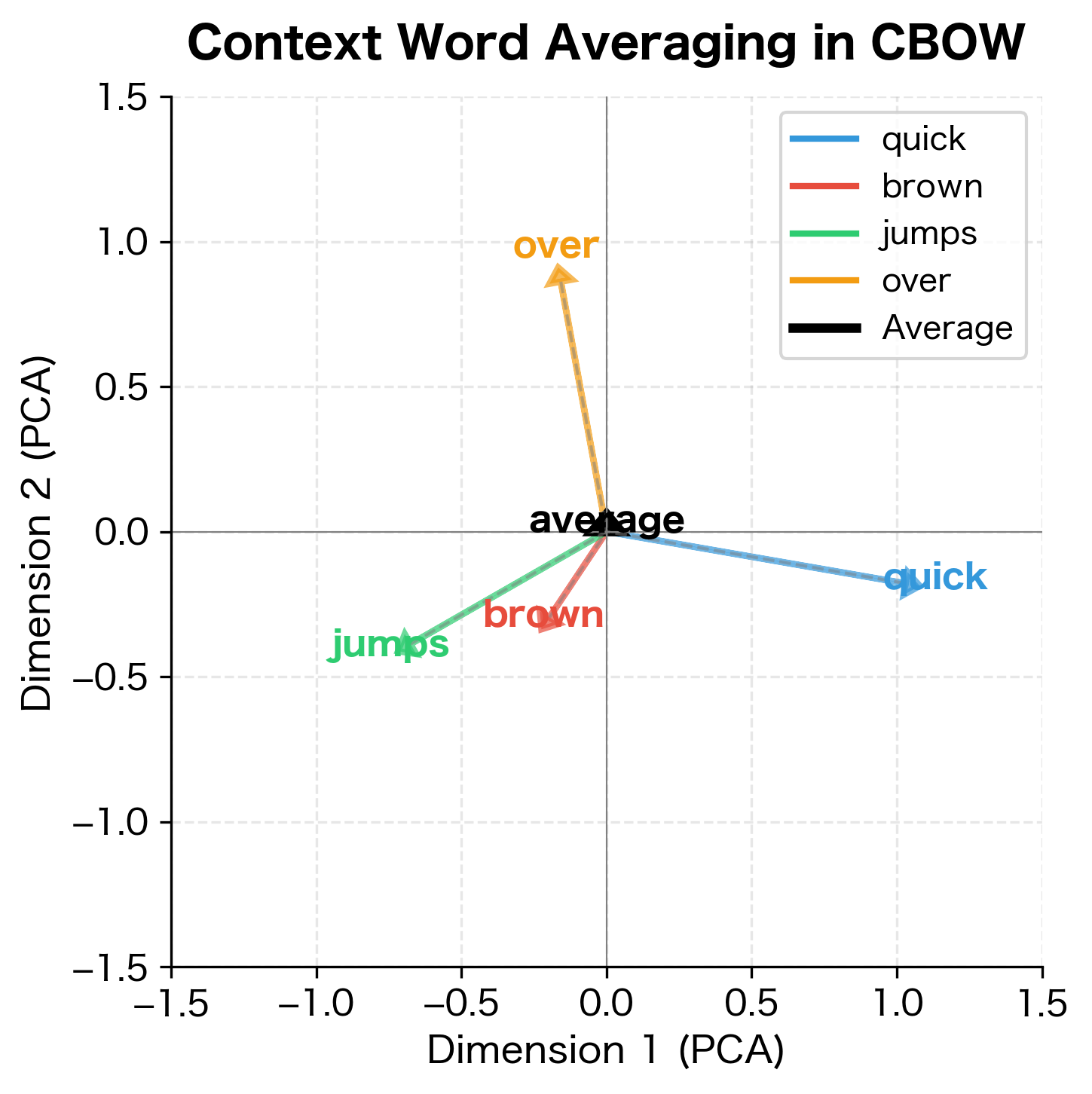
The averaged vector represents the semantic centroid of the context. When context words are semantically coherent (as they typically are around a meaningful center word), this centroid points toward the region of embedding space where the center word should reside.
The CBOW Objective Function
With the averaged context representation in hand, CBOW faces a classification problem: which of the vocabulary words is most likely to appear in the center position? This is where the second weight matrix, , comes into play.
From Context to Prediction
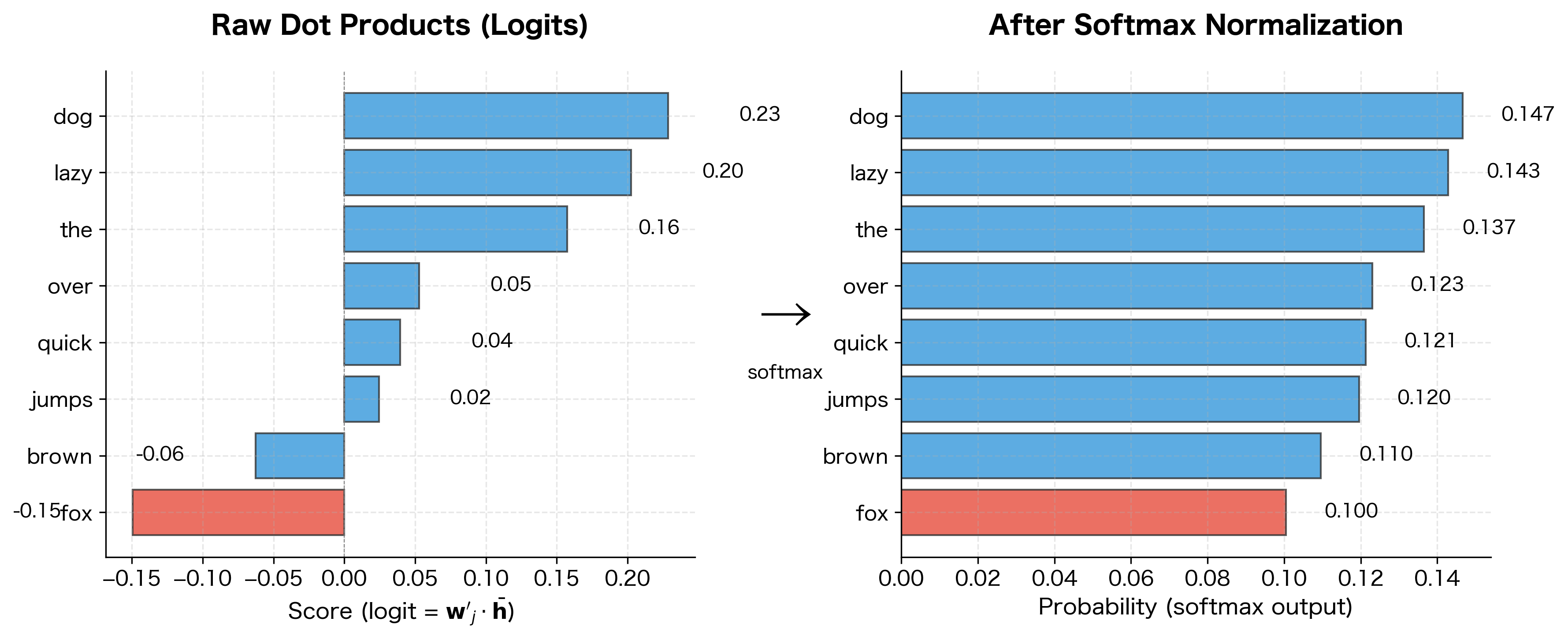
The intuition behind the prediction step is geometric. Each word in the vocabulary has a corresponding vector in the context matrix . To predict the center word, CBOW computes how well the averaged context aligns with each vocabulary word's context vector. The word whose context vector points most in the same direction as receives the highest probability.
This alignment is measured by the dot product. For the target word , we compute , which yields a large positive value when the vectors point in similar directions. But we need probabilities, not raw scores, so we apply softmax normalization.
The softmax function converts a vector of real-valued scores into a probability distribution. Applied to our word prediction task, it computes:
where:
- : the probability of word being the center word, given context words
- : the target center word we're trying to predict
- : the averaged context embedding (computed from the input layer)
- : the context vector for word (column of )
- : the exponential of the dot product, ensuring the numerator is always positive
- : the normalization constant, summing over all vocabulary words to ensure probabilities sum to 1
- : vocabulary size (total number of words in the vocabulary)
The exponential function serves two purposes: (1) it maps any real-valued dot product to a positive number, ensuring valid probabilities, and (2) it amplifies differences between scores, so words with higher dot products receive exponentially higher probability mass. The denominator normalizes these values so they sum to 1 across the vocabulary.
This is the same formulation as Skip-gram, but with the averaged context vector replacing the single center word embedding.
From Probability to Loss
Training requires a loss function that measures prediction quality. The natural choice is cross-entropy loss, which penalizes the model for assigning low probability to the correct center word.
Starting from the probability formula, we take the negative logarithm to obtain the loss:
Step 1: Begin with the softmax probability for the target word:
Step 2: Apply the negative log to convert to a loss (lower probability → higher loss):
Step 3: Apply the logarithm quotient rule, :
Step 4: Simplify using :
where:
- : the cross-entropy loss for a single training example (a non-negative scalar)
- : the dot product (alignment score) between the target word's context vector and the averaged context embedding
- : the "log-sum-exp" normalization term
This loss has an intuitive interpretation. The first term, , wants to maximize the dot product between the context representation and the correct word, pushing them to align in embedding space. The second term, the log-sum-exp, acts as a normalizing penalty that prevents all dot products from growing unboundedly large. Without this term, the model could trivially reduce loss by scaling all vectors to infinity.
The Corpus Objective
The loss applies to a single training example. For a complete training corpus, we aggregate the losses over all word positions by computing their average:
where:
- : the corpus-level objective function (average loss across the entire corpus)
- : the total number of training positions in the corpus (each position where we extract a center word and its context)
- : the cross-entropy loss at position (computed using the formula derived above)
- : summation over all training positions
Minimizing this objective encourages the model to correctly predict center words from their contexts across the entire corpus. During training, we use stochastic gradient descent to update the embedding matrices and to reduce .
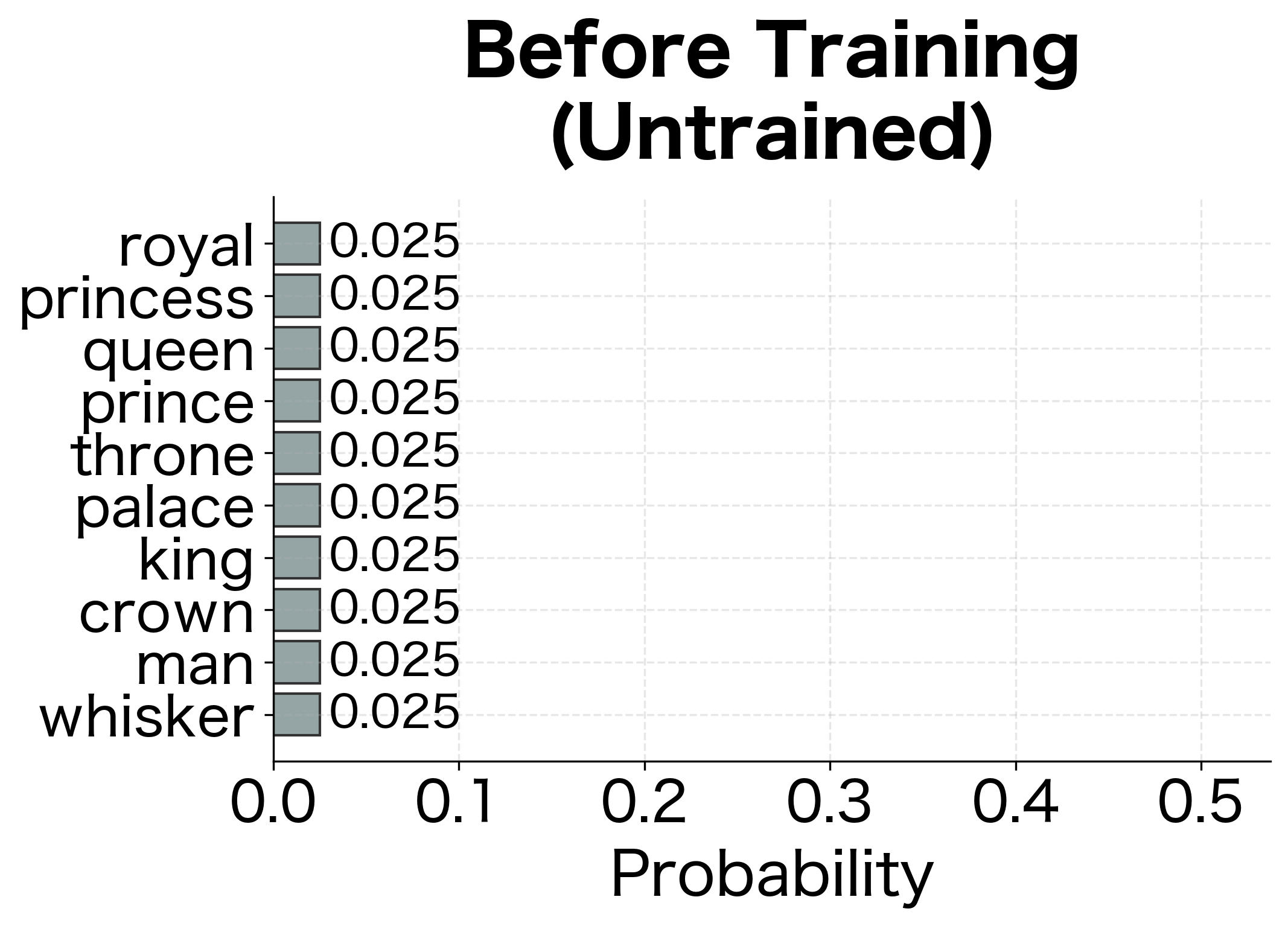
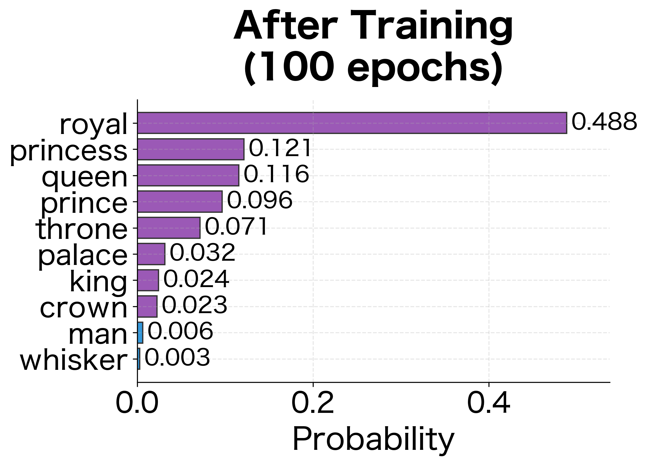
With random weights, the model has no preference for the correct word. Training adjusts the embeddings so that the averaged context vector produces high probability for the actual center word.
CBOW vs Skip-gram: A Detailed Comparison
While CBOW and Skip-gram share the same embedding matrices, they differ fundamentally in how they use training data.
Training Signal Density
Consider the sentence "The quick brown fox jumps over the lazy dog" with window size 2. At position 3 (word "fox"):
Skip-gram generates 4 training pairs:
- (fox → quick)
- (fox → brown)
- (fox → jumps)
- (fox → over)
Each pair updates the "fox" embedding based on predicting one context word.
CBOW generates 1 training example:
- (quick, brown, jumps, over → fox)
This single example updates all four context word embeddings based on predicting "fox."
Implications for Rare vs. Frequent Words
This difference in training structure has important consequences:
Rare words benefit more from Skip-gram:
- Each occurrence of a rare word in Skip-gram generates multiple training examples (one per context word)
- In CBOW, a rare word appearing as center word creates only one training example
- A rare word appearing in context contributes only a fraction (1/C) of the gradient
Frequent words can benefit from CBOW:
- CBOW's averaging smooths out noisy context patterns
- For frequent words with many training examples, the averaging helps learn stable representations
- The single prediction per position makes training faster
Table training-signal quantifies how Skip-gram provides proportionally more training signal per word occurrence.
| Word | Frequency | Skip-gram | CBOW | Ratio |
|---|---|---|---|---|
| "the" | 9 | 32 | 16.0 | 2.0× |
| "king" | 1 | 4 | 2.0 | 2.0× |
| "ceremony" | 1 | 4 | 2.0 | 2.0× |
Training Speed
CBOW is faster to train than Skip-gram for two reasons:
- Fewer forward/backward passes: CBOW makes one prediction per position; Skip-gram makes predictions
- Shared computation: The context averaging in CBOW reuses embeddings; Skip-gram computes independently
The benchmark confirms the theoretical speedup. CBOW processes each corpus position faster because it makes one prediction rather than multiple predictions. For corpora with billions of words, this speedup translates to hours or even days of saved training time.
Summary of Trade-offs
| Aspect | Skip-gram | CBOW |
|---|---|---|
| Training examples per position | (one per context word) | 1 (all context words together) |
| Training speed | Slower | Faster (3-4×) |
| Rare words | Better (more training signal) | Worse (diluted in average) |
| Frequent words | Good | Better (averaging smooths noise) |
| Memory usage | Same | Same |
| Final embedding quality | Slightly better overall | Competitive, especially for frequent words |
The Forward Pass
Let's implement the complete CBOW forward pass. Given context words, we compute the probability distribution over vocabulary words:
The untrained model assigns roughly uniform probabilities across vocabulary words, reflecting its lack of learned associations. After training, the model will concentrate probability mass on the actual center word.
Gradient Derivation
With the forward pass defined, we now derive the gradients needed to train CBOW. Understanding these gradients reveals why CBOW behaves differently from Skip-gram during training, particularly the crucial insight that context words share the gradient signal.
Recall the loss for a single training example:
Training requires computing how this loss changes with respect to each weight in the model. We'll work backward through the network, starting at the output and flowing gradients back to the input embeddings.
Gradient for the Context Matrix
The context matrix directly produces the output scores. Each column represents word in the output layer. To train the model, we need to compute how the loss changes when we adjust these vectors.
Step 1: Recall that the loss depends on through the term . For the target word , this appears in the numerator; for all words, it appears in the denominator.
Step 2: Taking the partial derivative of the loss with respect to for any word :
where:
- : the gradient of the loss with respect to the context vector for word (a -dimensional vector)
- : the indicator function, equal to 1 if (the target word), and 0 otherwise
- : the averaged context embedding
- The fraction is the softmax probability
The first term, , only appears for the target word. It pushes toward to increase the dot product (and thus the probability) for the correct answer. The second term pulls all words' context vectors away from in proportion to their predicted probability.
Step 3: Recognizing that the fraction is simply , we can simplify:
This elegant formula shows the gradient is proportional to the "prediction error":
- For the target word (): The gradient is . Since , this is negative, meaning we increase (push the vectors to align).
- For all other words (): The gradient is . This is positive, meaning we decrease (push the vectors apart).
Step 4: In matrix form, we can express this compactly using the outer product:
where:
- : the gradient matrix (size )
- : the averaged context embedding (size )
- : the outer product operation, producing a matrix from vectors of size and
- : the softmax output probability vector (size , with entries for each word)
- : the one-hot target vector (size , with 1 at position and 0 elsewhere)
- : the error vector, measuring how far each predicted probability is from the target
Gradient for the Embedding Matrix
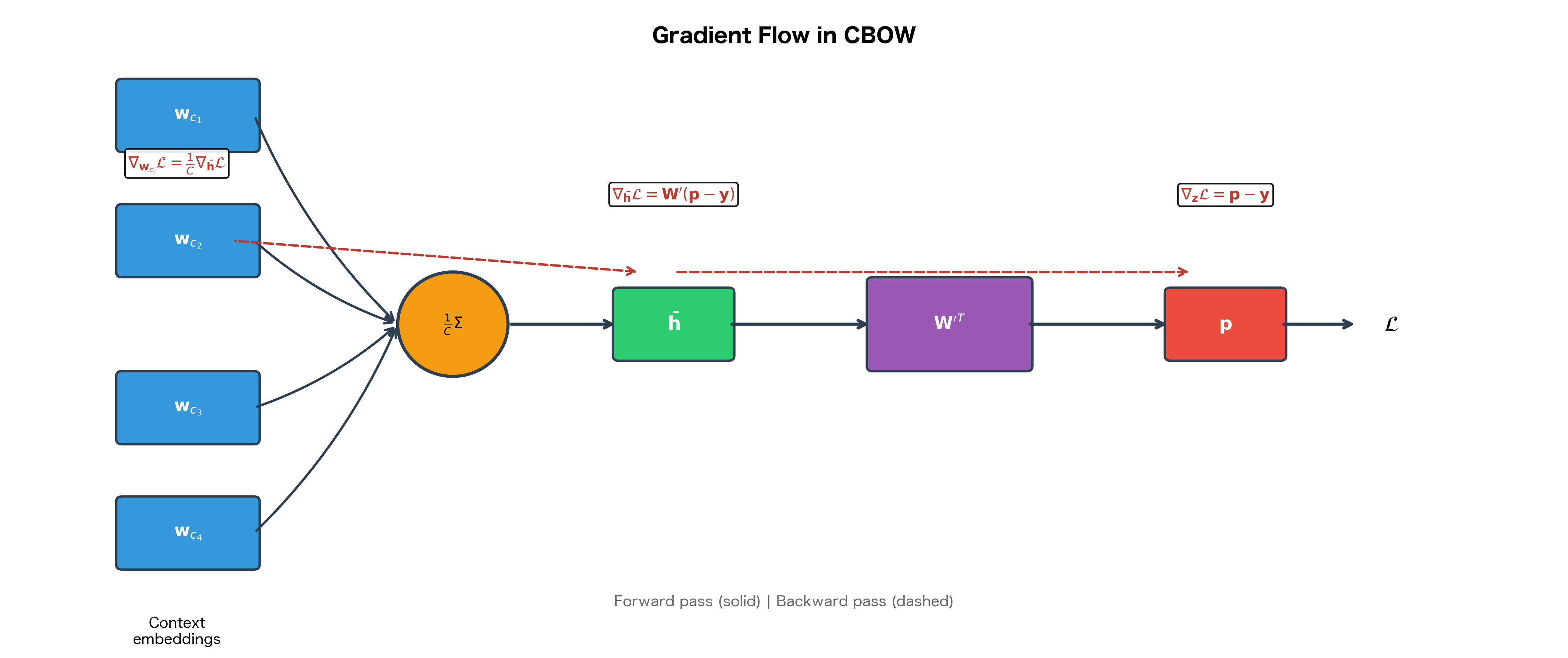
The gradient must flow backward through the averaging operation to reach the input embeddings. This is where CBOW fundamentally differs from Skip-gram.
Step 1: Compute the gradient with respect to the averaged representation . Using the chain rule, this requires multiplying by the context matrix:
where:
- : the gradient of the loss with respect to the averaged context vector (a -dimensional vector)
- : the context matrix (size )
- : the error vector (size )
- The matrix-vector product produces a -dimensional vector
This gradient tells us how the loss would change if we nudged in any direction. But is not a learnable parameter; it's computed as the average of the context word embeddings. We must therefore distribute this gradient to the actual parameters: the embedding vectors .
Step 2: Apply the chain rule to propagate the gradient through the averaging operation. Recall that:
Taking the partial derivative of with respect to any context word embedding :
Each context word contributes exactly to the average, so each receives of the gradient.
Step 3: Apply the chain rule to get the gradient for each context word embedding:
where:
- : the gradient for the -th context word embedding (a -dimensional vector)
- : the scaling factor from the averaging operation
- : the gradient at the averaged representation (computed in Step 1)
Each context word embedding receives exactly of the gradient signal. This division has important implications:
-
Diluted learning for rare words: A rare word appearing in a context of four words receives only 25% of the gradient that a center word would receive in Skip-gram.
-
Smoothed updates: The averaging acts as implicit regularization, preventing any single context word from dominating the update.
-
Faster training: Despite the dilution, CBOW processes each corpus position with a single forward-backward pass, making it faster overall.
Complete Implementation with Training
The mathematical framework is now complete: we know how to compute predictions (forward pass) and how to compute gradients for learning (backward pass). Let's bring these pieces together into a working implementation.
The implementation follows the gradient equations exactly. In the backward pass, notice how the gradient first flows to through the context matrix, then divides by before reaching each context word embedding. This is the gradient division we derived earlier.
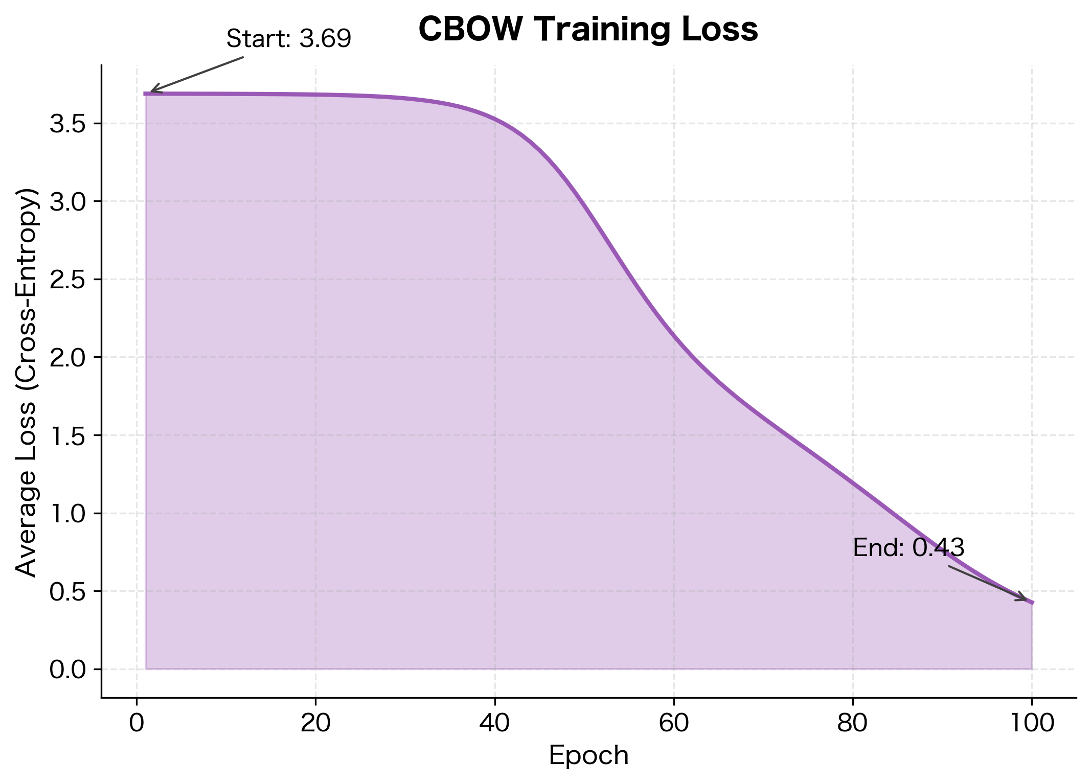
Training on a Toy Corpus
The loss reduction indicates the model has learned to predict center words from their context. The initial loss reflects random guessing across the vocabulary, while the final loss shows the model assigns higher probability to actual center words.
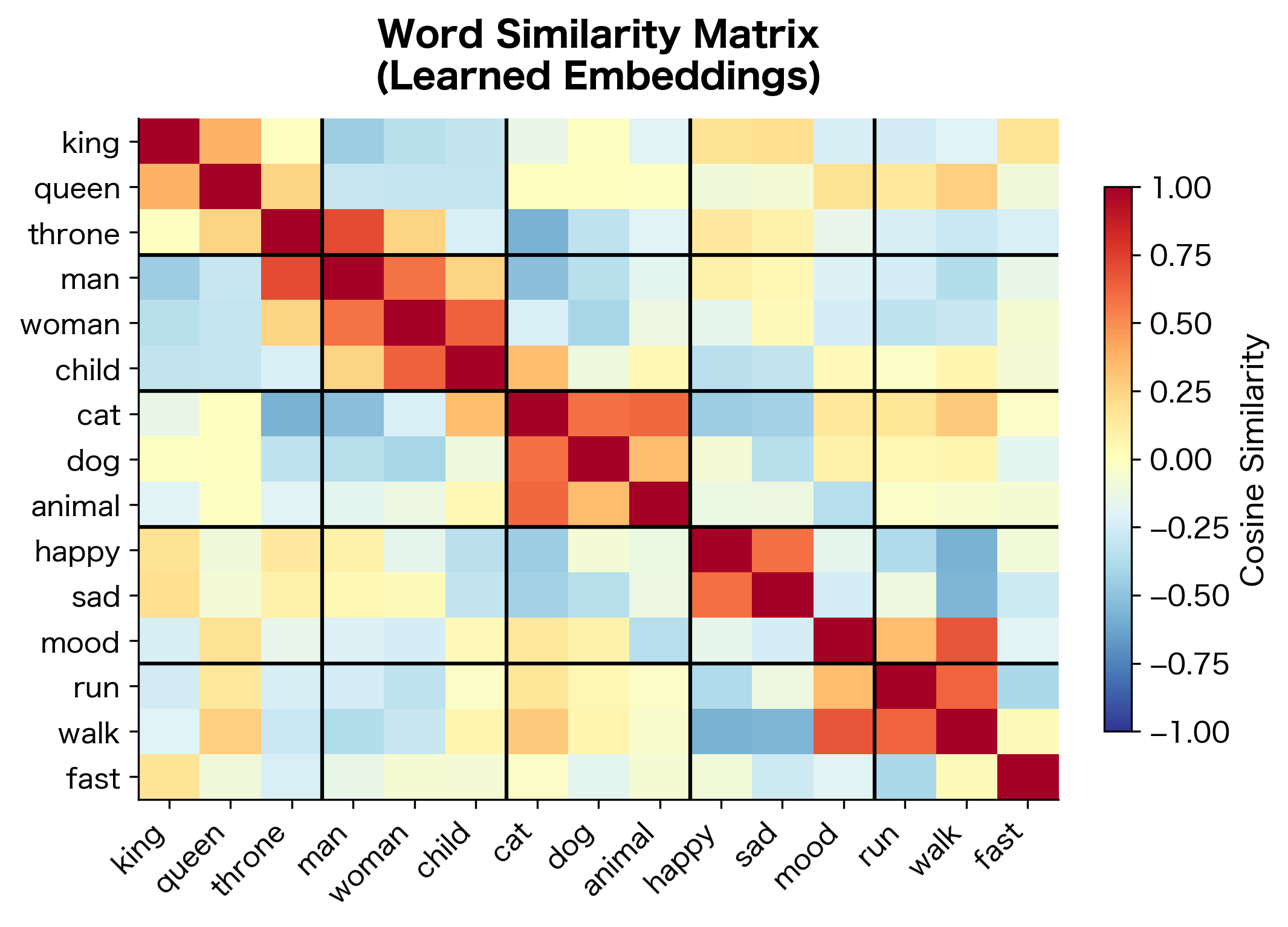
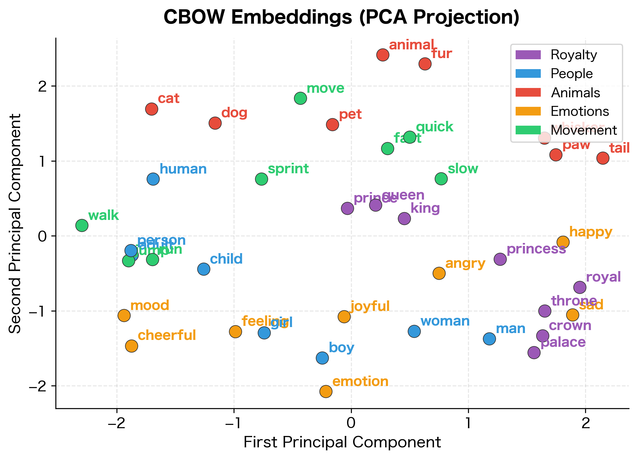
Examining Learned Embeddings
The model has learned that words appearing in similar contexts have similar embeddings. Words from the same semantic category cluster together in embedding space, demonstrating that CBOW successfully captures distributional semantics even on this small corpus.
When to Choose CBOW
Given the trade-offs between CBOW and Skip-gram, when should you reach for CBOW? The model excels in specific scenarios:
- Large corpora with common words: When you have billions of words and care most about representing frequent vocabulary, CBOW's faster training and averaging-based smoothing are advantageous.
- Time-constrained training: If computational resources are limited, CBOW's 3-4x speedup over Skip-gram can make training feasible where it otherwise wouldn't be.
- Syntactic tasks: Some research suggests CBOW performs slightly better on syntactic analogy tasks (e.g., "big : bigger :: small : ?"), possibly because averaging captures grammatical patterns effectively.
- Downstream averaging: If your application averages word embeddings to create sentence or document representations, CBOW's training objective aligns naturally with this use case.
Limitations of Context Averaging
While CBOW's averaging approach enables faster training and smoother representations, the bag-of-words assumption introduces inherent limitations that affect what the model can learn:
- Order insensitivity: "dog bites man" and "man bites dog" produce identical averaged context representations, even though they mean very different things.
- Dilution of rare context words: A rare but informative context word contributes only of the gradient, potentially getting drowned out by more common words in the same context window.
- Position blindness: A word immediately adjacent to the target is treated the same as a word at the edge of the window. Some extensions weight by distance to address this.
Position-Weighted Variants
The position blindness limitation motivates an extension to standard CBOW. In standard CBOW, all context words contribute equally to the averaged representation, regardless of their distance from the center word. However, words immediately adjacent to the target often carry more semantic relevance than words at the edge of the window.
Some implementations address this by weighting context words based on their distance from the target. Instead of a simple average, we compute a weighted average:
where:
- : the weighted averaged hidden representation (a -dimensional vector)
- : the number of context words in the window
- : the weight for the -th context word (typically decreasing with distance from center)
- : the embedding vector of the -th context word
- : the sum of all weights, used to normalize the weighted sum
The numerator computes a weighted sum of the context embeddings, and the denominator normalizes by the total weight. When all , this reduces to the standard averaging formula.
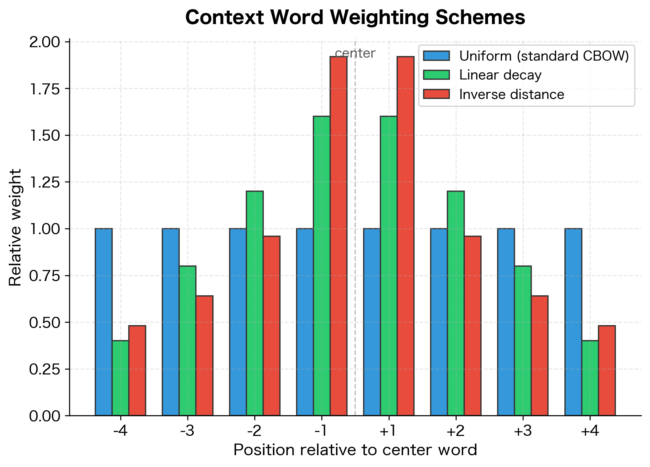
Common weighting schemes define based on the position offset (the signed distance from the center word):
- Linear decay: , where is the absolute distance from the center word and is the window size. This gives weight 1 to the closest words and linearly decreases to 0 at distance .
- Inverse distance: , where is the absolute distance. Words at position receive weight 1, words at receive weight 0.5, and so on.
- Exponential decay: , where is a hyperparameter controlling the decay rate. Larger values concentrate more weight on nearby words.
Implementing Position Weighting
Let's implement a weighted averaging function that supports different distance-based weighting schemes:
The different weighting schemes produce distinct averaged embeddings. With inverse distance weighting, the words at positions -1 and +1 (closest to the center) contribute more to the final representation than those at -2 and +2. This can improve embedding quality when nearby context words carry more semantic relevance than distant ones.
The Softmax Bottleneck (Again)
Like Skip-gram, CBOW faces the softmax computational bottleneck. Recall that each training step requires computing the probability for the target word:
where:
- : the probability of the target word given the context
- : the context vector for the target word (column of )
- : the averaged context embedding
- : the vocabulary size
- : the expensive summation over all vocabulary words
The computational bottleneck lies in the denominator. For each training step, we must:
- Compute dot products: for every word in the vocabulary
- Compute exponentials: for each word
- Sum all exponentials to get the normalization constant
For a vocabulary of 100,000 words, this means 100,000 dot products and exponentials per training step, a significant computational burden that scales linearly with vocabulary size, .
The same approximation techniques that accelerate Skip-gram also apply to CBOW:
- Negative sampling: Sample a small number of negative examples instead of computing the full softmax, reducing per-step complexity from to where
- Hierarchical softmax: Use a binary tree structure to reduce complexity from to
We'll cover these techniques in detail in subsequent chapters.
Key Takeaways
CBOW and Skip-gram are complementary approaches to learning word embeddings from context:
- Architectural difference: CBOW averages context embeddings to predict the center word; Skip-gram uses the center word to predict each context word
- Training dynamics: CBOW creates one training example per position, Skip-gram creates examples. CBOW is faster but provides less training signal for rare words
- Context averaging: The "bag of words" assumption treats context as an unordered set, losing word order information but capturing overall semantic context
- Gradient distribution: Each context word receives of the gradient, diluting the signal for any single word. This explains why rare words benefit more from Skip-gram
- Practical trade-offs: Choose CBOW when training speed matters and vocabulary is dominated by frequent words. Choose Skip-gram when rare word quality matters
The next chapter explores negative sampling, which accelerates both CBOW and Skip-gram by replacing the expensive softmax with a simpler binary classification objective.
Key Parameters
When training CBOW models, several hyperparameters impact embedding quality:
embedding_dim(typical range: 50-300): The dimensionality of word vectors. Lower values (50-100) provide faster training and smaller memory footprint, sufficient for many tasks. Higher values (200-300) capture more nuanced relationships but require more data. A common choice is 100-200 for most applications.window_size(typical range: 2-10): Number of context words on each side of the center word. Small windows (2-3) emphasize syntactic relationships, while large windows (5-10) capture broader topical similarity. A common choice is 5 for balanced representations.min_count(typical range: 1-100): Minimum word frequency to include in vocabulary. Lower values include rare words but with potentially unreliable embeddings. Higher values produce more robust embeddings for included words. A common choice is 5-10 for large corpora.learning_rate(typical range: 0.01-0.1): Step size for gradient descent updates. Higher values enable faster convergence but may overshoot. Lower values are more stable but slower. A common choice is 0.025-0.05 with linear decay.epochs(typical range: 1-20): Number of passes through the training corpus. Fewer epochs mean faster training but may underfit. More epochs provide better convergence, with diminishing returns after 5-10. A common choice is 5 epochs for large corpora.negative_samples(when using negative sampling, typical range: 5-20): Number of negative examples per positive example. Fewer negatives (5) enable faster training. More negatives (15-20) provide better discrimination. A common choice is 5-10 for large corpora.
Summary
CBOW learns word embeddings by predicting center words from their surrounding context. The model averages context word embeddings into a single representation, then uses this averaged vector to predict the center word via softmax. This averaging operation, the defining feature of CBOW, treats context as an unordered "bag of words," ignoring position information but capturing overall semantic context effectively.
Compared to Skip-gram, CBOW trains 3-4x faster due to making a single prediction per position rather than one per context word. However, the gradient division inherent in averaging means each context word receives only a fraction of the training signal, which can weaken representations for rare words. CBOW tends to perform better on frequent words and syntactic tasks, while Skip-gram excels at rare word representation. The choice between them depends on your corpus characteristics and downstream application requirements.
Both CBOW and Skip-gram share a common computational challenge: the softmax normalization requires summing over the entire vocabulary for each training step. The next chapter introduces negative sampling, an approximation technique that dramatically reduces this cost while maintaining embedding quality.
Quiz
Ready to test your understanding? Take this quick quiz to reinforce what you've learned about the CBOW model and its differences from Skip-gram.

Comments