

Master term frequency weighting schemes including raw TF, log-scaled, boolean, augmented, and L2-normalized variants. Learn when to use each approach for information retrieval and NLP.

This article is part of the free-to-read Language AI Handbook
Choose your expertise level to adjust how many terms are explained. Beginners see more tooltips, experts see fewer to maintain reading flow. Hover over underlined terms for instant definitions.
Term Frequency
How many times does a word appear in a document? This simple question leads to surprisingly complex answers. Raw counts tell you something, but a word appearing 10 times in a 100-word email means something different than 10 times in a 10,000-word novel. Term frequency weighting schemes address this by transforming raw counts into more meaningful signals.
In the Bag of Words chapter, we counted words. Now we refine those counts. Term frequency (TF) is the foundation of TF-IDF, one of the most successful text representations in information retrieval. But TF alone comes in many flavors: raw counts, log-scaled frequencies, boolean indicators, and normalized variants. Each captures different aspects of word importance.
This chapter explores these variants systematically. You'll learn when raw counts mislead, why logarithms help, and how normalization enables fair comparison across documents of different lengths. By the end, you'll understand the design choices behind term frequency and be ready to combine TF with inverse document frequency in the next chapter.
Raw Term Frequency
We begin with the most natural question you can ask about a word in a document: how many times does it appear? This count—raw term frequency—forms the foundation for all the variants we'll explore. Despite its simplicity, understanding when counting works and when it fails illuminates the design choices behind more sophisticated weighting schemes.
The intuition is straightforward: if a document mentions "neural" ten times and "cat" once, the document is probably more about neural networks than cats. Counting word occurrences provides a rough proxy for topical emphasis.
Term frequency measures how often a term appears in a document:
where:
- : the term frequency of term in document —a non-negative integer representing how many times the word appears
- : a term (word) in the vocabulary—the specific word we're measuring
- : a document in the corpus—the text unit we're analyzing
For example, if "learning" appears 5 times in a document, then .
This formula is deceptively simple—it's literally just counting. But this simplicity belies important assumptions. By treating all occurrences equally, we're implicitly claiming that the fifth mention of a word carries the same informational weight as the first. As we'll see, this assumption often fails in practice.
Let's implement this from scratch:
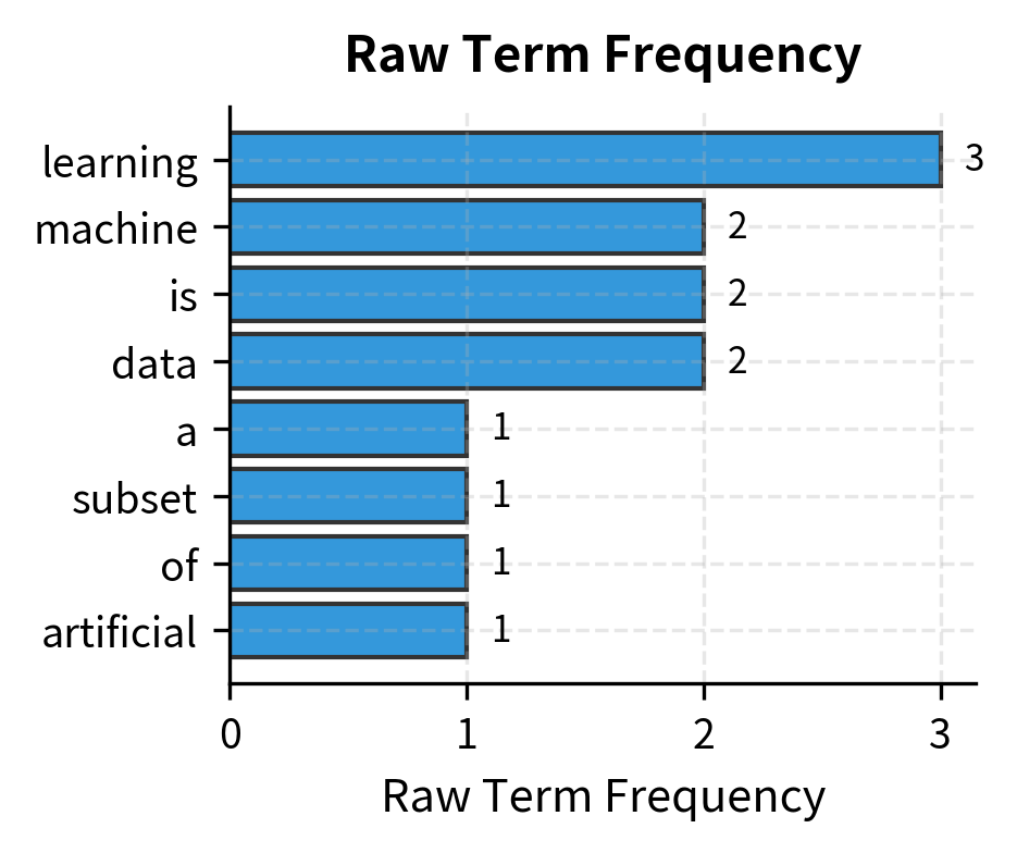
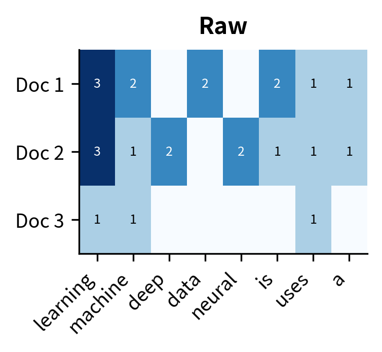
The output shows clear topical signatures for each document. "Learning" dominates Document 1 with 4 occurrences, making it the most characteristic term. Document 2 shows "deep" and "neural" as distinguishing features, reflecting its focus on deep learning. However, the results also reveal a problem: common words like "is" and "a" appear frequently across all documents without carrying meaningful semantic content. These function words inflate raw counts without adding discriminative power.
The Problem with Raw Counts
Raw term frequency has a proportionality problem. If "learning" appears twice as often as "data", does that mean it's twice as important? Probably not. The relationship between word count and importance is sublinear: the difference between 1 and 2 occurrences is more significant than the difference between 10 and 11.
The results expose the proportionality problem: "machine" appears 6 times, suggesting it's 6× more important than "science" (1 occurrence) and 3× more important than "data" (2 occurrences). But this linear relationship doesn't match intuition—a document mentioning "machine" six times isn't necessarily six times more about machines. After the first few occurrences, additional repetitions add diminishing information. This observation motivates log-scaled term frequency.
Term Frequency Distribution
Before moving to log-scaling, let's examine how term frequencies distribute across a document. Natural language follows Zipf's law: a few words appear very frequently, while most words appear rarely.

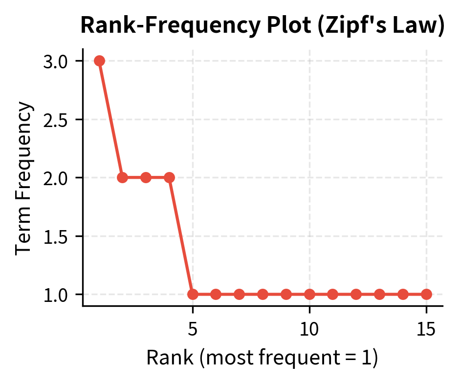
The rank-frequency plot shows the characteristic "long tail" of natural language: frequency drops rapidly with rank. Log-scaling addresses this by compressing the high-frequency end of this distribution.
Log-Scaled Term Frequency
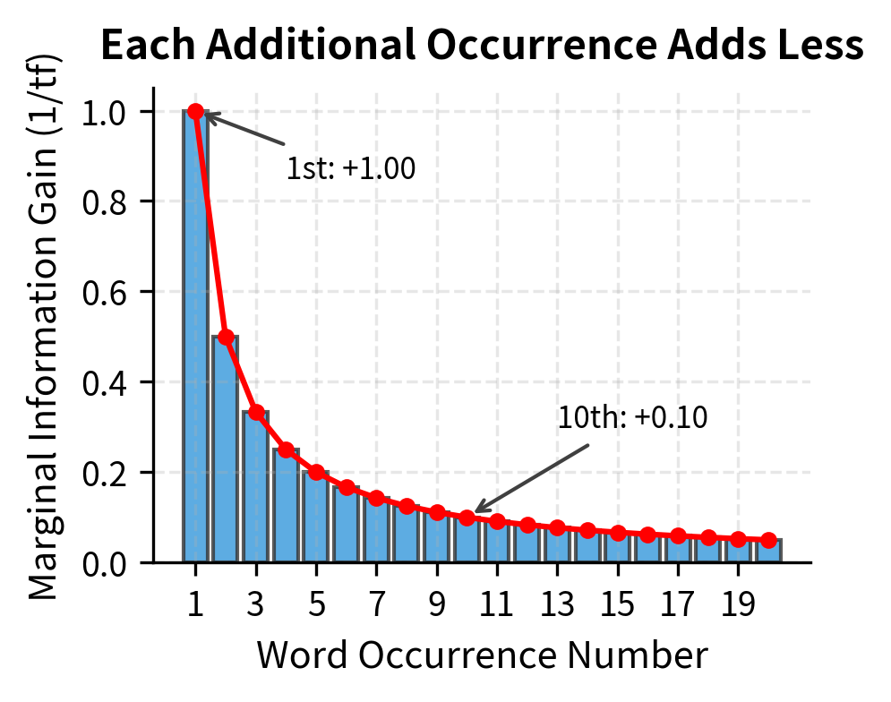
The proportionality problem reveals that raw counts make a flawed assumption: each additional word occurrence carries equal weight. But information doesn't work this way. The first time a document mentions "quantum," we learn something significant—this document touches on quantum topics. The second mention reinforces this. By the tenth mention, we're no longer learning much new; we already know the document focuses on quantum concepts.
This observation—that information gain diminishes with repetition—leads us to seek a mathematical function that captures this diminishing returns property. We need a transformation that:
- Preserves ordering: More occurrences should still mean higher weight (we don't want to lose ranking information)
- Compresses differences: The gap between 10 and 11 occurrences should be smaller than the gap between 1 and 2
- Grows sublinearly: The function should rise quickly at first, then flatten
The logarithm is precisely such a function. It's the mathematical embodiment of diminishing returns.
Why Logarithms?
The logarithm has a special property: it converts multiplicative relationships into additive ones. If one term appears 10 times more often than another, the log-scaled difference is just , not 10. This compression naturally models how information works—the first mention is highly informative, but repetition adds progressively less.
Mathematically, the derivative of is . This means the "rate of information gain" from each additional occurrence is inversely proportional to how many times we've already seen the word. The 10th occurrence adds only 1/10th as much as the first.
Log-scaled term frequency dampens the effect of high counts using the natural logarithm:
where:
- : the raw count of term in document
- : the natural logarithm (base )
- : the offset of ensures that a term appearing exactly once receives weight 1 (since , we get )
- The piecewise definition handles absent terms: if a word doesn't appear (), its weight is 0, not (which would produce)
Understanding the Formula
The formula is carefully constructed. The offset serves a critical purpose: since , a term appearing exactly once would otherwise get weight 0, making it indistinguishable from absent terms. Adding 1 ensures that a term appearing once gets weight 1.
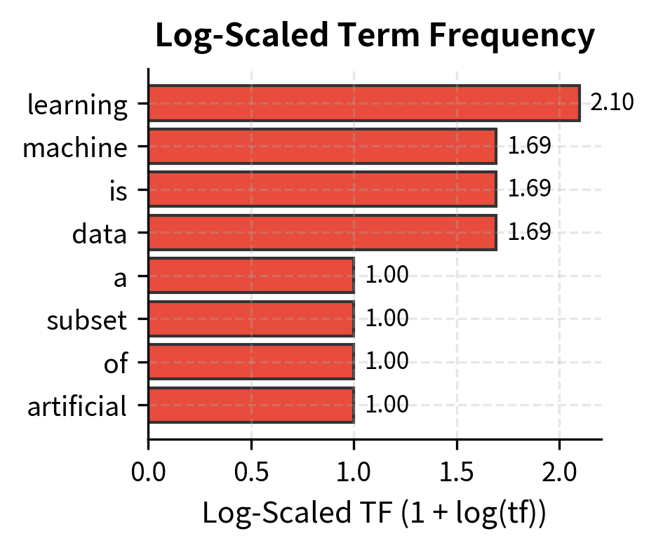
Let's trace through what happens at different frequency levels:
| Raw Count | Calculation | Log-Scaled Weight |
|---|---|---|
| 1 | 1.00 | |
| 2 | 1.69 | |
| 10 | 3.30 | |
| 100 | 5.61 |
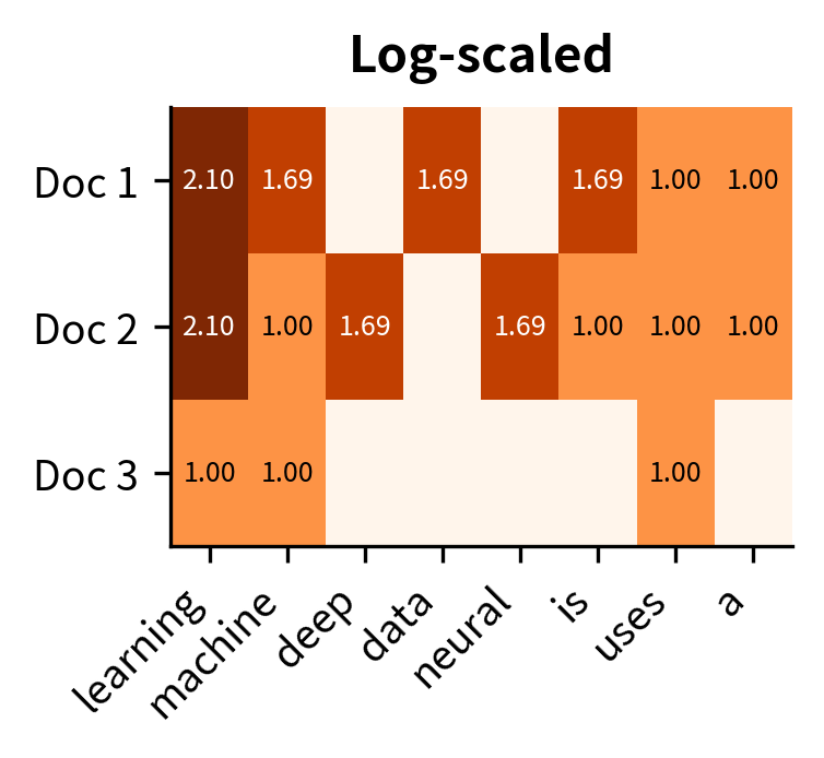
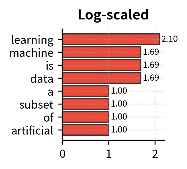
The 100x increase in raw count becomes only a 5.6x increase in log-scaled weight. A term appearing 100 times doesn't dominate one appearing once. It's weighted roughly 5-6 times higher, not 100 times.
The "Ratio" column reveals the compression effect. Terms with raw count 1 have ratio 1.0 (no change), but "learning" with 4 occurrences has a ratio of about 1.66—meaning log-scaling reduced its relative weight. The log TF of 2.39 for "learning" is only about 2.4× the weight of a single-occurrence term, not 4×. This compression better reflects how the fourth mention of a word adds less information than the first.
Visualizing the Log Transformation
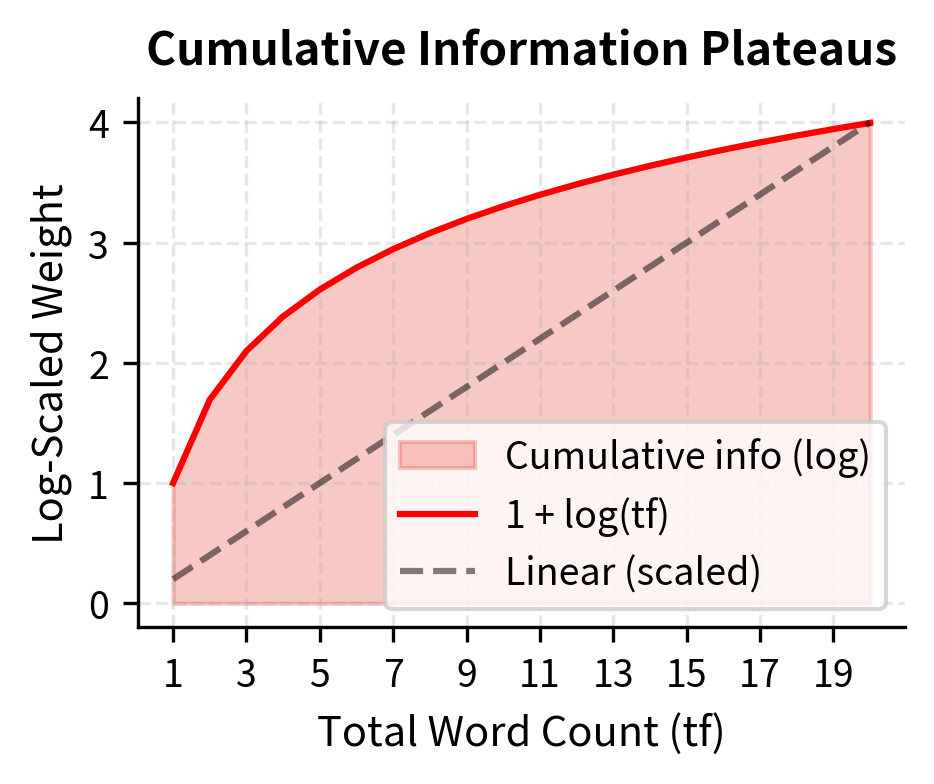
The logarithm's compression effect becomes clearer when we plot raw counts against their log-scaled equivalents:
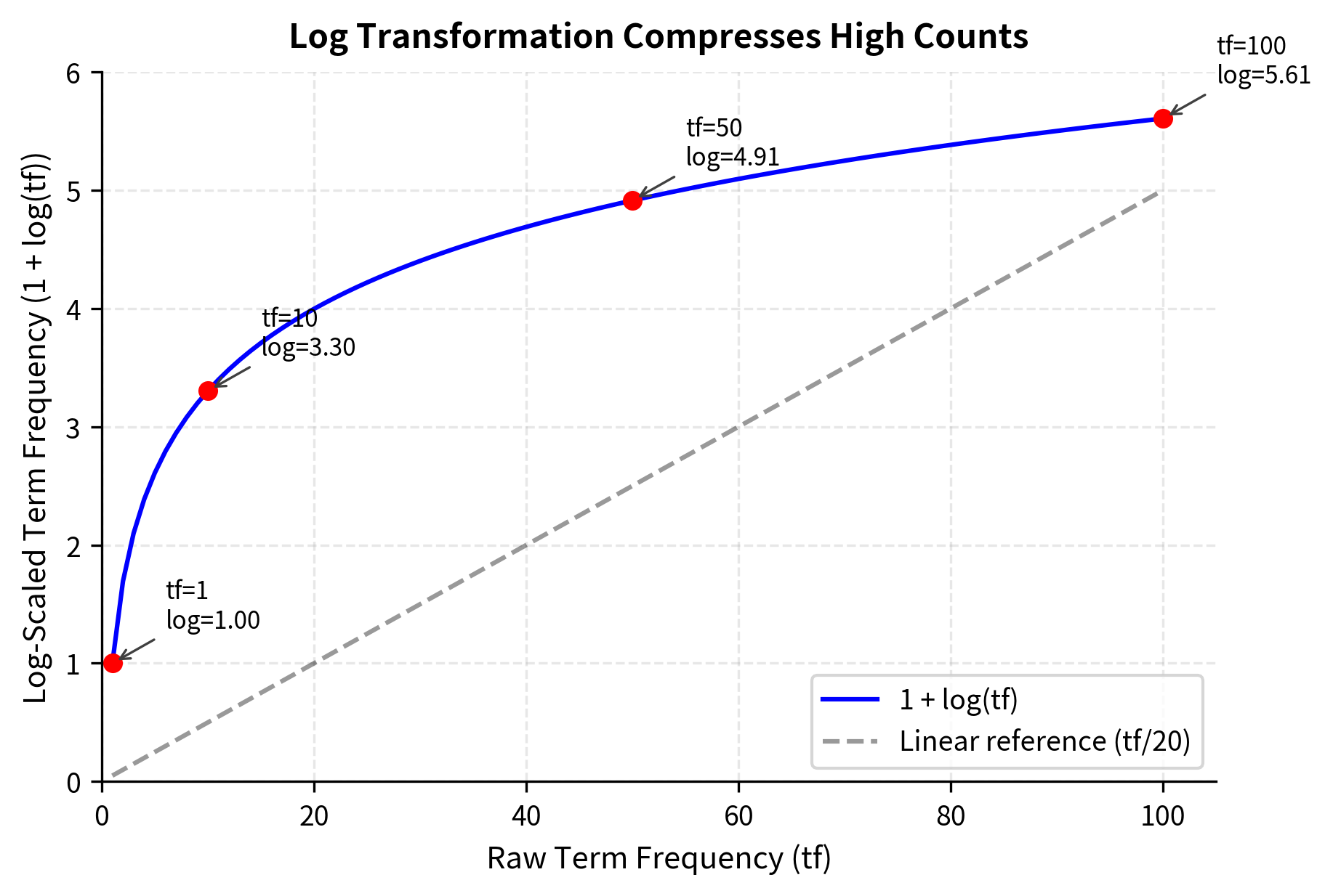
The curve flattens as raw counts increase. This sublinear relationship captures the intuition that the 10th occurrence of a word adds less information than the first.
Boolean Term Frequency
Log-scaling represents one response to the diminishing returns problem: compress high counts while preserving relative ordering. But what if we take this philosophy to its logical extreme? If the 100th occurrence of a word adds almost no information beyond the first, perhaps we should ignore counts entirely and focus on a simpler question: does this word appear at all?
This reasoning leads to boolean term frequency, the most aggressive form of count compression. It reduces the entire frequency distribution to a binary signal: present or absent, 1 or 0. A document mentioning "neural" once is indistinguishable from one mentioning it a hundred times.
At first glance, this seems to discard valuable information. But boolean TF embodies a specific philosophy about what matters: topic coverage rather than topic emphasis. When classifying documents into categories, knowing that a document discusses machine learning, neural networks, and optimization might matter more than knowing exactly how many times each term appears.
Boolean term frequency reduces frequency to a binary presence indicator:
where:
- : the term being queried—the word we're checking for
- : the document being analyzed
- : the set membership notation indicating that term appears at least once in document
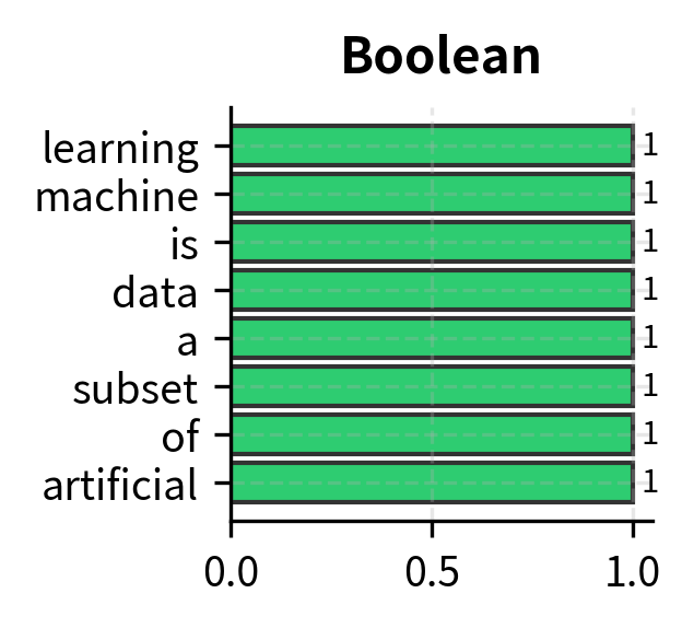
The output is binary: 1 if the word exists anywhere in the document, 0 if it's completely absent. All frequency information is collapsed into this single bit.
This might seem like throwing away information, but boolean TF excels when:
- You care about topic coverage, not emphasis
- Repeated terms might indicate spam or manipulation
- The task is set-based (does this document mention these concepts?)
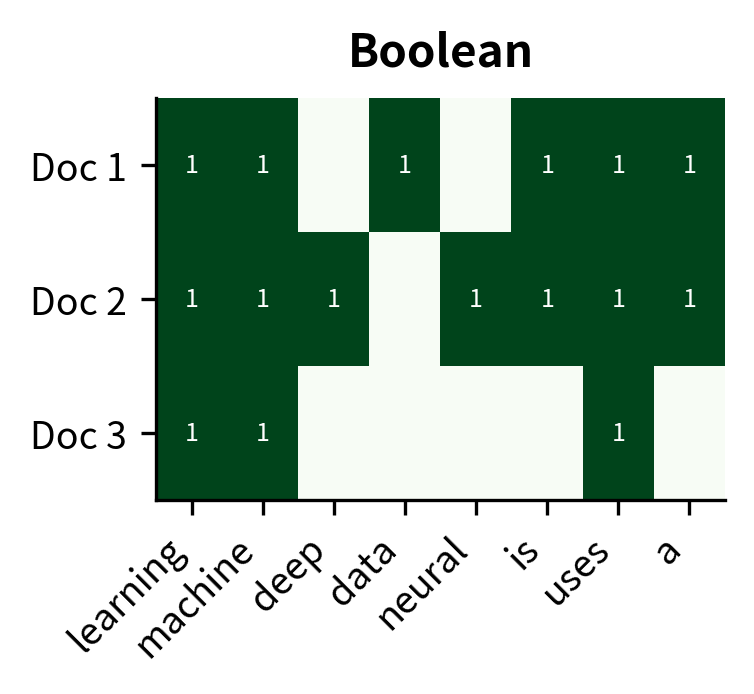
The comparison highlights the trade-offs between variants. "Learning" with 4 raw occurrences becomes 2.39 after log-scaling and just 1 with boolean TF. Similarly, "powerful" (1 occurrence) remains 1.00 across log and boolean but with very different implications: log-scaled 1.00 means "appeared once," while boolean 1 means "appeared at all." Boolean TF treats "learning" (4 occurrences) and "powerful" (1 occurrence) identically. This might seem like information loss, but for topic detection tasks, knowing a document mentions "learning" matters more than how often.
Augmented Term Frequency
So far, we've transformed individual term counts—compressing them with logarithms or collapsing them to binary indicators. But we've ignored a confounding factor that affects all these approaches: document length. A 10,000-word document will naturally contain more occurrences of any term than a 100-word document, even if both discuss the same topic with equal emphasis.
This length bias corrupts comparisons. When ranking documents by relevance to a query, we might inadvertently favor long documents simply because they have more words—not because they're more relevant. We need a normalization scheme that makes term frequencies comparable across documents of wildly different lengths.
The Document Length Problem
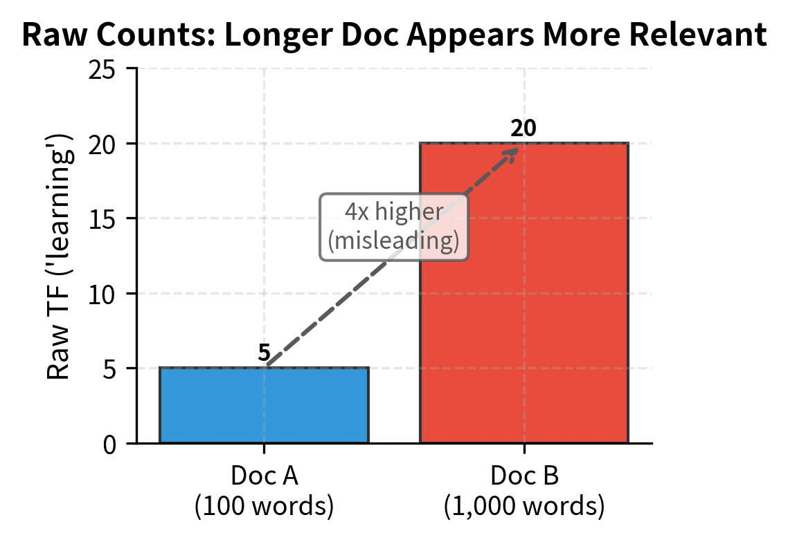
Consider a concrete example. Two documents about machine learning:
- Document A (100 words): mentions "learning" 5 times
- Document B (1,000 words): mentions "learning" 20 times
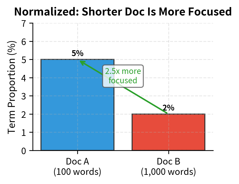
Which document is more focused on learning? Raw counts point to Document B (20 > 5). But this conclusion is misleading. Document A dedicates 5% of its words to "learning," while Document B dedicates only 2%. By the proportional measure, the shorter document is more focused on the topic, not less.
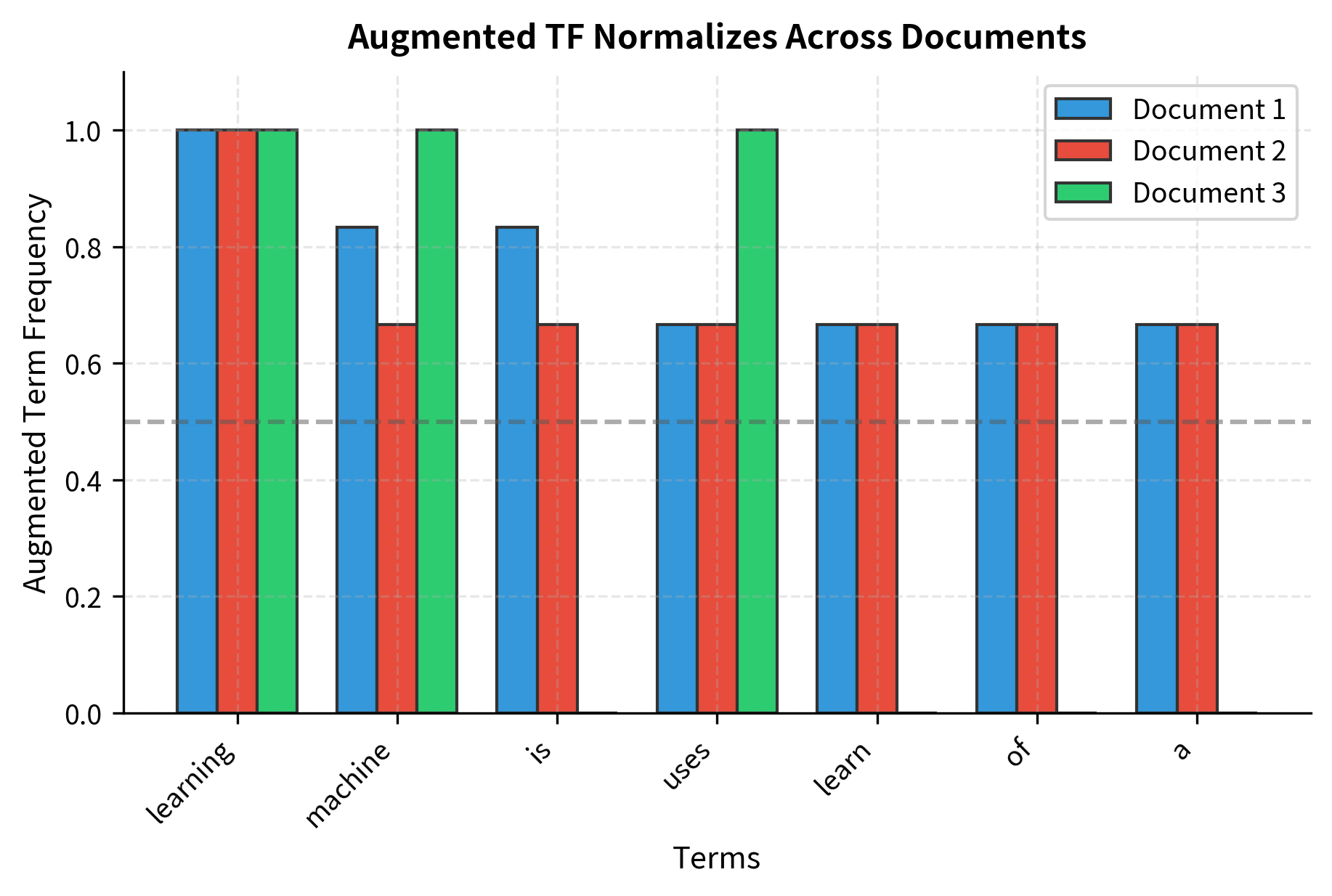
Augmented term frequency addresses this by reframing the question. Instead of asking "how many times does this term appear?", it asks: "how important is this term relative to the most important term in this document?"
The insight is that every document has a dominant term—the word that appears most frequently. By measuring other terms against this internal reference point, we create a scale that's consistent across documents regardless of their length. A term with half the count of the dominant term gets weight 0.75, whether that means 5 out of 10 occurrences or 500 out of 1,000.
Augmented term frequency (also called "double normalization" or "augmented normalized term frequency") normalizes each term against the document's maximum term frequency:
where:
- : the term being weighted—the specific word we're computing a weight for
- : the document being analyzed
- : the raw count of term in document
- : the highest term frequency in document —this notation means "find the maximum of over all terms that appear in "
- The ratio expresses each term's frequency as a fraction of the maximum, yielding values in
- The transformation maps this range to , ensuring all present terms receive at least baseline weight
Deconstructing the Formula
The formula has two components working together:
Step 1: Compute the relative frequency
First, we express each term's count as a fraction of the maximum count in the document:
where:
- : the raw count of term in document
- : the count of the most frequent term in document (this notation means "the maximum of over all terms that appear in ")
This ratio normalizes each term against the document's most frequent term, producing values between 0 and 1. The most frequent term gets 1.0; a term appearing half as often gets 0.5.
Step 2: Apply the double normalization
Next, we transform the relative frequency to provide a baseline weight for all terms:
The constants 0.5 and 0.5 are design choices that produce the "double normalization" scheme (also called "augmented normalized term frequency"). This transformation maps the [0, 1] range to [0.5, 1.0]. Why not just use the ratio directly? The 0.5 baseline ensures that even rare terms receive meaningful weight, preventing them from being completely overshadowed by the dominant term.
The formula guarantees:
- The most frequent term in any document gets weight 1.0
- All other terms get weights between 0.5 and 1.0, proportional to their relative frequency
- All documents are on a comparable scale regardless of length
![The augmented TF transformation maps relative frequencies [0,1] to [0.5,1.0]. The 0.5 baseline ensures rare terms maintain meaningful weight.](https://cnassets.uk/notebooks/6_term_frequency_files/augmented-tf-transformation-curve.png)
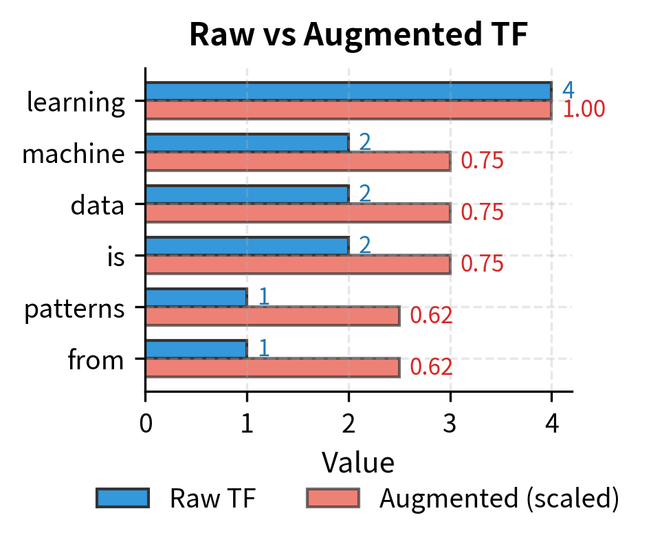
Each document's most frequent term receives weight 1.0 (the maximum), while other terms scale proportionally into the [0.5, 1.0] range. Notice how Document 1's "learning" (raw=4) gets 1.000, while "machine" (raw=2) gets 0.750—exactly . The baseline of 0.5 ensures that even terms appearing once receive meaningful weight (0.625 when max_tf=4). This normalization makes cross-document comparison fairer by eliminating the advantage longer documents would otherwise have.
L2-Normalized Frequency Vectors
Augmented TF normalizes against a single reference point—the document's most frequent term. But this approach ignores the broader context of how all terms relate to each other. What if we want a normalization that considers the entire term frequency distribution at once?
This question leads us to think geometrically. Each document's term frequencies can be viewed as coordinates in a high-dimensional space, where every vocabulary word defines an axis. A document with frequencies [4, 0, 2, 1, ...] becomes a point (or equivalently, a vector from the origin to that point) in this space. This geometric perspective reveals a crucial insight: the vector has two distinct properties:
- Direction: which terms the document emphasizes (its topical content)
- Magnitude: how many total word occurrences it contains (related to length)
For comparing document content, only direction matters. Magnitude confounds the comparison by favoring longer documents.
From Counts to Geometry
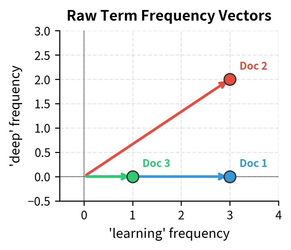
To build intuition, imagine a vocabulary of just two words: "learning" and "deep". Each document becomes a point in 2D space:
- Document with TF = [4, 0] points along the "learning" axis—purely about learning
- Document with TF = [2, 2] points diagonally at 45°—equal emphasis on both topics
- Document with TF = [0, 3] points along the "deep" axis—purely about deep learning
The angle between two document vectors captures their semantic similarity. Documents pointing in similar directions discuss similar topics; documents at right angles share nothing in common. The length of each vector, however, merely reflects word count—a confounding factor we want to eliminate.
L2 normalization achieves exactly this: it projects every document onto the unit sphere, preserving direction while forcing all vectors to have the same magnitude (length 1). Two documents with identical word proportions but different lengths will map to the same point on the unit sphere.
L2 normalization divides each term frequency by the vector's Euclidean length, projecting the document onto the unit sphere:
where:
- : the raw count of term in document —the numerator
- : notation meaning "for all terms that appear in document "
- : the squared frequency of each term
- : the sum of all squared term frequencies in the document
- : the L2 norm (Euclidean length) of the TF vector, often written compactly as
Why squared counts? The L2 norm generalizes the Pythagorean theorem to dimensions. In 2D, a vector has length . In dimensions, we sum all squared components and take the square root. Dividing every component by this length scales the vector to unit length () while preserving its direction.
Practical benefit: After L2 normalization, cosine similarity between two documents becomes a simple dot product—no need to compute norms during comparison.
Why the L2 Norm?
The L2 norm (also called the Euclidean norm) measures the straight-line distance from the origin to the tip of the vector. For a vector , the L2 norm is computed as:
This formula generalizes the Pythagorean theorem to dimensions. Dividing each element of the vector by this norm scales the vector to length 1 while preserving its direction. After normalization, every document vector lies on the surface of a unit hypersphere.
This geometric property has a practical benefit: the angle between any two normalized vectors directly measures their content similarity. Documents pointing in similar directions (small angle) have high cosine similarity; documents pointing in different directions (large angle) are dissimilar.
L2 normalization is particularly useful for:
- Efficient similarity computation: Cosine similarity becomes a simple dot product
- Length-invariant comparison: A 100-word and 10,000-word document on the same topic will have similar normalized vectors
- ML compatibility: Many machine learning models assume or benefit from normalized inputs
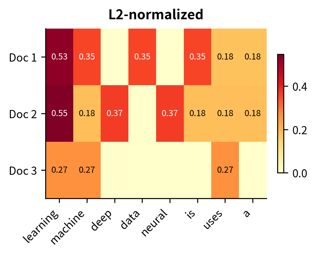
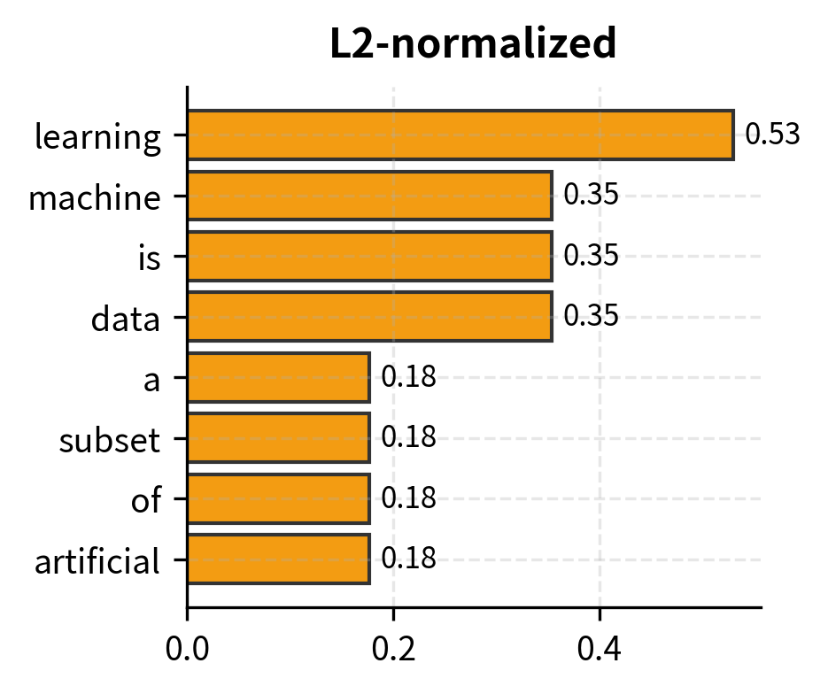
The vector norm of 1.0000 for each document confirms successful L2 normalization—all documents now lie on the unit hypersphere. The individual term weights are smaller than other TF variants because they must sum (in squares) to 1. For Document 1, "learning" contributes about 0.53 to the unit vector's direction, making it the dominant component. These normalized values enable efficient similarity computation: the dot product of any two L2-normalized vectors directly gives their cosine similarity.
Geometric Interpretation: Vectors on the Unit Sphere
L2 normalization projects all document vectors onto the surface of a unit hypersphere. In high dimensions this is hard to visualize, but we can illustrate the concept by projecting our documents into 2D using their two most distinctive terms:
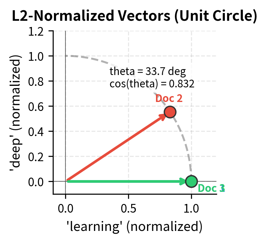
On the unit circle, the angle θ between vectors directly measures semantic distance. Documents pointing in similar directions (small θ) have high cosine similarity; documents pointing in different directions (large θ) are dissimilar.
Cosine Similarity with Normalized Vectors
The practical benefit of L2 normalization becomes clear when computing document similarity. Cosine similarity measures the angle between two vectors. Given two document vectors and , cosine similarity is defined as:
where:
- : term frequency vectors for two documents, where each element or represents the frequency of term
- : the dot product, which sums the element-wise products across all vocabulary terms
- : the L2 norm (Euclidean length) of vector
The numerator captures how much the vectors "agree" (shared terms with high counts contribute positively), while the denominator normalizes by the vectors' magnitudes to ensure the result falls between -1 and 1 (or 0 and 1 for non-negative term frequencies).
When both vectors are already L2-normalized (), the denominator becomes 1, and cosine similarity reduces to a simple dot product:
This simplification speeds up computation: comparing millions of documents becomes a matrix multiplication rather than millions of individual normalizations.
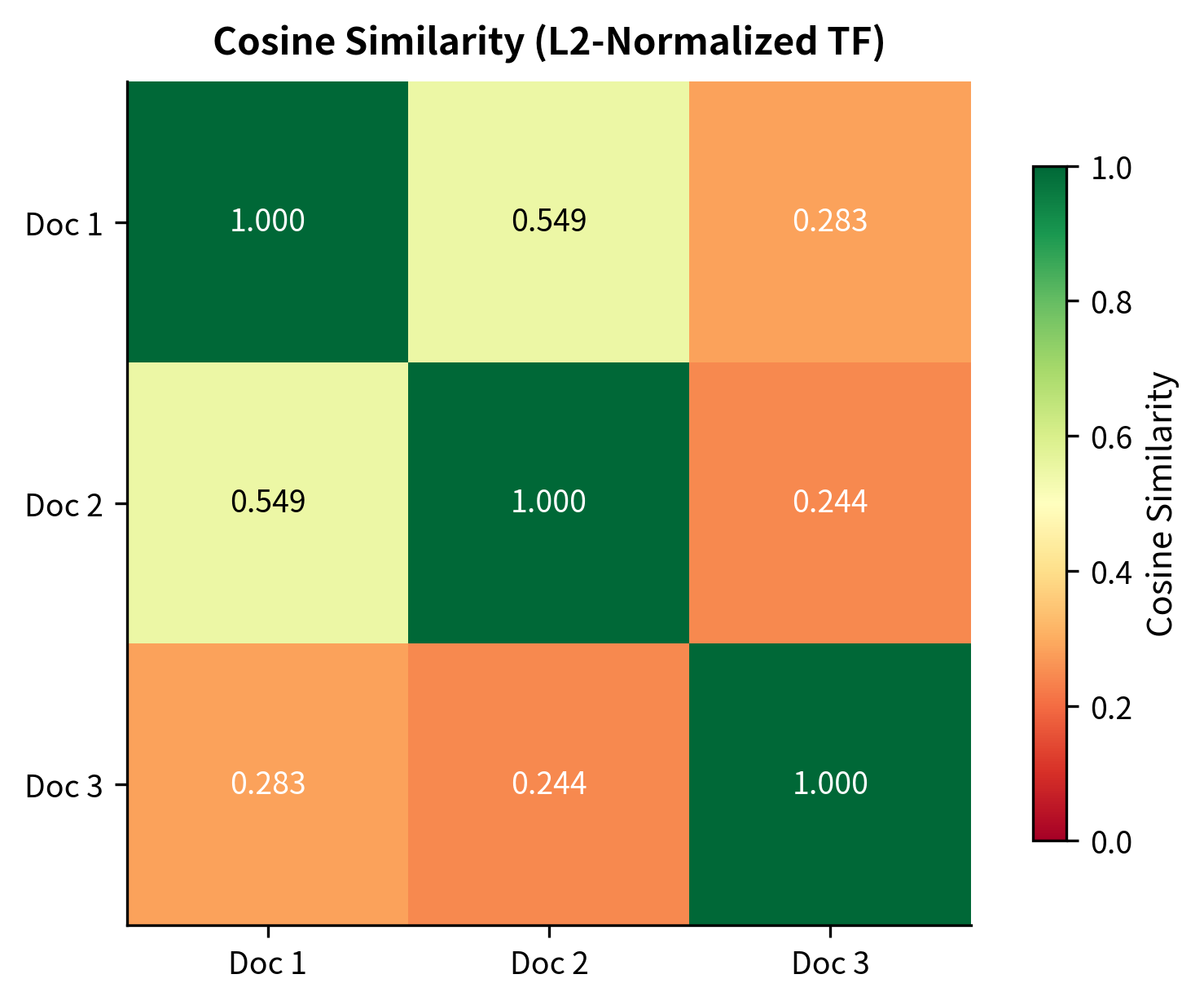
The diagonal values of 1.000 confirm that each document is perfectly similar to itself (as expected). The off-diagonal values reveal document relationships: Documents 1 and 2 show the highest similarity (both discuss machine learning and deep learning concepts with shared vocabulary like "learning" and "machine"). Document 3, focused on NLP, shows lower similarity to both—it shares some terms like "machine" and "learning" but introduces distinct vocabulary like "text", "classification", and "sentiment".
Term Frequency Sparsity Patterns
We've explored five ways to weight term frequencies, each with different mathematical properties. But before choosing among them, we need to understand a practical reality that affects all term frequency representations: sparsity.
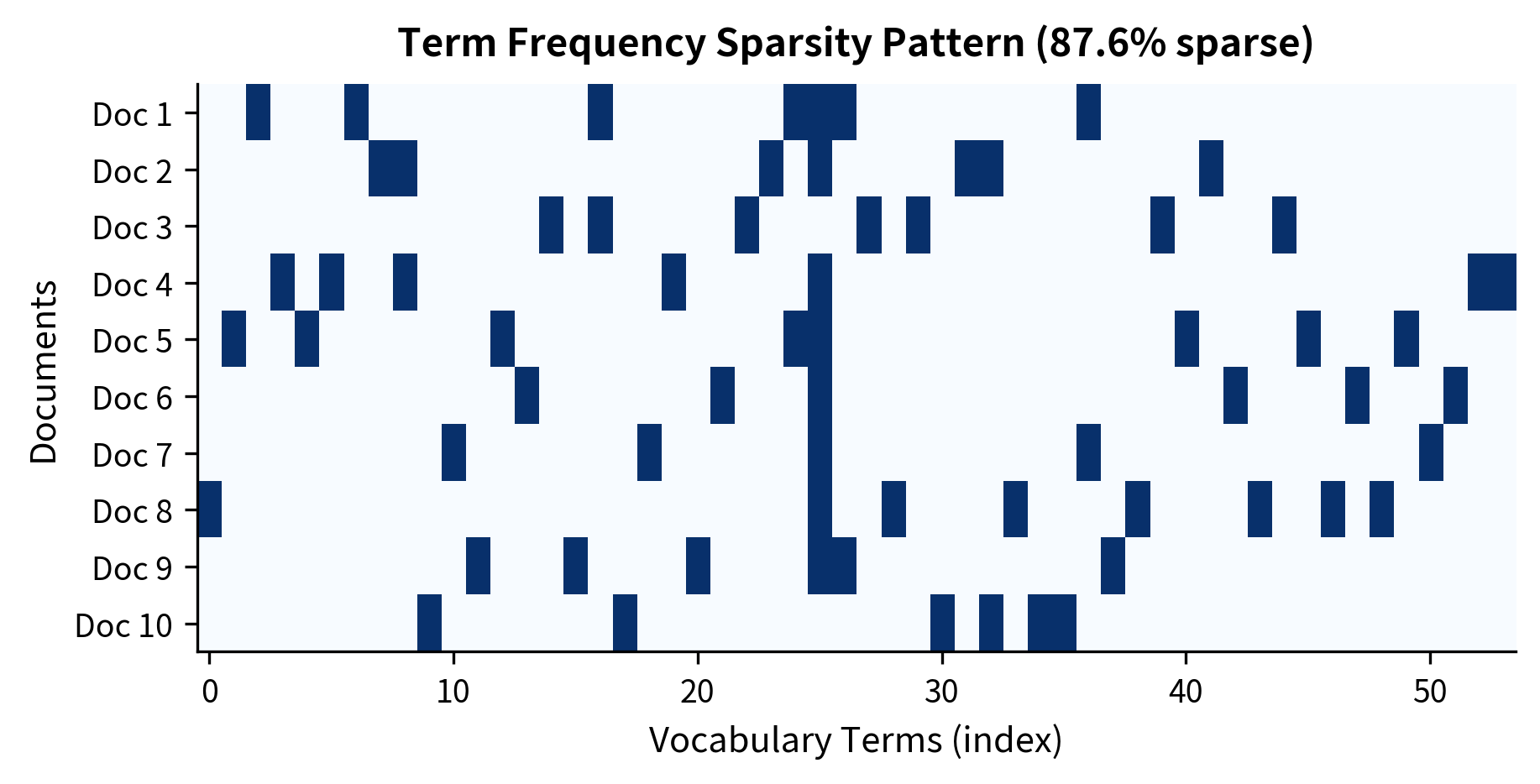
Real-world term frequency matrices are extremely sparse. A typical English vocabulary contains tens of thousands of words, yet any individual document uses only a few hundred. This means most entries in a document-term matrix are zero. Understanding this sparsity matters for efficient computation and storage.
Even this tiny corpus demonstrates high sparsity. With only 6-7 unique terms per document out of 50+ vocabulary words, over 84% of matrix entries are zero. The "average documents per term" metric of ~1.6 indicates most words appear in only one or two documents—a characteristic of natural language where specialized terms have narrow usage.
In production systems with vocabularies of 100,000+ words and documents averaging 200 unique terms, sparsity typically exceeds 99.9%. This extreme sparsity makes dense matrix storage impractical (imagine storing 100 billion zeros for a million-document corpus) and sparse formats essential.
Sparsity Implications
High sparsity has practical consequences:
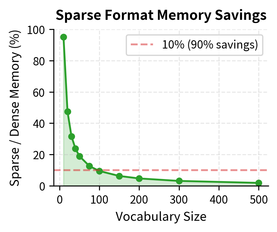
Memory efficiency: Sparse matrix formats (CSR, CSC) store only non-zero values, reducing memory by orders of magnitude.
Computation speed: Sparse matrix operations skip zero elements, dramatically speeding up matrix multiplication and similarity calculations.
Feature selection: Many terms appear in very few documents, contributing little discriminative power. Pruning rare terms reduces dimensionality without losing much information.
The sparse CSR format achieves substantial memory savings even on this small matrix. The compression ratio directly reflects sparsity: at 84% sparsity, we save roughly 60% of memory. At production-scale sparsity (99%+), the ratio improves dramatically—a corpus of 1 million documents with 100,000 vocabulary terms could shrink from 800 GB (dense float64) to under 10 GB with sparse storage. This difference often determines whether an application fits in memory at all.
How Sparsity Scales with Vocabulary Size
As vocabulary grows, sparsity increases dramatically. This plot shows the relationship between vocabulary size and matrix sparsity:
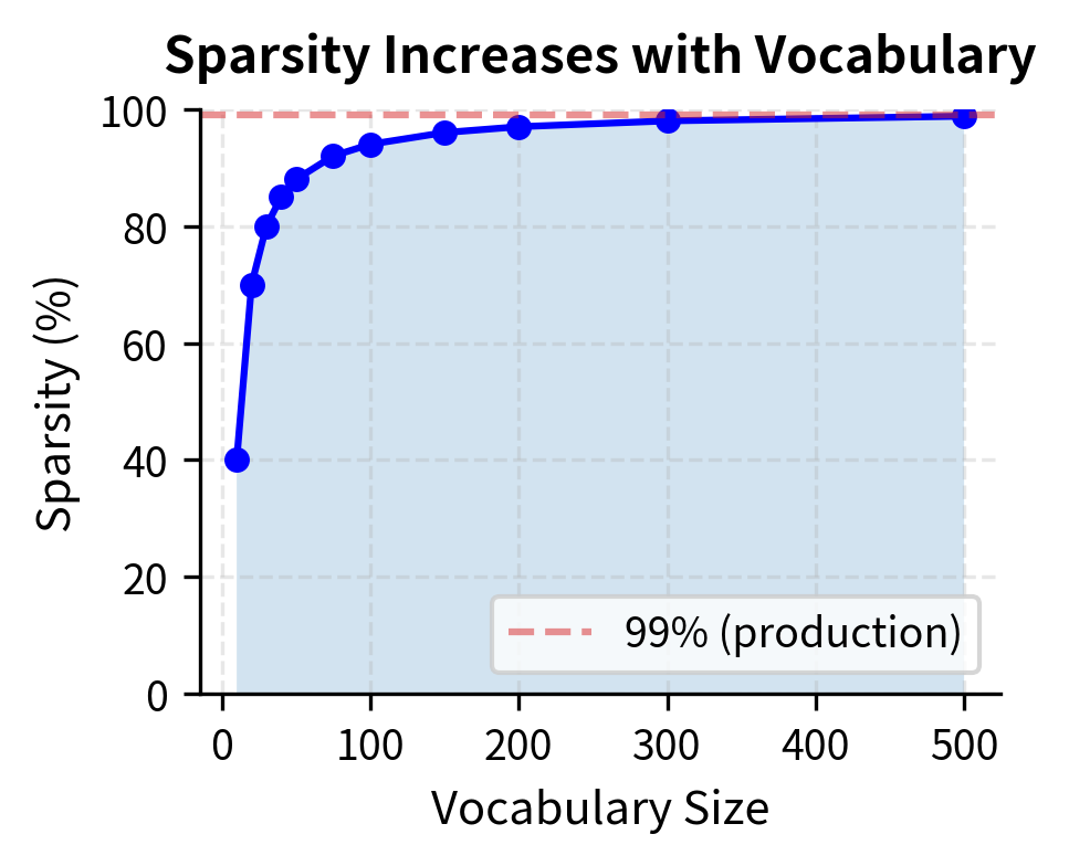
The key insight: document length stays roughly constant as vocabulary grows, so the ratio of non-zero to total entries shrinks. This is why sparse matrix formats become essential at scale.
Efficient Term Frequency Computation
For production systems, efficiency matters. Let's compare different approaches to computing term frequency:
The benchmark demonstrates scikit-learn's significant performance advantage. The speedup comes from multiple optimizations: compiled Cython/C code paths, efficient sparse matrix construction that avoids intermediate dense allocations, and vectorized string operations. The manual Counter approach requires Python-level iteration and dictionary operations, which carry interpreter overhead.
For production applications processing thousands or millions of documents, this performance gap becomes critical. Always prefer library implementations over custom code unless you have specific requirements they can't meet.
CountVectorizer TF Variants
CountVectorizer supports different term frequency schemes through its parameters:
The output demonstrates scikit-learn's flexibility in producing different TF representations from the same input. Raw counts preserve exact frequencies (useful for models that can learn their own weighting), binary collapses all counts to 1 (ideal for set-based operations), and L2-normalized values create unit vectors ready for cosine similarity. Note that "learning" with raw count 4 becomes 0.5345 after L2 normalization—this reflects its proportional contribution to the document vector's direction. The L2 values will sum (in squares) to 1.0 across all terms in the document.
Choosing a TF Variant
We've now covered the full spectrum of term frequency weighting schemes, from raw counts to sophisticated normalizations. Each addresses a specific problem:
- Raw TF gives you the basic signal but overweights repetition
- Log-scaled TF compresses high counts, modeling diminishing returns
- Boolean TF ignores frequency entirely, focusing on presence
- Augmented TF normalizes within each document, handling length variation
- L2-normalized TF projects documents onto a unit sphere, enabling efficient similarity computation
Which variant should you use? It depends on your task:
| Variant | Formula | Best For |
|---|---|---|
| Raw | When exact counts matter, baseline models | |
| Log-scaled | General purpose, TF-IDF computation | |
| Boolean | if present, else | Topic detection, set-based matching |
| Augmented | Cross-document comparison, length normalization | |
| L2-normalized | Cosine similarity, neural network inputs |
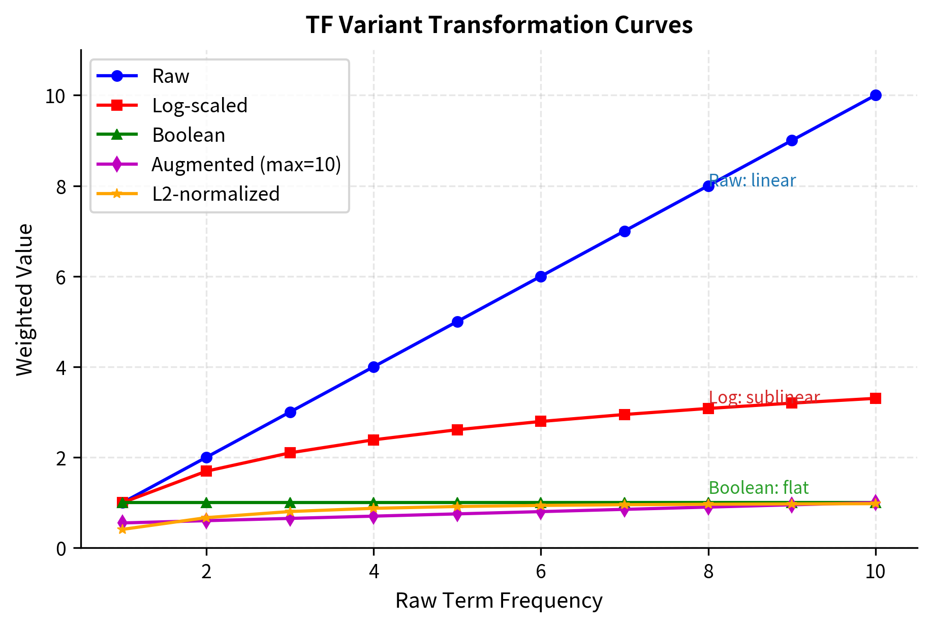
The transformation curves reveal each variant's philosophy: raw TF treats all counts linearly, log-scaled compresses high values, boolean ignores magnitude entirely, and augmented/L2 normalize relative to other terms.
![Augmented TF normalizes by maximum term frequency, producing values in [0.5, 1.0].](https://cnassets.uk/notebooks/6_term_frequency_files/tf-variants-heatmap-augmented.png)

![Augmented TF normalizes by max frequency. All values fall in [0.5, 1.0].](https://cnassets.uk/notebooks/6_term_frequency_files/tf-variants-comparison-augmented.png)
Limitations and Impact
Term frequency, in all its variants, captures only one dimension of word importance: how often a term appears in a document. This ignores a key question: how informative is this term across the entire corpus?
The "the" problem: Common words like "the", "is", and "a" appear frequently in almost every document. High TF doesn't distinguish documents when every document has high TF for the same words.
No corpus context: TF treats each document in isolation. A term appearing 5 times might be significant in a corpus where it's rare, or meaningless in a corpus where every document mentions it.
Length sensitivity: Despite normalization schemes, longer documents naturally contain more term occurrences, potentially biasing similarity calculations.
These limitations motivate Inverse Document Frequency (IDF), which we'll cover in the next chapter. IDF asks: how rare is this term across the corpus? Combining TF with IDF produces TF-IDF, one of the most successful text representations in information retrieval.
Term frequency laid the groundwork for quantifying word importance. The variants we explored, raw counts, log-scaling, boolean, augmented, and L2-normalized, each address different aspects of the counting problem. Understanding these foundations prepares you to appreciate why TF-IDF works and when to use its variants.
Summary
Term frequency transforms word counts into weighted signals of importance. The key variants each serve different purposes:
- Raw term frequency counts occurrences directly, but overweights repeated terms
- Log-scaled TF () compresses high counts, capturing diminishing returns of repetition
- Boolean TF reduces to presence/absence, useful when topic coverage matters more than emphasis
- Augmented TF normalizes by maximum frequency, enabling fair cross-document comparison
- L2-normalized TF creates unit vectors, making cosine similarity a simple dot product
Term frequency matrices are extremely sparse in practice, with 99%+ zeros for realistic vocabularies. Sparse matrix formats and optimized libraries like scikit-learn's CountVectorizer make efficient computation possible.
The main limitation of TF is its document-centric view. A term appearing frequently might be common across all documents (uninformative) or rare and distinctive. The next chapter introduces Inverse Document Frequency to address this, setting the stage for TF-IDF.
Key Functions and Parameters
When working with term frequency in scikit-learn, two classes handle most use cases:
CountVectorizer(lowercase, min_df, max_df, binary, ngram_range, max_features)
lowercase(default:True): Convert text to lowercase before tokenization. Disable for case-sensitive applications.min_df: Minimum document frequency. Integer for absolute count, float for proportion. Usemin_df=2to remove typos and rare words.max_df: Maximum document frequency. Usemax_df=0.95to filter extremely common words.binary(default:False): Set toTruefor boolean term frequency where only presence matters.ngram_range(default:(1, 1)): Tuple of (min_n, max_n). Use(1, 2)to include bigrams.max_features: Limit vocabulary to top N most frequent terms for dimensionality control.
TfidfVectorizer(use_idf, norm, sublinear_tf)
use_idf(default:True): Set toFalseto compute only term frequency without IDF weighting.norm(default:'l2'): Vector normalization. Use'l2'for cosine similarity,'l1'for Manhattan distance, orNonefor raw values.sublinear_tf(default:False): Set toTrueto apply log-scaling: replaces tf with .
Quiz
Ready to test your understanding? Take this quick quiz to reinforce what you've learned about term frequency weighting schemes.

Comments