

Master beam search decoding for sequence-to-sequence models. Learn log probability scoring, length normalization, diverse beam search, and when to use sampling.

This article is part of the free-to-read Language AI Handbook
Choose your expertise level to adjust how many terms are explained. Beginners see more tooltips, experts see fewer to maintain reading flow. Hover over underlined terms for instant definitions.
Beam Search
When a sequence-to-sequence model generates output, it faces a fundamental challenge: at each timestep, it must choose from thousands of possible tokens. The simplest approach, greedy decoding, picks the single most probable token at each step. But this myopic strategy often leads to suboptimal sequences because a locally good choice can paint the model into a corner, forcing poor choices later. Beam search offers a principled middle ground between exhaustive search (computationally impossible) and greedy decoding (often suboptimal), maintaining multiple candidate sequences simultaneously to find better overall translations.
The Problem with Greedy Decoding
Greedy decoding selects the highest-probability token at each timestep, building the output sequence one token at a time. While computationally efficient, this approach has a critical flaw: it cannot recover from early mistakes.
Consider translating "The cat sat on the mat" into French. At the first timestep, suppose the model assigns these probabilities:
- "Le" (The, masculine): 0.45
- "La" (The, feminine): 0.35
- "Un" (A, masculine): 0.15
- "Une" (A, feminine): 0.05
Greedy decoding picks "Le" with probability 0.45. But what if "La chatte" (the female cat) would lead to a more fluent overall translation? The greedy decoder cannot explore this path once it commits to "Le."
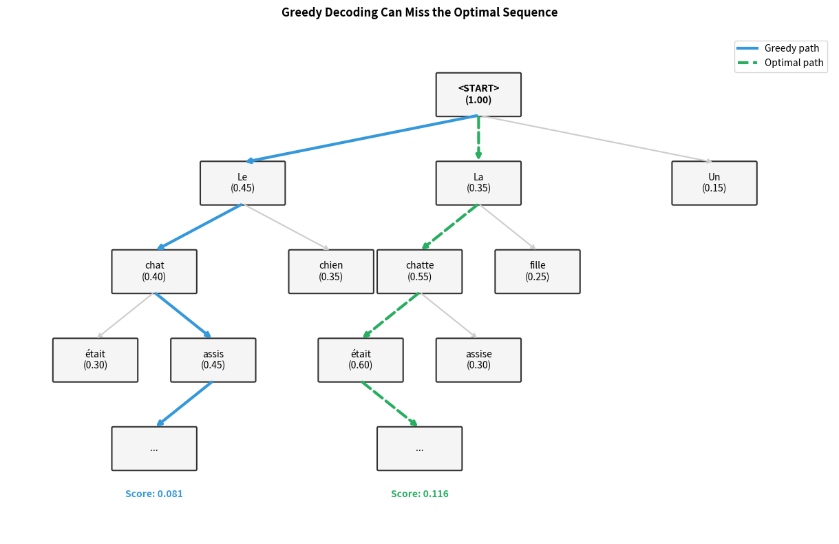
The greedy path achieves a cumulative probability of , while the alternative path through "La chatte était" achieves . Despite starting with a lower-probability token, the second path is 43% more likely overall. Greedy decoding cannot discover this because it never explores paths that start with suboptimal first choices.
This limitation becomes more severe as sequences grow longer. Each greedy decision constrains future options, and small early mistakes compound into significantly worse final translations. The model might generate grammatically correct but awkward or semantically imprecise text simply because it committed too early to a particular phrasing.
The Beam Search Algorithm
Having seen how greedy decoding can miss globally optimal sequences, we need an algorithm that explores multiple possibilities without the exponential cost of exhaustive search. Beam search provides exactly this: a principled way to maintain several candidate sequences simultaneously, hedging our bets until we have enough evidence to commit.
The Core Idea: Hedging Your Bets
Imagine you're navigating a maze where each intersection offers several paths forward. Greedy decoding is like always taking the path that looks most promising at each intersection. This is efficient, but you might walk into a dead end. Exhaustive search explores every possible route, guaranteed to find the best path, but impossibly slow for large mazes. Beam search takes a middle approach: at each intersection, you send scouts down the most promising paths, where is called the beam width.
The beam width controls how many candidate sequences beam search maintains at each step. A beam width of 1 reduces to greedy decoding. Typical values range from 4 to 10 for most applications, balancing exploration against computational cost.
Why does this work? Because natural language has structure. If "Le chat" (the male cat) leads to awkward phrasing, we want to discover this before committing. Keeping "La chatte" (the female cat) alive as an alternative lets us recover. The beam width determines how many "insurance policies" we maintain against early mistakes.
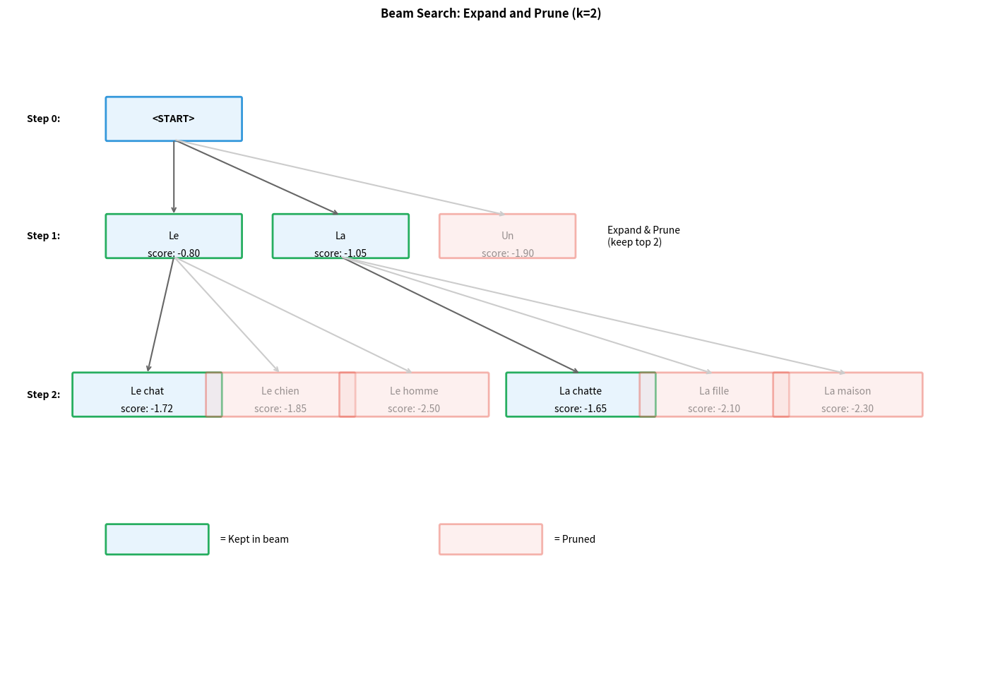
The Algorithm: Expand, Score, Prune, Repeat
Beam search follows a simple four-phase cycle at each timestep:
-
Expand: For each hypothesis currently in the beam, consider all possible next tokens. If we have hypotheses and a vocabulary of tokens, this generates candidate extensions.
-
Score: Assign each candidate a score reflecting how probable the entire sequence is so far. Higher scores indicate more promising sequences.
-
Prune: Keep only the top candidates by score. This is the key step that prevents exponential growth, ruthlessly discarding all but the best options.
-
Terminate: If a candidate ends with the
<END>token, move it to a "completed" list. Continue until all hypotheses are complete or we reach a maximum length.
The algorithm begins with a single hypothesis containing only <START> (score 0 in log space), and ends by returning the highest-scoring completed sequence.
The Scoring Function: Why Log Probabilities?
To compare hypotheses during beam search, we need a principled way to quantify "how good" a partial sequence is. This section develops the scoring function from first principles, showing why the mathematical choices we make are not arbitrary but rather necessary solutions to fundamental problems.
The Goal: Measuring Sequence Quality
When beam search maintains multiple candidate sequences, it must decide which ones to keep and which to discard. The natural measure of sequence quality is probability: given an input , how likely is the model to generate this particular output sequence?
For a sequence , we want to compute , the probability of generating exactly these tokens in this order, conditioned on the input. But how do we compute this joint probability when our model only predicts one token at a time?
From Single Tokens to Full Sequences: The Chain Rule
A sequence-to-sequence model generates output autoregressively: at each step, it predicts the next token based on the input and all previously generated tokens. This means we can decompose the joint probability using the chain rule:
Each factor is exactly what our model computes at timestep : the probability distribution over the next token, given the input and all tokens generated so far. The sequence probability is simply the product of all these per-token probabilities.
This decomposition is powerful because it lets us compute sequence probabilities incrementally. When we extend a hypothesis by one token, the new sequence probability is just the old probability multiplied by the new token's probability.
The Numerical Underflow Problem
While the chain rule gives us a mathematically correct formula, it creates a serious computational problem. Consider what happens as sequences grow longer.
Suppose each token has an average probability of 0.3 (a reasonable estimate for natural language). For a 20-token sequence:
This number is extraordinarily small, so small that standard 32-bit floating-point arithmetic may round it to exactly zero. Real sequences are often 50-100 tokens long, with many tokens having probabilities well below 0.3. Multiplying dozens of small numbers together quickly produces values that computers cannot represent.
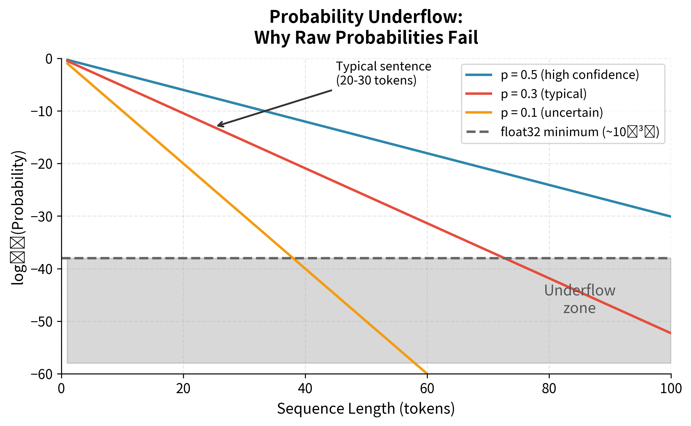
This isn't a theoretical concern. It's a practical bug that causes beam search to fail silently. When all sequence probabilities underflow to zero, the algorithm cannot distinguish between good and bad hypotheses.
The Solution: Working in Log Space
The solution is elegant: instead of tracking probabilities directly, we track their logarithms. This simple transformation solves the underflow problem while preserving everything we need for comparison.
Recall that for any positive numbers and :
This means that multiplying probabilities in regular space is equivalent to adding log probabilities in log space. Our problematic product becomes a well-behaved sum:
The benefits of this transformation are substantial:
-
Numerical stability: Log probabilities are moderate negative numbers. For , we have . Adding 20 such numbers gives , a perfectly manageable value that any computer can represent exactly.
-
Computational efficiency: Addition is faster than multiplication on most hardware, and the difference compounds over millions of sequence evaluations during decoding.
-
Preserved ordering: Since is a monotonically increasing function, if , then . Maximizing log probability is equivalent to maximizing probability, so we lose nothing by working in log space.
The Beam Search Scoring Formula
We can now state the scoring formula precisely. Given a partial output sequence generated from input , the score is the cumulative log probability:
where:
- : the output sequence from position 1 to , representing all tokens generated so far
- : the token at position in the output sequence
- : the prefix of all previously generated tokens (before position ); for , this is empty
- : the input sequence being translated or transformed
- : the model's predicted probability of token , conditioned on the input and all previous outputs
- : the natural logarithm, mapping probabilities from to
This formula has an elegant incremental property: when we extend a hypothesis by adding token , the new score is simply:
We don't need to recompute the entire sum; we just add one term. This makes beam search efficient even for long sequences.
Interpreting Scores
Understanding how to read scores is essential for debugging and intuition. Since probabilities lie in , their logarithms are non-positive:
- Scores are always ≤ 0: A score of 0 means probability 1 (impossible for real sequences). Typical scores range from to depending on sequence length.
- Higher (less negative) scores are better: A score of beats a score of .
- Scores are additive costs: Each token "costs" some negative amount. Better token choices cost less (smaller negative numbers).
To convert a score back to probability, exponentiate: . For example:
| Score | Probability | Interpretation |
|---|---|---|
| 10%, quite likely | ||
| 1%, plausible | ||
| 0.01%, unlikely |
The ratio of probabilities corresponds to the difference in scores. If hypothesis A has score and hypothesis B has score , then A is times more likely than B.
Implementing Beam Search
With the scoring function established, we can now implement beam search. Building the algorithm from scratch will solidify your understanding of how the expand-score-prune cycle operates and how log probabilities flow through the computation.
Step 1: Representing Hypotheses
A hypothesis is a candidate sequence under consideration. During beam search, we maintain multiple hypotheses simultaneously, each representing a different path through the token space. Every hypothesis must track two pieces of information:
- The tokens generated so far: The actual sequence of token IDs
- The cumulative score: The sum of log probabilities accumulated along this path
We represent this as a simple dataclass:
The extend method implements the incremental scoring property we derived earlier. When we add a new token with log probability log_prob, we create a new hypothesis with:
- The original tokens plus the new token appended
- The original score plus the new log probability (implementing )
This immutable design, creating new hypotheses rather than modifying existing ones, is crucial. During expansion, we extend each hypothesis with every vocabulary token, generating many new candidates from a single parent. If we modified hypotheses in place, these extensions would interfere with each other.
Step 2: The Main Algorithm
The beam search algorithm orchestrates the expand-score-prune cycle. It takes a language model (any function that returns token probabilities) and searches for high-scoring sequences:
Let's trace through each phase of this implementation to understand how the algorithm operates:
Initialization. We begin with a single hypothesis containing only the <START> token. Its score is 0.0, which corresponds to , a probability of 1. This makes sense: we haven't made any probabilistic choices yet, so there's no "cost" accumulated.
Expansion phase. For each hypothesis currently in the beam, we query the language model for the probability distribution over the next token. We then create new hypotheses (one per vocabulary token), each extending the original by one token. If we have hypotheses and vocabulary size , this generates candidates.
Notice the + 1e-10 when computing log probabilities. This small epsilon prevents numerical errors when the model assigns exactly zero probability to a token (which would make ).
Scoring phase. The scoring happens automatically during extension. The extend method adds the new token's log probability to the cumulative score. This is the incremental property in action: we don't recompute the entire sum, just add one term.
Pruning phase. We sort all candidates by score (highest first) and iterate through them. Hypotheses ending with <END> are complete and go to the completed list. Others fill the beam until we have active hypotheses. The break condition implements early stopping when we have enough of both types.
Termination. The loop continues until either the beam is empty (all hypotheses completed) or we reach max_length. Hypotheses that didn't complete naturally are added to the results, allowing the caller to see partial sequences if needed.
Step 3: Testing with a Worked Example
To see beam search in action, we need a language model. Rather than loading a full neural network, we'll create a mock model that captures the essential behavior: given the tokens generated so far, it returns a probability distribution over what comes next.
Our mock model is designed to prefer the sentence "the cat sat on the mat" while assigning non-zero probability to alternatives like "the dog ran on the floor." This lets us observe how beam search explores multiple paths.
The output reveals several important properties of beam search:
Scores reflect cumulative log probability. Each score is the sum of log probabilities along the path. The top hypothesis has the highest (least negative) score because each transition ("
Multiple alternatives survive. Unlike greedy decoding, beam search maintains hypotheses with "dog" instead of "cat" and "ran" instead of "sat." These alternatives have lower scores but remain in the beam because they're among the top candidates at each step.
Probability interpretation. The scores can be converted back to probabilities by exponentiating. A score around corresponds to a probability around , or about 2%. These probabilities are small in absolute terms but represent the most likely sequences among an exponentially large space of possibilities.
The key insight from this example: beam search doesn't just find one good sequence. It finds several good sequences ranked by probability. This is valuable when we want alternatives (for user selection) or need to rerank candidates using additional criteria (like length normalization, which we'll explore next).
Visualizing Score Evolution
To build intuition for how beam search explores the hypothesis space, let's trace the scores of all candidates across decoding steps. This visualization reveals the pruning dynamics: at each step, many candidates are generated, but only the top survive.
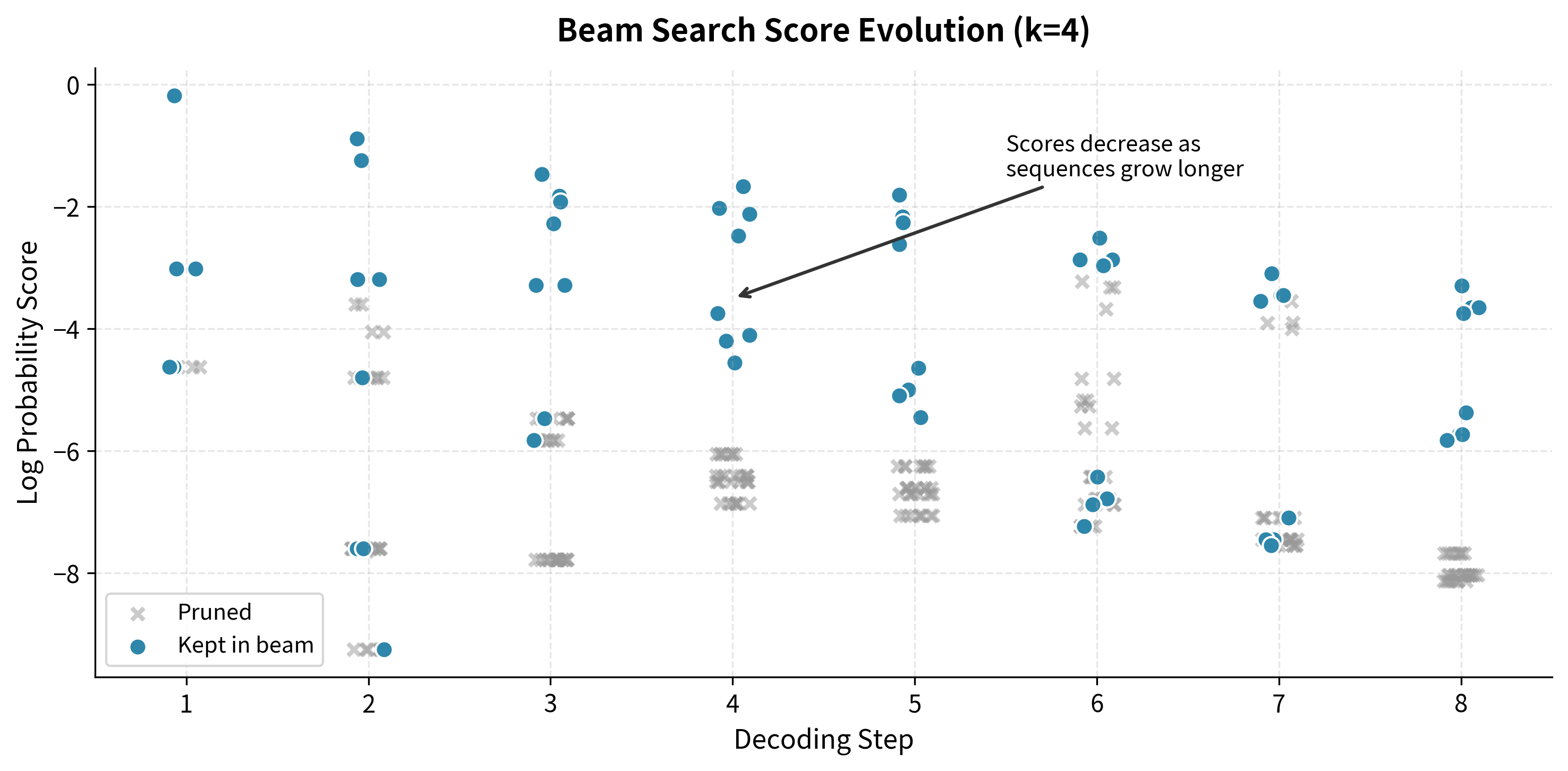
The visualization shows several important dynamics:
- Score decrease: As sequences grow, scores become more negative because each token adds another (negative) log probability term.
- Candidate explosion: At each step, the number of candidates is (beam width × vocabulary size), but only survive.
- Score clustering: Kept hypotheses tend to cluster near the top of the score range, while pruned candidates spread across lower scores.
- Convergence: As decoding progresses, the score gap between kept and pruned candidates often widens as the beam "commits" to promising paths.
Beam Width Selection
The beam width is the primary hyperparameter in beam search. It controls the trade-off between exploration and computational cost.
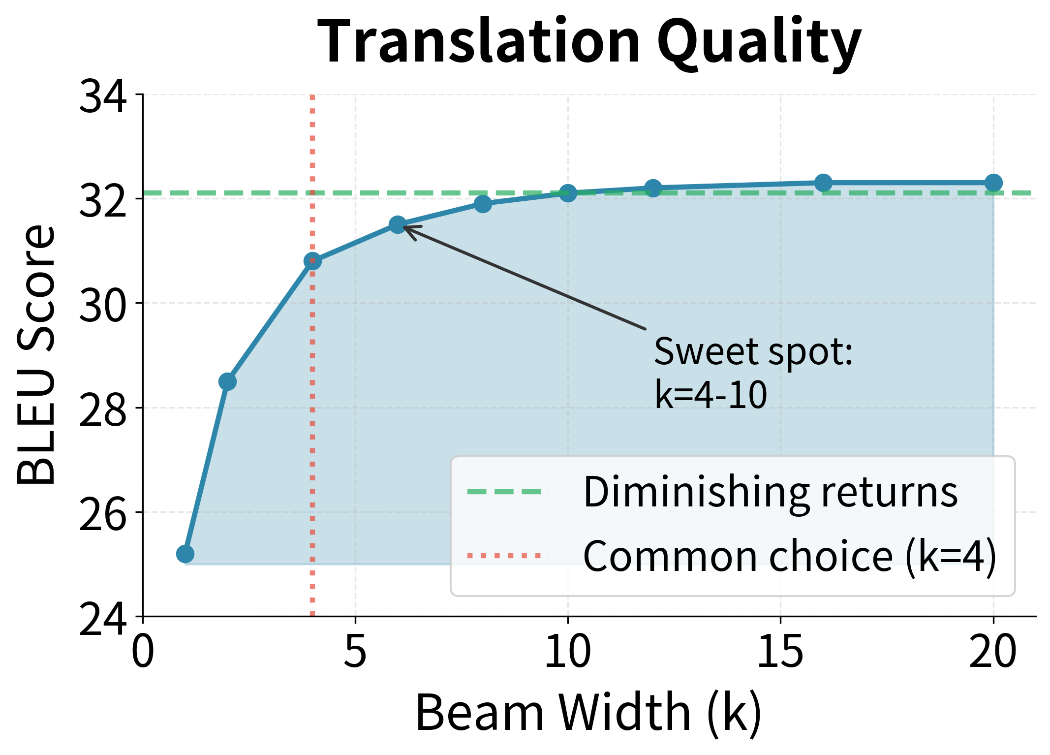
The key observations about beam width are:
- : Equivalent to greedy decoding. Fast but often produces suboptimal sequences.
- to : The sweet spot for most applications. Provides significant quality improvements over greedy decoding with manageable computational overhead.
- : Diminishing returns. Quality improvements become marginal while computation continues to grow linearly.
The optimal beam width depends on the task and model. Machine translation typically uses to . Summarization and dialogue systems might use smaller beams ( to ) since diversity matters more than finding the single best sequence. Speech recognition often uses larger beams ( to ) because the search space is more constrained by acoustic evidence.
With beam width 1 (greedy decoding), we find only one sequence. As beam width increases, we explore more alternatives and may find better-scoring sequences. The best sequence often stabilizes at moderate beam widths, confirming that very large beams provide diminishing returns.
Length Normalization
Our basic beam search implementation has a subtle but significant flaw: it systematically prefers shorter sequences over longer ones, even when the longer sequence is a better output. Understanding why this happens and how to fix it reveals important insights about working with log probabilities.
The Length Bias Problem
Recall that each token contributes a negative log probability to the cumulative score (since for any ). This creates an arithmetic bias: longer sequences accumulate more negative terms, driving their scores lower regardless of quality.
Consider a concrete example:
- Hypothesis A: "The cat sat" with score (3 content tokens)
- Hypothesis B: "The cat sat on the mat" with score (6 content tokens)
Raw beam search prefers Hypothesis A because . But Hypothesis B is clearly a more complete sentence! The problem is that we're comparing apples to oranges: Hypothesis B has made more probabilistic choices, so naturally it has accumulated more "cost."
This isn't a flaw in the math. It's a flaw in what we're optimizing. Raw log probability asks "what's the probability of this exact sequence?" But what we really want is "how good is each token choice, on average?"
The Solution: Normalize by Length
To fairly compare sequences of different lengths, we divide the cumulative score by a function of the sequence length. The normalized score effectively measures average log probability per token rather than total log probability.
The length-normalized score divides the cumulative log probability by , where is the sequence length:
where:
- : the length-normalized score for sequence
- : the length of the generated sequence (number of tokens)
- : the length penalty exponent, typically in the range
- : the normalization factor, which grows with sequence length
- : the raw cumulative log probability (same as the unnormalized score)
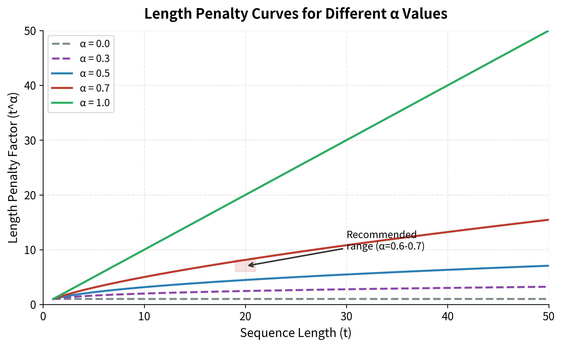
Why the exponent ? The parameter controls how much we compensate for length:
- : No normalization at all. , so we use raw scores. Short sequences are strongly favored.
- : Moderate normalization. We divide by , partially compensating for length.
- : Full normalization. We divide by , computing the average log probability per token. This can over-compensate, sometimes favoring unnecessarily long sequences.
In practice, to works well for most tasks. This provides enough compensation to prevent truncated outputs without encouraging verbose padding.
Visualizing the Effect
The following table demonstrates how length normalization changes which hypothesis "wins." Without normalization, the shortest sequence has the highest (least negative) score. With normalization (), sequences are compared fairly based on their average token quality.
| Sequence | Length | Raw Score | Normalized Score | Winner? |
|---|---|---|---|---|
| Short | 3 | −1.5 | −0.69 | Raw ✓ |
| Medium | 5 | −2.0 | −0.63 | Normalized ✓ |
| Long | 8 | −3.5 | −0.82 | |
| Very Long | 12 | −6.0 | −1.04 |
Task-Specific Tuning
The optimal depends on your task's desired output length:
| Task | Recommended | Reasoning |
|---|---|---|
| Summarization | 0.5 - 0.6 | Shorter outputs are often appropriate |
| Translation | 0.6 - 0.7 | Balance between brevity and completeness |
| Dialogue | 0.7 - 0.8 | Responses should be appropriately detailed |
| Story generation | 0.8 - 1.0 | Longer outputs may be desirable |
Implementation
Adding length normalization to beam search requires only a small modification: instead of sorting candidates by raw score, we sort by normalized score. The key insight is that normalization affects comparison but we still track the raw score for final reporting.
The only change from our basic implementation is the get_normalized_score function and using it as the sort key. This small modification can dramatically improve output quality for tasks where appropriate length matters.
Diverse Beam Search
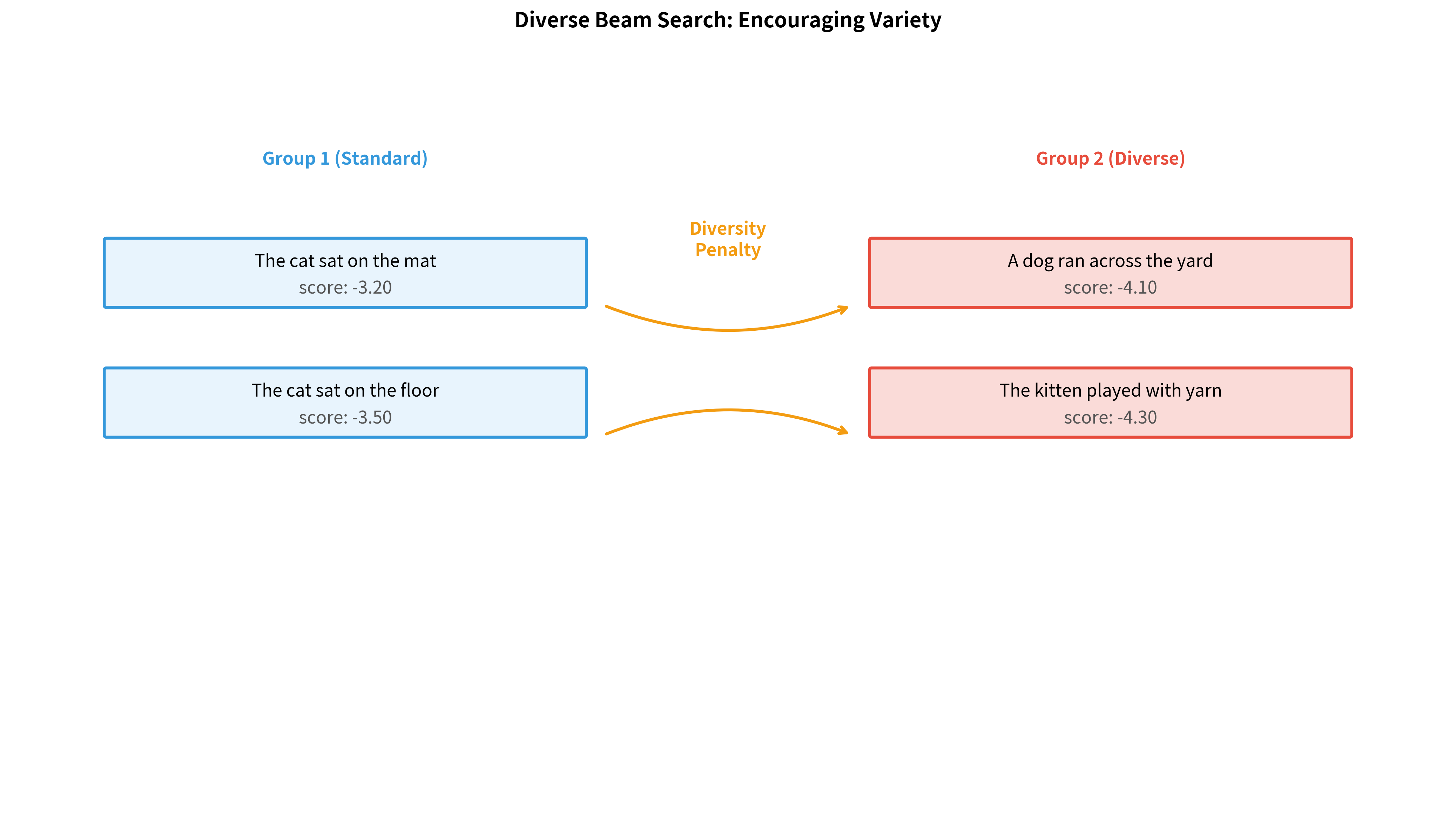
Standard beam search has an unexpected limitation: the hypotheses it returns are often nearly identical. If the top candidate is "The cat sat on the mat," the second and third candidates might be "The cat sat on the floor" and "The cat sat on the rug," differing only in the final word. This happens because beam search greedily pursues high-probability paths, and in natural language, similar beginnings tend to have similar continuations.
For many applications, this lack of diversity is a serious problem:
- Dialogue systems need varied responses to avoid sounding robotic
- Creative writing assistants should offer genuinely different alternatives
- Reranking pipelines benefit from diverse candidates to choose from
Diverse beam search addresses this by explicitly encouraging hypotheses to differ from each other.
The Group-Based Approach
The key idea is to partition the beam into groups, where each group is encouraged to explore different regions of the output space. Group 1 runs standard beam search. Group 2 penalizes hypotheses that are similar to Group 1's selections, pushing it toward different word choices. Group 3 penalizes similarity to both Groups 1 and 2, and so on.
The Algorithm
Diverse beam search modifies the standard algorithm by processing groups sequentially and penalizing similarity:
- Partition the beam into groups, each maintaining hypotheses
- Process Group 1 using standard beam search (no penalty)
- For each subsequent group , when scoring candidates:
- Compute the base score (log probability) as usual
- Subtract a penalty for similarity to hypotheses in groups
- Select the top candidates by this penalized score
- Combine all groups' hypotheses for the final output
The Diversity Penalty
The penalty for hypothesis in group accumulates similarity to all hypotheses selected by earlier groups. The penalized score for a candidate hypothesis is computed by subtracting a diversity term from the base log probability score:
where:
- : the adjusted score for hypothesis when being considered for group
- : the base log probability score of hypothesis (computed as usual)
- : a hyperparameter controlling the strength of diversification (typical values: 0.5 to 1.0; higher values enforce more diversity)
- : iteration over all groups with indices less than (i.e., groups processed earlier)
- : the set of hypotheses selected for group
- : iteration over all hypotheses in group
- : a function measuring overlap between hypotheses and (returns higher values for more similar sequences)
Measuring similarity. Common choices for the similarity function include:
- Hamming distance: Count the number of positions where the two sequences have the same token. Simple and fast.
- N-gram overlap: Count shared bigrams or trigrams. Captures phrase-level similarity.
- Token-level penalty: Penalize selecting the same token at the same position as any previous group's hypothesis.
The effect. By subtracting this penalty from the score, hypotheses that share many tokens with earlier groups become less attractive. Group 2 is pushed away from Group 1's choices; Group 3 is pushed away from both Groups 1 and 2. The result is a diverse set of outputs that collectively cover more of the plausible output space.
Beam Search vs Sampling
Beam search finds high-probability sequences, but high probability doesn't always mean high quality. For creative tasks like story generation or dialogue, the most probable response is often generic and boring. Sampling-based methods introduce randomness to produce more diverse and interesting outputs.
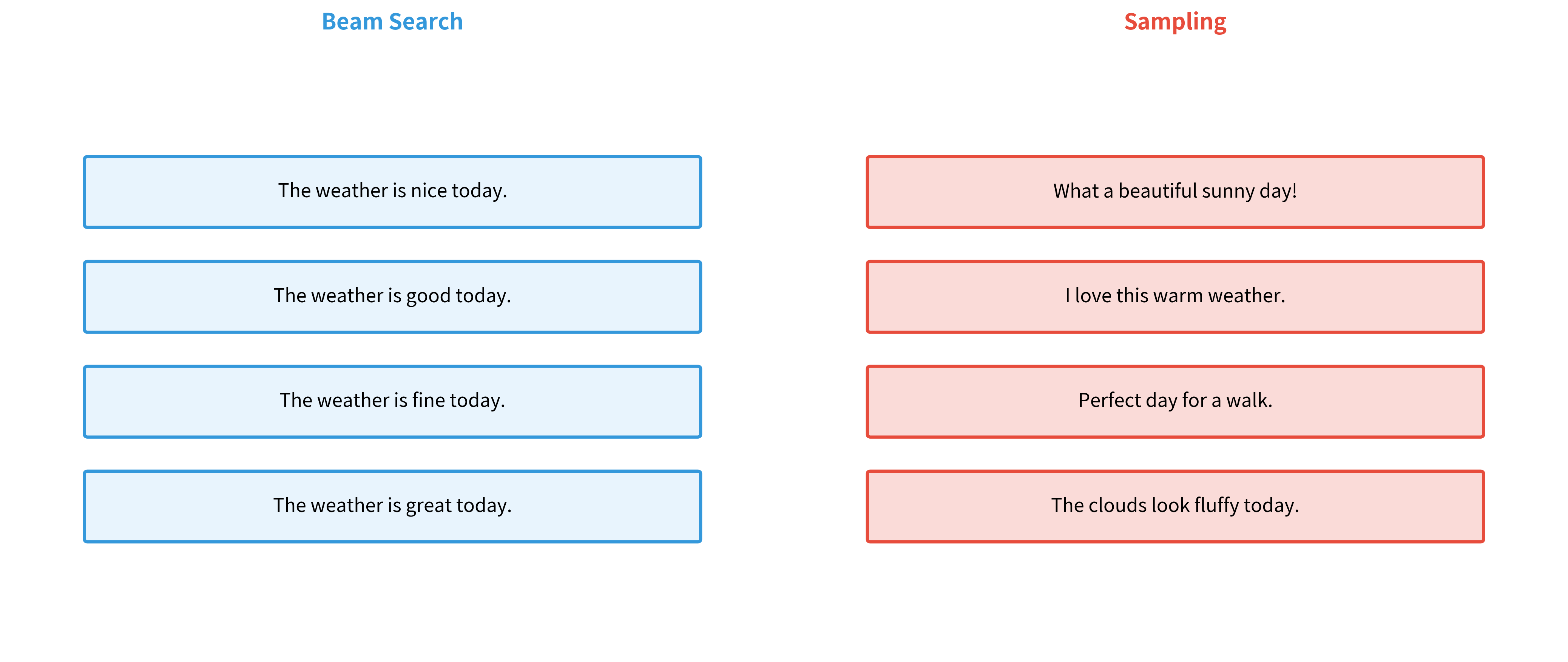
The key sampling methods are:
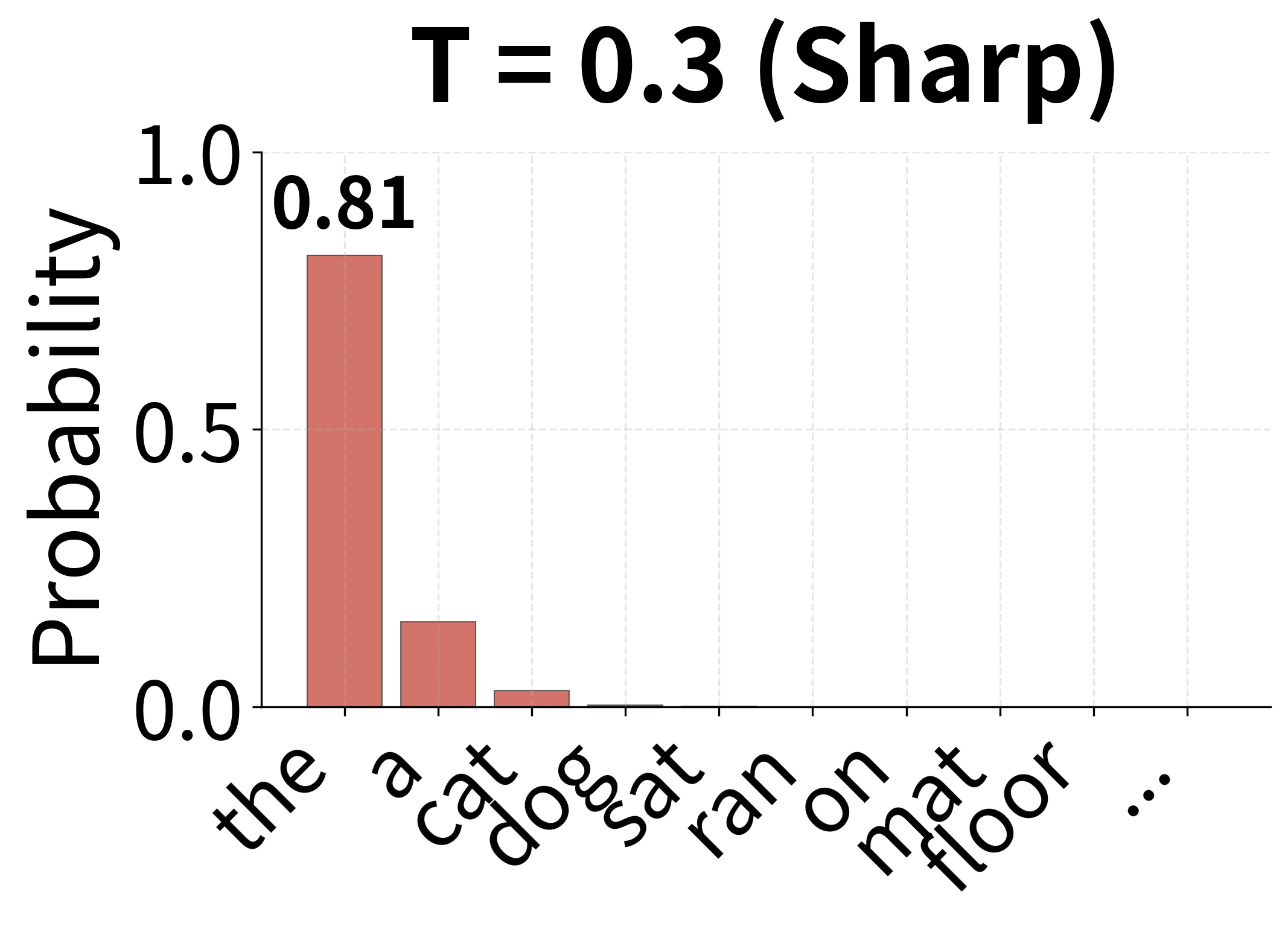
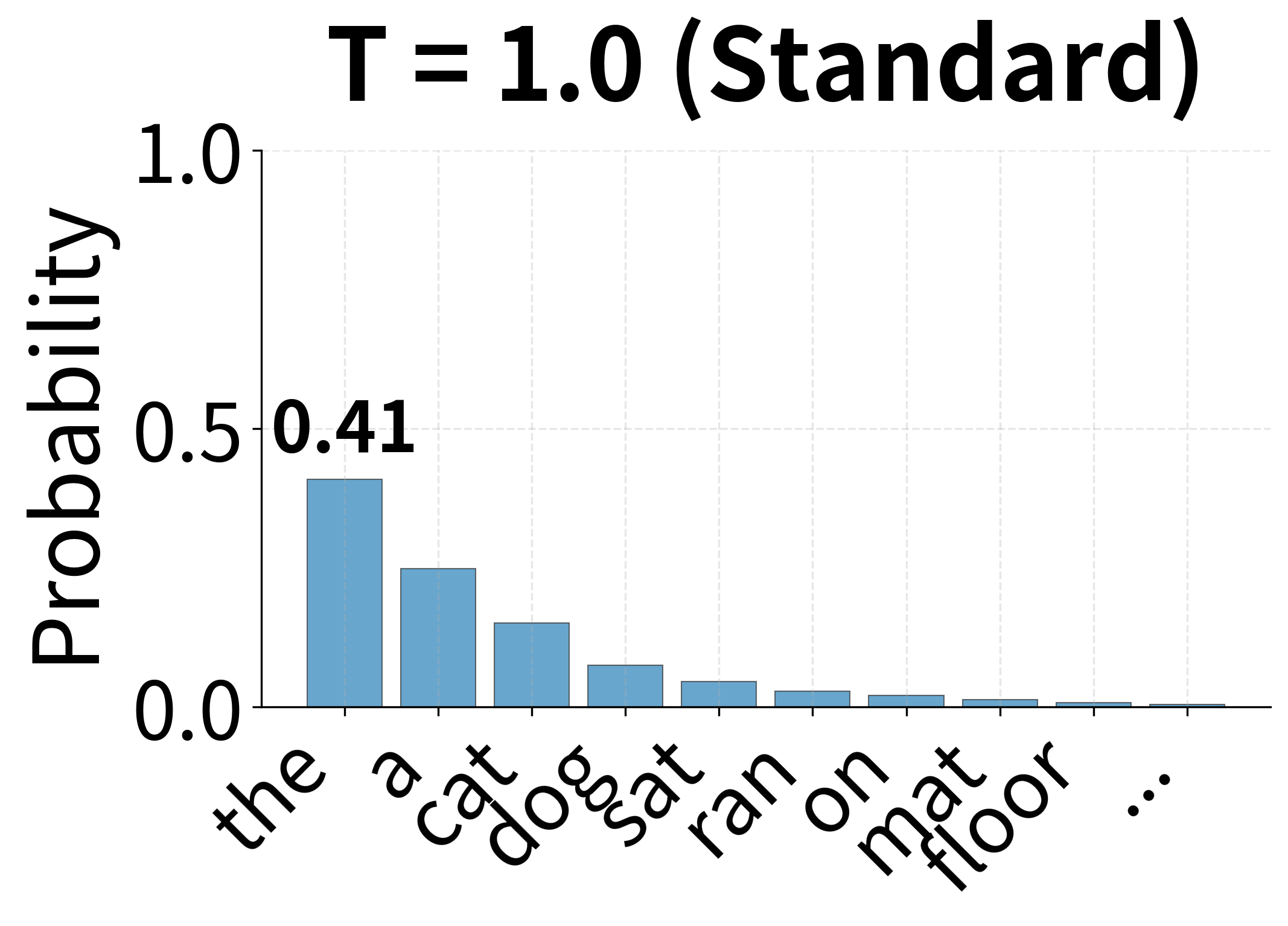
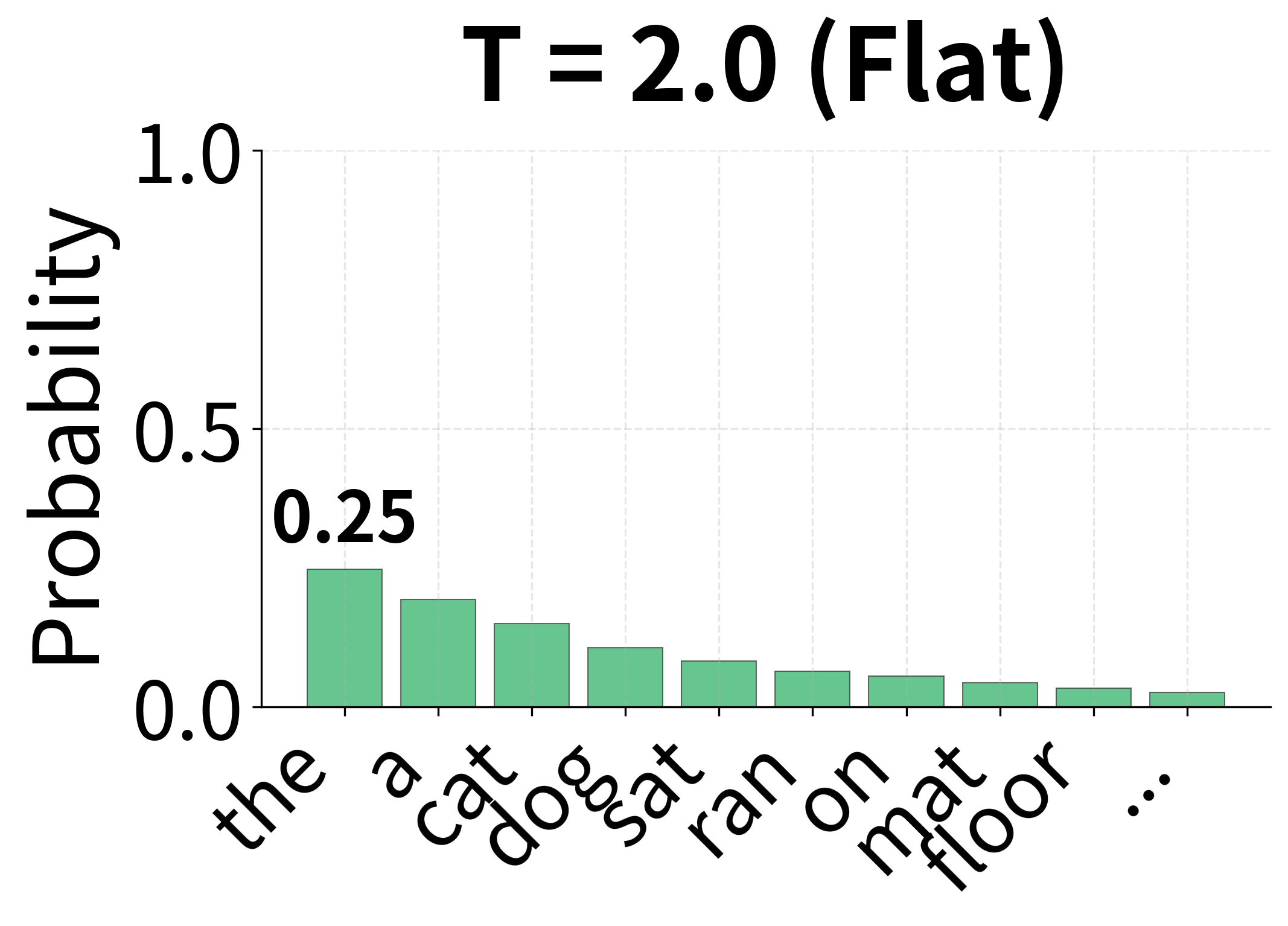
Temperature sampling scales the logits before applying softmax, controlling how "peaked" or "flat" the resulting probability distribution is. The temperature-scaled probability for token is:
where:
- : the probability of selecting token after temperature scaling
- : the logit (unnormalized score) for token from the model's output layer
- : the temperature parameter, a positive real number that controls randomness
- : the vocabulary size (total number of possible tokens)
- : the exponentiated scaled logit, which determines the token's relative weight
- : the normalization constant summing over all vocabulary tokens
Why does temperature work? Dividing by before exponentiation changes the relative differences between logits:
- : Standard softmax. The distribution reflects the model's learned preferences.
- (e.g., 0.5): Dividing by a small number amplifies differences between logits. If and , then and , so the gap widens from 1 to 2. This makes the distribution more peaked, favoring high-probability tokens.
- (e.g., 2.0): Dividing by a large number compresses differences. The same logits become and , so the gap shrinks from 1 to 0.5. This flattens the distribution, giving lower-probability tokens more chance.
In the limit: as , the distribution approaches a one-hot vector (greedy selection of the maximum logit). As , the distribution approaches uniform (random selection).
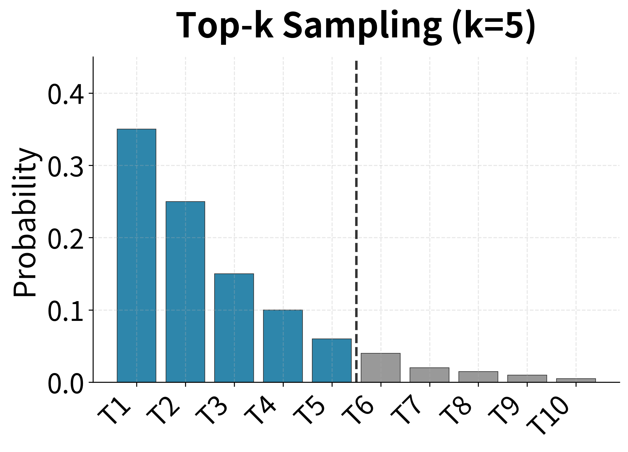
Top-k sampling restricts sampling to the most probable tokens, setting all other probabilities to zero. This prevents sampling very unlikely tokens while maintaining diversity among likely options.
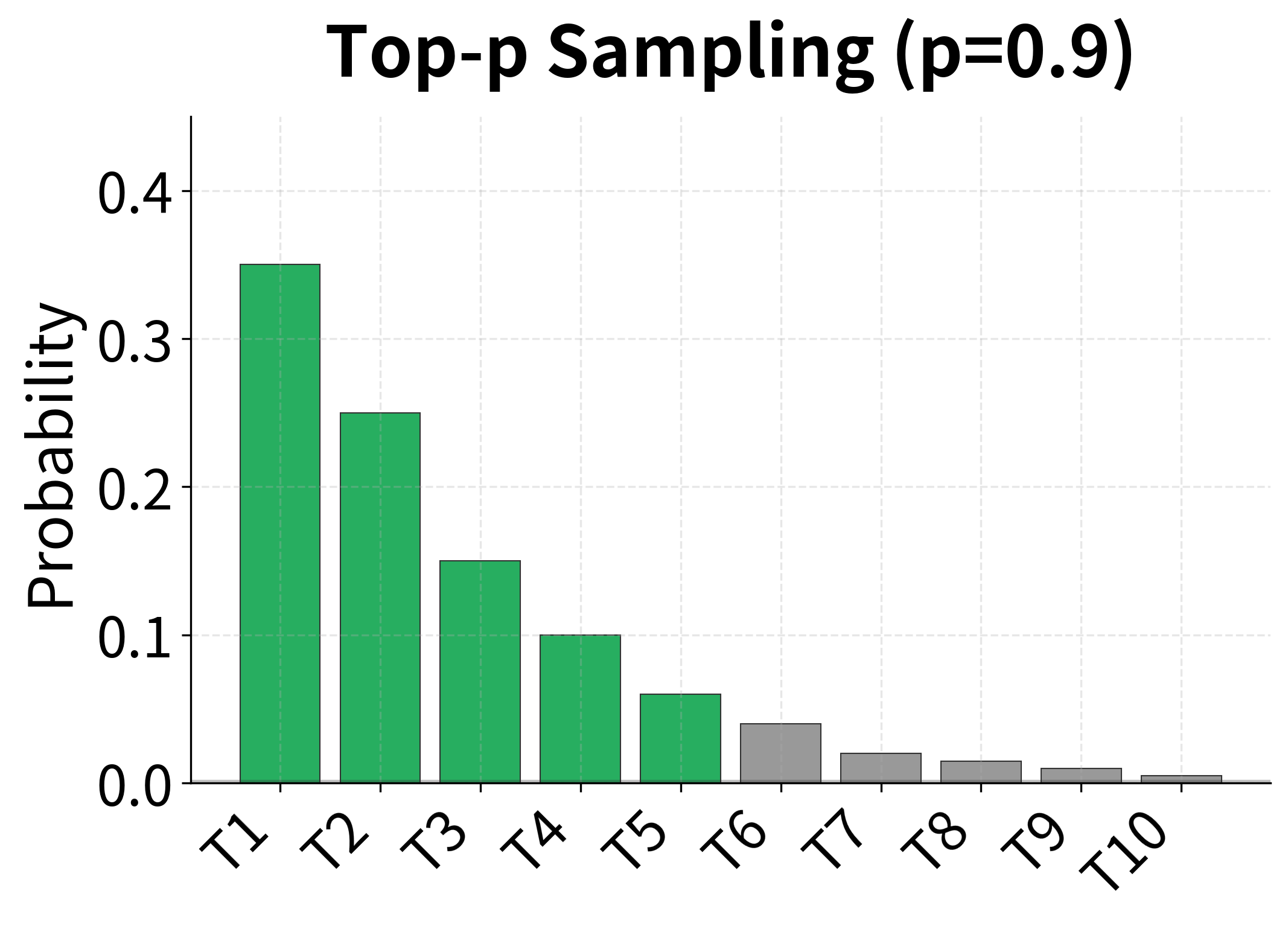
Top-p (nucleus) sampling dynamically selects the smallest set of tokens whose cumulative probability exceeds . This adapts to the distribution's shape: when the model is confident, fewer tokens are considered; when uncertain, more options remain.
The choice between beam search and sampling depends on the application:
| Application | Recommended Method | Reasoning |
|---|---|---|
| Machine Translation | Beam search (k=4-6) | Accuracy matters most; one correct translation needed |
| Summarization | Beam search (k=4) | Faithfulness to source is critical |
| Dialogue Systems | Sampling (top-p=0.9) | Diversity prevents repetitive responses |
| Creative Writing | Sampling (T=0.8-1.2) | Creativity and surprise are valued |
| Code Generation | Beam search or low-T sampling | Correctness is essential |
A Complete Beam Search Implementation
We've now covered all the key concepts: the basic expand-score-prune algorithm, log-space computation, length normalization, and diversity. Let's consolidate these into a production-ready implementation that you could use in real applications.
Design Decisions
A practical beam search decoder needs several features beyond the basic algorithm:
- Length normalization to fairly compare sequences of different lengths
- Minimum length constraints to prevent trivially short outputs
- Early stopping to save computation when enough good hypotheses are found
- N-best output to return multiple candidates for downstream reranking
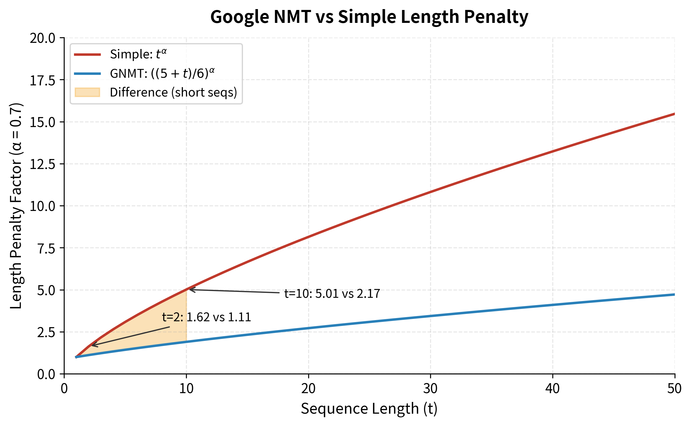
The implementation below uses the length penalty formula from Google's Neural Machine Translation paper. Rather than dividing by directly, it uses a smoothed version that prevents excessive penalty for very short sequences:
where:
- : the length penalty factor for a sequence of length
- : the number of tokens in the sequence
- : the length penalty exponent (same as before, typically 0.6 to 0.7)
- The constants 5 and 6 are chosen so that when , providing a smooth baseline
This formula behaves similarly to for longer sequences but is gentler on short sequences. For example, with : a 2-token sequence gets penalty factor instead of .
Testing the Complete Decoder
Let's verify that our implementation works correctly with the mock language model:
Understanding the output. The decoder returns tuples of (tokens, raw_score). The raw score is the unnormalized cumulative log probability, useful for comparing to other systems or for further processing. The ranking, however, is based on normalized scores internally.
Practical features demonstrated:
- Length normalization: The Google NMT formula provides smoother normalization than simple , especially for short sequences where can be overly aggressive.
- Minimum length enforcement: Hypotheses ending with
<END>before reachingmin_lengthare rejected, preventing degenerate single-word outputs. - Early stopping: Once we have completed hypotheses, we stop expanding, since further search is unlikely to find better candidates.
- N-best output: Returning multiple hypotheses enables downstream reranking with additional models or features.
Limitations and Impact
Beam search has been the dominant decoding algorithm for neural machine translation and other sequence generation tasks since the mid-2010s. Its success stems from finding a practical balance between the exhaustive search (which guarantees finding the optimal sequence but is computationally infeasible) and greedy decoding (which is fast but often suboptimal).
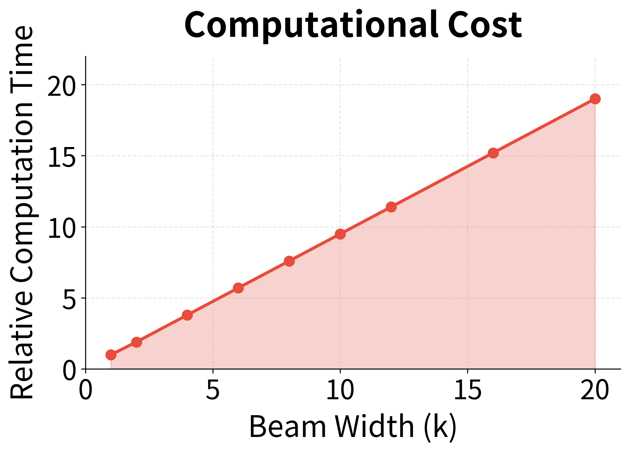
However, beam search has notable limitations. The algorithm is inherently sequential, processing one timestep at a time, which limits parallelization on modern hardware. Each step requires computing probabilities for all vocabulary tokens across all beam hypotheses, making it slower than greedy decoding by a factor roughly equal to the beam width.
More fundamentally, beam search optimizes for probability, not quality. Research has shown that the highest-probability sequence according to a language model isn't always the best output by human judgment. This "probability-quality mismatch" manifests in several ways: beam search can produce generic, repetitive, or overly safe outputs. For open-ended generation tasks like dialogue or creative writing, sampling methods often produce more engaging text despite lower probabilities.
The length bias issue, while addressable through normalization, reveals a deeper problem: sequence-level probability isn't the right objective for many tasks. A sequence might be highly probable because it's short and generic, not because it's a good translation or summary. Length normalization is a heuristic fix rather than a principled solution.
Despite these limitations, beam search remains essential for tasks where accuracy matters more than diversity. Machine translation systems, summarization models, and speech recognition systems all rely heavily on beam search. The algorithm's deterministic nature is actually an advantage in these contexts: given the same input, you get the same output, making systems predictable and debuggable.
The impact of beam search extends beyond its direct applications. The algorithm established the paradigm of maintaining multiple hypotheses during decoding, which influenced later developments like diverse beam search, constrained decoding, and various reranking methods. Understanding beam search is foundational for working with any sequence generation system.
Summary
This chapter explored beam search as a practical algorithm for sequence generation that balances quality against computational cost.
The key concepts covered:
-
Greedy decoding limitations: Selecting the highest-probability token at each step can lead to globally suboptimal sequences because early decisions constrain later options.
-
Beam search algorithm: Maintains candidate hypotheses at each step, expanding all possibilities and pruning to keep the top by cumulative score. This explores multiple paths without the exponential cost of exhaustive search.
-
Log-space computation: Working with log probabilities converts multiplication to addition, preventing numerical underflow and improving computational efficiency.
-
Beam width selection: The beam width controls the exploration-computation trade-off. Values of 4-10 typically provide good results; larger beams offer diminishing returns.
-
Length normalization: Dividing scores by (typically to ) corrects the inherent bias toward shorter sequences.
-
Diverse beam search: Partitioning the beam into groups with diversity penalties encourages exploration of structurally different hypotheses.
-
Beam search vs sampling: Beam search finds high-probability sequences (good for translation, summarization), while sampling methods introduce randomness for more diverse outputs (better for dialogue, creative writing).
The complete beam search procedure, given a model that computes :
- Initialize beam with
<START>token - For each timestep:
-
Expand each hypothesis with all vocabulary tokens
-
Score extensions using cumulative log probability:
-
Optionally apply length normalization:
-
Keep top hypotheses by score
-
Move completed hypotheses (ending with
<END>) to finished list
-
- Return highest-scoring completed hypothesis
In the next chapter, we'll explore attention mechanisms, which address the information bottleneck in encoder-decoder models by allowing the decoder to directly access all encoder states rather than relying on a single context vector.
Key Parameters
When implementing beam search, several parameters significantly impact the quality and efficiency of generated sequences:
-
beam_width (k): The number of hypotheses maintained at each decoding step. Values of 1 reduce to greedy decoding. Values of 4-6 work well for most translation tasks, providing a good balance between quality and speed. Larger values (10-20) may help for speech recognition where acoustic constraints narrow the search space. Increasing beam width improves quality with diminishing returns while linearly increasing computation.
-
max_length: The maximum number of tokens to generate before forcing termination. Set this based on your task's expected output length, typically 1.5-2× the average target length in your training data. Too short truncates valid outputs; too long wastes computation on degenerate sequences.
-
length_penalty (): Controls the strength of length normalization. Values of 0.6-0.7 work well for translation. Lower values (0.5) favor shorter outputs, useful for summarization. Higher values (0.8-1.0) favor longer outputs. Set to 0 to disable length normalization entirely.
-
min_length: The minimum number of tokens required before accepting a completed hypothesis. Prevents the decoder from generating trivially short outputs like single-word responses. Set based on task requirements, typically 5-10 for translation.
-
end_token: The token ID that signals sequence completion. Hypotheses ending with this token are moved to the completed list. Ensure this matches your tokenizer's end-of-sequence token.
-
n_best: The number of top hypotheses to return. Set to 1 for single-best output. Higher values (4-10) enable reranking with additional models or returning multiple alternatives to users.
Quiz
Ready to test your understanding? Take this quick quiz to reinforce what you've learned about beam search and sequence decoding.

Comments