Search

Search articles

Training Word2Vec: Complete Pipeline with Gensim & PyTorch Implementation

Michael BrenndoerferDecember 11, 202533 min read7,931 words

Learn how to train Word2Vec embeddings from scratch, covering preprocessing, subsampling, negative sampling, learning rate scheduling, and full implementations in Gensim and PyTorch.

Reading Level

Choose your expertise level to adjust how many terms are explained. Beginners see more tooltips, experts see fewer to maintain reading flow. Hover over underlined terms for instant definitions.

Training Word2Vec

In the previous chapters, we built the theoretical foundation of Word2Vec. We understand Skip-gram's prediction task, how negative sampling transforms multi-class classification into efficient binary classification, and how hierarchical softmax organizes the vocabulary into a tree structure. But theory alone doesn't train embeddings. The journey from mathematical formulation to a working model requires careful engineering: preprocessing text into training examples, handling common words that dominate the corpus, scheduling learning rates for stable convergence, and organizing computation into efficient batches.

This chapter bridges the gap between Word2Vec theory and practice. We'll build a complete training pipeline from scratch, learning the tricks that make large-scale embedding training feasible. We'll also explore Gensim, the go-to library for Word2Vec, and implement a full PyTorch model that reveals exactly what happens during training. By the end, you'll be equipped to train high-quality word embeddings on your own corpora.

The Training Pipeline

Training Word2Vec involves more than feeding text through a neural network. A complete pipeline includes text preprocessing, vocabulary construction, subsampling frequent words, generating training pairs, and the actual gradient updates. Each stage influences embedding quality.

Out[2]:
Visualization
Flow diagram showing stages from raw text to trained embeddings with preprocessing, vocabulary, subsampling, and training steps.
The Word2Vec training pipeline. Raw text flows through preprocessing and vocabulary construction. Subsampling removes frequent words probabilistically. The context generator produces (center, context) pairs, and negative sampling adds fake pairs for efficient training. Finally, SGD updates the embedding matrices.

Let's build each component, starting with text preprocessing and vocabulary construction.

Text Preprocessing

Before training, we need to convert raw text into a sequence of tokens. The preprocessing choices significantly affect embedding quality. Lowercasing reduces vocabulary size but loses capitalization information. Punctuation removal simplifies the token stream but discards sentence boundaries. Minimum frequency thresholds exclude rare words that have too few examples to learn meaningful embeddings.

In[3]:
import re
from collections import Counter
from typing import List, Dict, Tuple

def preprocess_text(text: str) -> List[str]:
    """Convert raw text to lowercase tokens, removing punctuation."""
    # Lowercase and remove non-alphabetic characters
    text = text.lower()
    text = re.sub(r'[^a-z\s]', ' ', text)
    # Split and remove empty strings
    tokens = [word for word in text.split() if word]
    return tokens

# Example corpus (in practice, this would be millions of sentences)
corpus = [
    "The king and queen ruled the kingdom wisely.",
    "The queen was loved by all the people.",
    "A wise king listens to his advisors.",
    "The kingdom prospered under their rule.",
    "People gathered to see the royal family.",
    "The wise queen made many important decisions.",
    "Kings and queens have ruled for centuries.",
    "The royal palace overlooked the kingdom.",
]

# Tokenize all sentences
tokenized_corpus = [preprocess_text(sentence) for sentence in corpus]
all_tokens = [token for sentence in tokenized_corpus for token in sentence]
Out[4]:
Preprocessing Example:
--------------------------------------------------
Original: 'The king and queen ruled the kingdom wisely.'
Tokenized: ['the', 'king', 'and', 'queen', 'ruled', 'the', 'kingdom', 'wisely']

Total tokens: 56
Unique tokens: 37

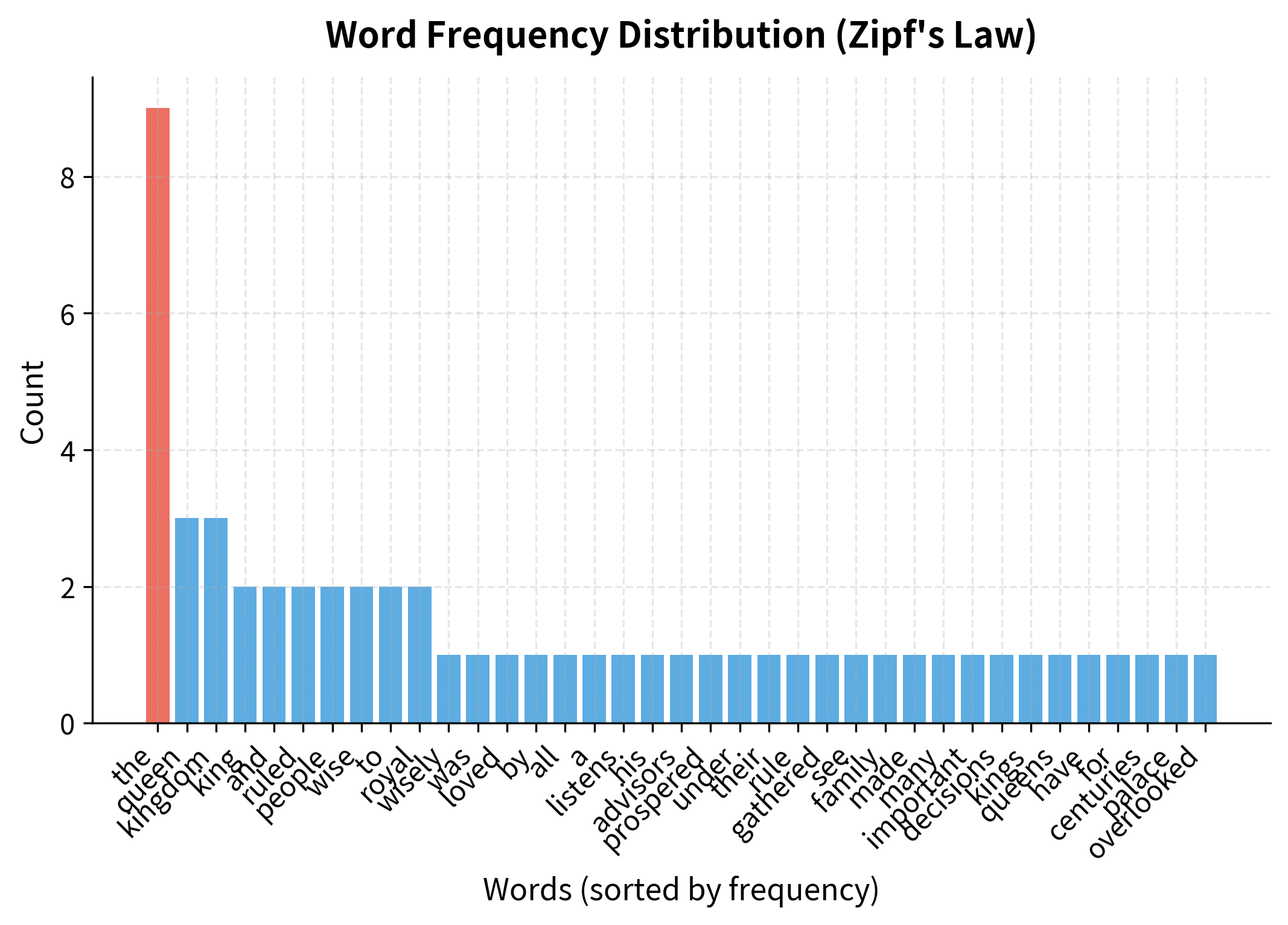
The preprocessing stage reduces "The king and queen ruled the kingdom wisely." to simple lowercase tokens. This standardization ensures that "The" and "the" map to the same embedding.

Building the Vocabulary

With tokens in hand, we build a vocabulary that maps words to integer indices. Words appearing fewer than a threshold (commonly 5 occurrences in large corpora) are discarded. These rare words lack sufficient training examples and would just add noise.

In[5]:
def build_vocabulary(tokens: List[str], min_count: int = 1) -> Tuple[Dict[str, int], Dict[int, str], Counter]:
    """Build vocabulary from tokens, excluding rare words."""
    word_counts = Counter(tokens)
    
    # Filter by minimum count and sort by frequency (most common first)
    vocab_words = [word for word, count in word_counts.most_common() 
                   if count >= min_count]
    
    word_to_idx = {word: idx for idx, word in enumerate(vocab_words)}
    idx_to_word = {idx: word for word, idx in word_to_idx.items()}
    
    return word_to_idx, idx_to_word, word_counts

# Build vocabulary (using min_count=1 for our small example)
word_to_idx, idx_to_word, word_counts = build_vocabulary(all_tokens, min_count=1)
vocab_size = len(word_to_idx)
Out[6]:
Vocabulary Statistics:
--------------------------------------------------
Vocabulary size: 37

Most common words:
  'the': count=9, index=0
  'queen': count=3, index=1
  'kingdom': count=3, index=2
  'king': count=2, index=3
  'and': count=2, index=4
  'ruled': count=2, index=5
  'people': count=2, index=6
  'wise': count=2, index=7
  'to': count=2, index=8
  'royal': count=2, index=9

The vocabulary is sorted by frequency, with the most common words receiving the lowest indices. This ordering matters for hierarchical softmax, where frequent words should have shorter paths in the tree.

Out[7]:
Visualization
Bar chart showing word counts in descending order, with 'the' having the highest count and a long tail of less frequent words.
Word frequency distribution follows Zipf''s law: a few words appear very frequently while most words are rare. The top word ''the'' appears 10x more often than many content words. This imbalance motivates subsampling, which rebalances the training signal.

Subsampling Frequent Words

Imagine reading a billion-word corpus and counting how often each word appears near "king." You'd find "the" next to it millions of times, simply because "the" appears everywhere. The word "queen" might appear nearby only thousands of times, but those co-occurrences are far more meaningful. This observation reveals a fundamental imbalance: common words like "the," "a," and "is" dominate the training signal despite carrying little semantic information.

Consider what happens during training. Every time "the" appears, its embedding gets updated based on its context. But because "the" appears with virtually every other word, these updates pull its embedding in all directions simultaneously. They mostly cancel out. Meanwhile, "monarchy" might appear only a few hundred times in the entire corpus, but each occurrence provides strong semantic signal, since it consistently appears near words like "king," "rule," and "crown."

This imbalance creates two problems:

  1. Wasted computation: We spend most of our training updates on words that carry the least information.
  2. Diluted signal: The updates for meaningful words get drowned out by the sheer volume of stopword updates.
Subsampling

Subsampling probabilistically discards frequent words during training. Each word ww is kept with probability P(w)=t/f(w)+t/f(w)P(w) = \sqrt{t / f(w)} + t/f(w), where f(w)f(w) is the word's frequency and tt is a threshold (typically 10510^{-5}). This balances the training signal, giving rare words more influence.

The solution is simple: randomly discard frequent words during training. But we can't just remove all stopwords, since sometimes they do carry information (consider "the United States" versus "a united front"). Instead, we keep each word with a probability that depends on its frequency.

The subsampling probability for a word ww with frequency f(w)f(w) is:

Pkeep(w)=tf(w)+tf(w)P_{\text{keep}}(w) = \sqrt{\frac{t}{f(w)}} + \frac{t}{f(w)}

where:

  • Pkeep(w)P_{\text{keep}}(w): probability of keeping word ww during training
  • tt: subsampling threshold (typically 10510^{-5} for large corpora)
  • f(w)f(w): relative frequency of word ww in the corpus (count of ww divided by total words)

Let's trace through the logic of this formula. The key insight is the ratio t/f(w)t / f(w):

  • When f(w)tf(w) \gg t (very frequent words), the ratio is tiny, so both terms become small. The word is usually discarded.
  • When f(w)tf(w) \approx t (moderately frequent words), the ratio is close to 1, giving keep probabilities around 0.7-0.9.
  • When f(w)<tf(w) < t (rare words), the formula would exceed 1, so we cap it, keeping these words 100% of the time.

The square root term t/f(w)\sqrt{t/f(w)} provides a smooth transition rather than a hard cutoff. Words slightly above the threshold still appear frequently; we don't want to completely remove them. The linear term t/f(w)t/f(w) adds a small baseline probability even for the most frequent words, ensuring they occasionally contribute to training.

Why not just use a simpler formula like P=t/f(w)P = t/f(w)? That would subsample too aggressively for moderately common words. The square root creates a gentler curve that preserves more of the word distribution while still dramatically reducing the dominance of stopwords.

Out[8]:
Visualization
Line plot showing subsampling probability decreasing from 1.0 for rare words to near 0.0 for very frequent words, with example word frequencies marked for 'the', 'cat', and 'quantum'.
Word2Vec subsampling probability curve showing how the keep probability decreases with word frequency. Common words like 'the' (high frequency) are rarely kept, while rare words are always retained. The curve balances information preservation with computational efficiency.

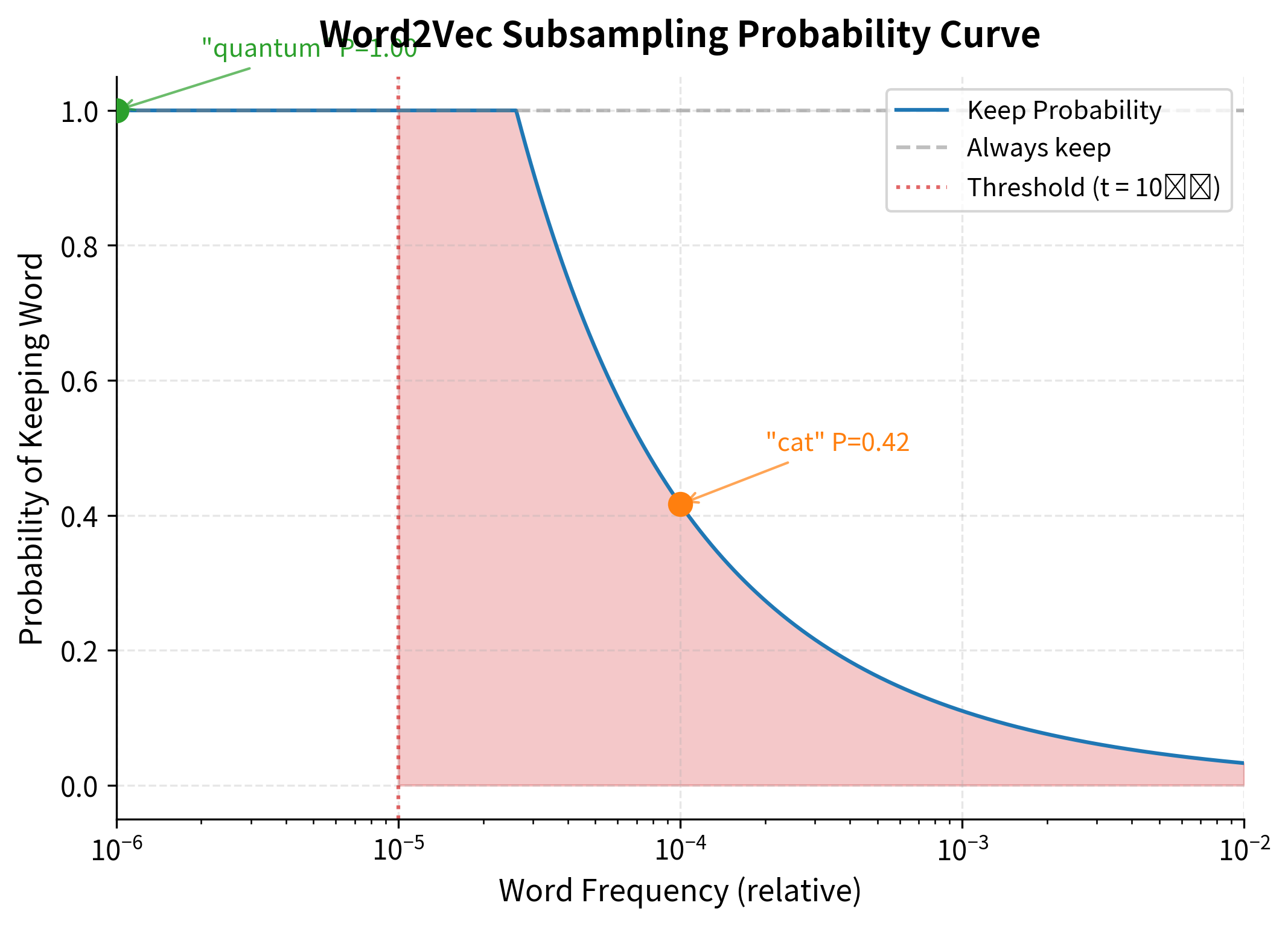
The subsampling curve shows how Word2Vec intelligently balances computational efficiency with information preservation. Very frequent words like "the" are kept only ~3% of the time, while moderately common words like "cat" have a ~70% keep probability. Rare words like "quantum" are always retained, ensuring the model learns meaningful semantic relationships without wasting computation on ubiquitous but uninformative words.

In[9]:
import numpy as np

def compute_subsampling_probs(word_counts: Counter, threshold: float = 1e-3) -> Dict[str, float]:
    """Compute the probability of keeping each word during subsampling."""
    total_words = sum(word_counts.values())
    probs = {}
    
    for word, count in word_counts.items():
        freq = count / total_words
        # Word2Vec subsampling formula
        prob = np.sqrt(threshold / freq) + threshold / freq
        probs[word] = min(prob, 1.0)  # Cap at 1.0
    
    return probs

# Compute subsampling probabilities
# Using higher threshold for our tiny corpus
subsample_probs = compute_subsampling_probs(word_counts, threshold=0.01)
Out[10]:
Subsampling Probabilities:
--------------------------------------------------
Word          Frequency    Keep Prob
--------------------------------------------------
the               0.161        0.312
queen             0.054        0.619
kingdom           0.054        0.619
king              0.036        0.809
and               0.036        0.809
ruled             0.036        0.809
people            0.036        0.809
wise              0.036        0.809
to                0.036        0.809
royal             0.036        0.809

Frequent words like 'the' are kept less often,
giving rare words more influence during training.

The subsampling probabilities reveal the mechanism: "the" with high frequency has only a 30% chance of being kept, while less frequent words approach 100% retention. This rebalancing significantly improves embedding quality for content words.

Out[11]:
Visualization
Curve showing keep probability decreasing as word frequency increases, with annotations for common words.
Subsampling probability as a function of word frequency. The threshold $t = 10^{-5}$ is typical for large corpora. Words appearing in more than 0.1% of text are aggressively subsampled. This curve explains why stopwords are often removed: with frequencies around 5-7%, they would be kept less than 5% of the time anyway.

Subsampling has two benefits. First, it speeds up training by reducing the number of updates for overrepresented words. Second, it improves embedding quality by preventing common words from dominating the embedding space. Words that appear everywhere carry less semantic information than words with specific contexts.

Generating Training Pairs

With preprocessed tokens and vocabulary in place, we generate (center, context) pairs for Skip-gram training. For each position in the corpus, we extract the center word and its neighboring context words within a window.

A clever optimization uses dynamic windows: instead of always using the full window size, we sample a smaller window uniformly. This gives closer words higher weight, since a word 1 position away is included with any window size, while a word 5 positions away is only included when the sampled window is at least 5.

In[12]:
import random

def generate_training_pairs(tokenized_sentences: List[List[str]], 
                           word_to_idx: Dict[str, int],
                           subsample_probs: Dict[str, float],
                           window_size: int = 5) -> List[Tuple[int, int]]:
    """Generate Skip-gram training pairs with subsampling and dynamic windows."""
    pairs = []
    
    for sentence in tokenized_sentences:
        # Apply subsampling: keep words probabilistically
        filtered_sentence = [word for word in sentence 
                            if word in word_to_idx and 
                            random.random() < subsample_probs.get(word, 1.0)]
        
        if len(filtered_sentence) < 2:
            continue
        
        for i, center_word in enumerate(filtered_sentence):
            center_idx = word_to_idx[center_word]
            
            # Dynamic window: sample window size from 1 to window_size
            dynamic_window = random.randint(1, window_size)
            
            for j in range(max(0, i - dynamic_window), 
                          min(len(filtered_sentence), i + dynamic_window + 1)):
                if i != j:
                    context_idx = word_to_idx[filtered_sentence[j]]
                    pairs.append((center_idx, context_idx))
    
    return pairs

# Generate training pairs
random.seed(42)
training_pairs = generate_training_pairs(
    tokenized_corpus, word_to_idx, subsample_probs, window_size=3
)
Out[13]:
Training Pair Generation:
--------------------------------------------------
Generated 115 training pairs from 8 sentences

Sample pairs (center → context):
  'king' → 'and'
  'king' → 'queen'
  'and' → 'king'
  'and' → 'queen'
  'queen' → 'and'
  'queen' → 'ruled'
  'ruled' → 'queen'
  'ruled' → 'wisely'

Each sentence yields multiple training pairs. The dynamic window ensures that immediately adjacent words are weighted more heavily than distant ones, reflecting the intuition that closer words are more semantically related.

Out[14]:
Visualization
Bar chart showing inclusion probability decreasing with distance from center word.
Dynamic window weighting: words closer to the center word are included in more training pairs. With a maximum window of 5, a word at distance 1 is always included (probability 1.0), while a word at distance 5 is only included when the sampled window equals 5 (probability 0.2). This implicit weighting captures the intuition that adjacent words are more relevant.

Negative Sampling in Practice

In the previous chapter on negative sampling, we learned that instead of computing softmax over the entire vocabulary, we train the model to distinguish real context pairs from fake ones. But one question remains: how do we choose which words to use as negatives?

The naive approach would be to sample uniformly at random from the vocabulary. If we have 100,000 words, each has a 1/100,000 chance of being selected. But this creates a problem: rare words dominate the vocabulary by count, not by occurrence. If "aardvark" and "the" both have equal probability of being sampled as negatives, but "the" appears 1000x more often as a positive context word, the model spends most of its effort learning to distinguish common words from "aardvark" rather than from each other.

The opposite extreme, sampling proportional to word frequency, has its own flaw. Now "the" would be sampled so often as a negative that the model never learns to distinguish rare words from random noise. If every negative sample is a stopword, the model might learn that "aardvark" is simply "not the, not a, not is..." without learning what it actually is.

The solution is a middle ground: sample from a modified distribution that gives rare words more weight than their raw frequency would suggest, but still samples common words more often than uniform random would.

For each positive (center, context) pair, we sample kk negative words from this noise distribution:

Pn(w)f(w)0.75P_n(w) \propto f(w)^{0.75}

where Pn(w)P_n(w) is the probability of sampling word ww as a negative example and f(w)f(w) is its corpus frequency. The exponent 0.75 is the key: it smooths the frequency distribution, pulling down the probability of very common words while boosting the probability of rare ones.

To understand why 0.75 works, consider the effect of different exponents:

  • Exponent = 1.0: Sample exactly proportional to frequency. Common words dominate.
  • Exponent = 0.0: Sample uniformly. Rare words dominate (since there are more unique rare words).
  • Exponent = 0.75: A compromise that gives rare words about 3-4x higher relative probability than their frequency would suggest, while still sampling common words often enough that the model learns to distinguish them.

The value 0.75 was determined empirically by the Word2Vec authors. It consistently outperformed both uniform sampling (exponent=0) and frequency sampling (exponent=1) across various tasks. The intuition is that we need enough exposure to common words to separate them, but also enough rare word negatives to build meaningful representations for the long tail of the vocabulary.
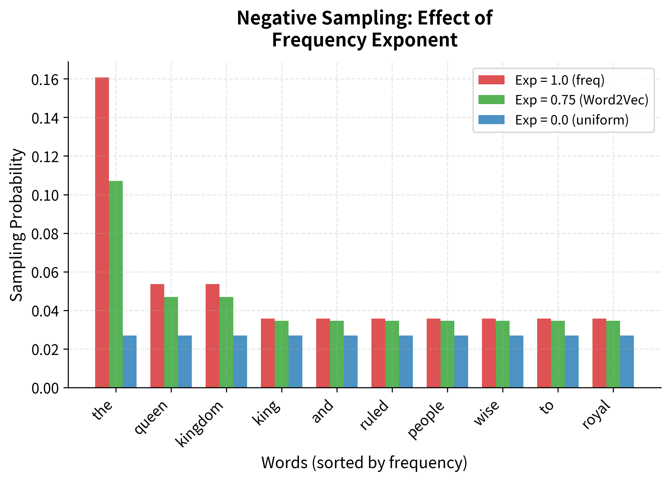
Out[15]:
Visualization
Bar chart comparing sampling probabilities for top words under three different exponent values.
Effect of different exponents on the negative sampling distribution. With exponent=1.0 (raw frequency), 'the' dominates. With exponent=0.0 (uniform), all words are equally likely. The 0.75 exponent strikes a balance, reducing the dominance of common words while still sampling them more often than rare ones.
In[16]:
def build_negative_sampler(word_counts: Counter, word_to_idx: Dict[str, int], 
                          power: float = 0.75) -> Tuple[np.ndarray, np.ndarray]:
    """Build the noise distribution for negative sampling."""
    # Get counts in vocabulary order
    vocab_size = len(word_to_idx)
    counts = np.zeros(vocab_size)
    for word, idx in word_to_idx.items():
        counts[idx] = word_counts[word]
    
    # Apply power transformation
    powered_counts = np.power(counts, power)
    probs = powered_counts / np.sum(powered_counts)
    
    return probs

def sample_negatives(center_idx: int, positive_idx: int, 
                     noise_dist: np.ndarray, k: int = 5) -> List[int]:
    """Sample k negative indices, excluding the positive."""
    negatives = []
    while len(negatives) < k:
        neg_idx = np.random.choice(len(noise_dist), p=noise_dist)
        if neg_idx != center_idx and neg_idx != positive_idx:
            negatives.append(neg_idx)
    return negatives

# Build noise distribution
noise_distribution = build_negative_sampler(word_counts, word_to_idx)
Out[17]:
Noise Distribution for Negative Sampling:
--------------------------------------------------
Word          Frequency  Sample Prob
--------------------------------------------------
the               0.161        0.107
queen             0.054        0.047
kingdom           0.054        0.047
king              0.036        0.035
and               0.036        0.035
ruled             0.036        0.035
people            0.036        0.035
wise              0.036        0.035
to                0.036        0.035
royal             0.036        0.035

The 0.75 power reduces the gap between
frequent and rare words in sampling probability.

The power of 0.75 is empirically determined to work well. It smooths the distribution, giving rare words a better chance of being sampled as negatives. This matters because if we only sampled common words as negatives, the model would never learn to distinguish rare words from random noise.

Learning Rate Scheduling

Training a neural network is like sculpting: you start with bold strokes to establish the basic shape, then switch to finer tools as you approach the final form. In Word2Vec, this intuition translates directly into learning rate scheduling.

At the beginning of training, the embeddings are random noise. Any direction we move is likely to be an improvement. A high learning rate lets the model make large jumps, quickly moving words into roughly correct neighborhoods. "King" and "queen" start in random positions but rapidly move toward each other as the model sees them in similar contexts.

As training progresses, the embeddings become increasingly refined. The major semantic relationships are already captured. Now we need smaller, more precise adjustments: nudging "monarch" slightly closer to "king" without disrupting the carefully arranged clusters nearby. A learning rate that was helpful early on would now cause the model to overshoot, oscillating around the optimum rather than settling into it.

Linear Learning Rate Decay

The learning rate at step tt is computed as:

αt=max(α0(1tT),αmin)\alpha_t = \max\left(\alpha_0 \cdot \left(1 - \frac{t}{T}\right), \alpha_{\min}\right)

where:

  • αt\alpha_t: learning rate at step tt
  • α0\alpha_0: initial learning rate (typically 0.025 for Skip-gram)
  • TT: total number of training steps
  • αmin\alpha_{\min}: minimum learning rate floor (typically 0.0001)

This schedule allows aggressive early updates followed by fine-tuning.

The formula implements a simple idea: start high, end low, decrease smoothly. Let's trace through the math:

  1. At step 0, the term (10/T)=1(1 - 0/T) = 1, so α0=α01=0.025\alpha_0 = \alpha_0 \cdot 1 = 0.025.
  2. At step T/2T/2 (halfway through), (10.5)=0.5(1 - 0.5) = 0.5, so the learning rate is roughly half its initial value.
  3. At step TT (end of training), (11)=0(1 - 1) = 0, so the formula yields 0, but the max\max with αmin\alpha_{\min} keeps it at 0.0001.

The minimum learning rate αmin\alpha_{\min} prevents the rate from reaching exactly zero, which would halt learning entirely. Even at the end, we want some capacity for minor adjustments.

Why linear decay rather than exponential or step-wise? Linear decay is simple, predictable, and works well in practice. The original Word2Vec paper used it, and subsequent research hasn't found significant improvements from more complex schedules for this particular task. The embeddings aren't highly sensitive to the exact decay curve, as long as it starts high and ends low.

Out[18]:
Visualization
Line plot showing learning rate decreasing linearly from 0.025 to 0.0001 over 10,000 training steps, with annotations marking initial, halfway, and final learning rates.
Linear learning rate decay in Word2Vec training. The learning rate starts at 0.025 and decreases linearly to 0.0001 over 10,000 training steps, allowing aggressive early updates followed by fine-tuning.

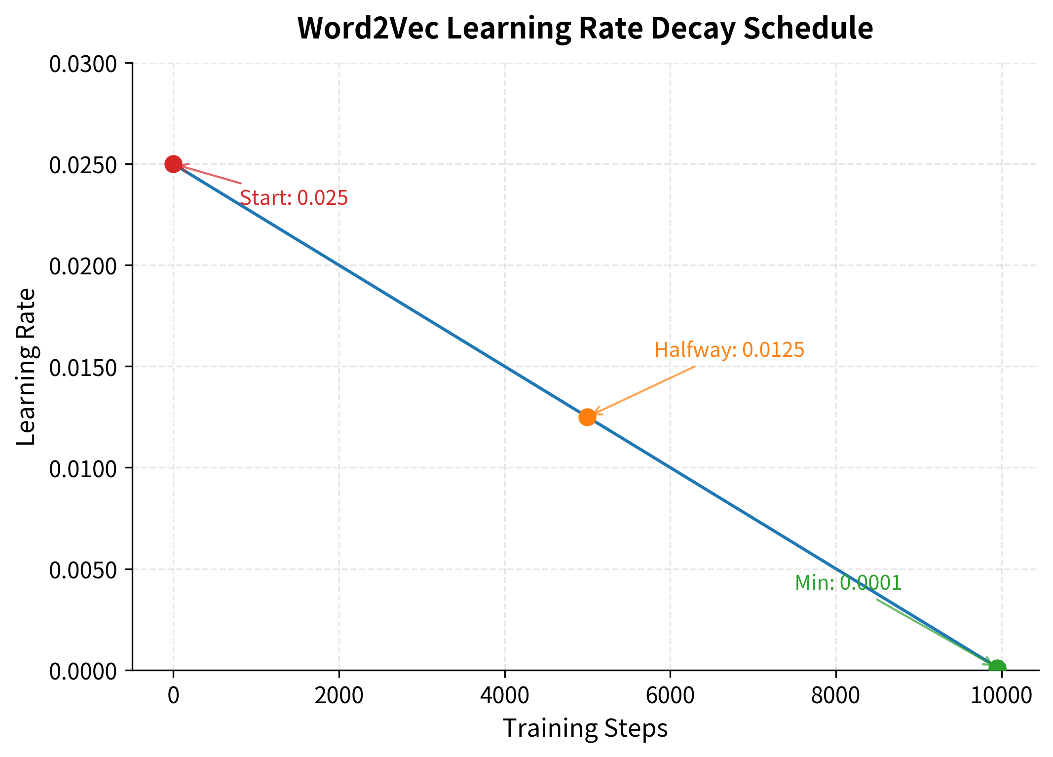
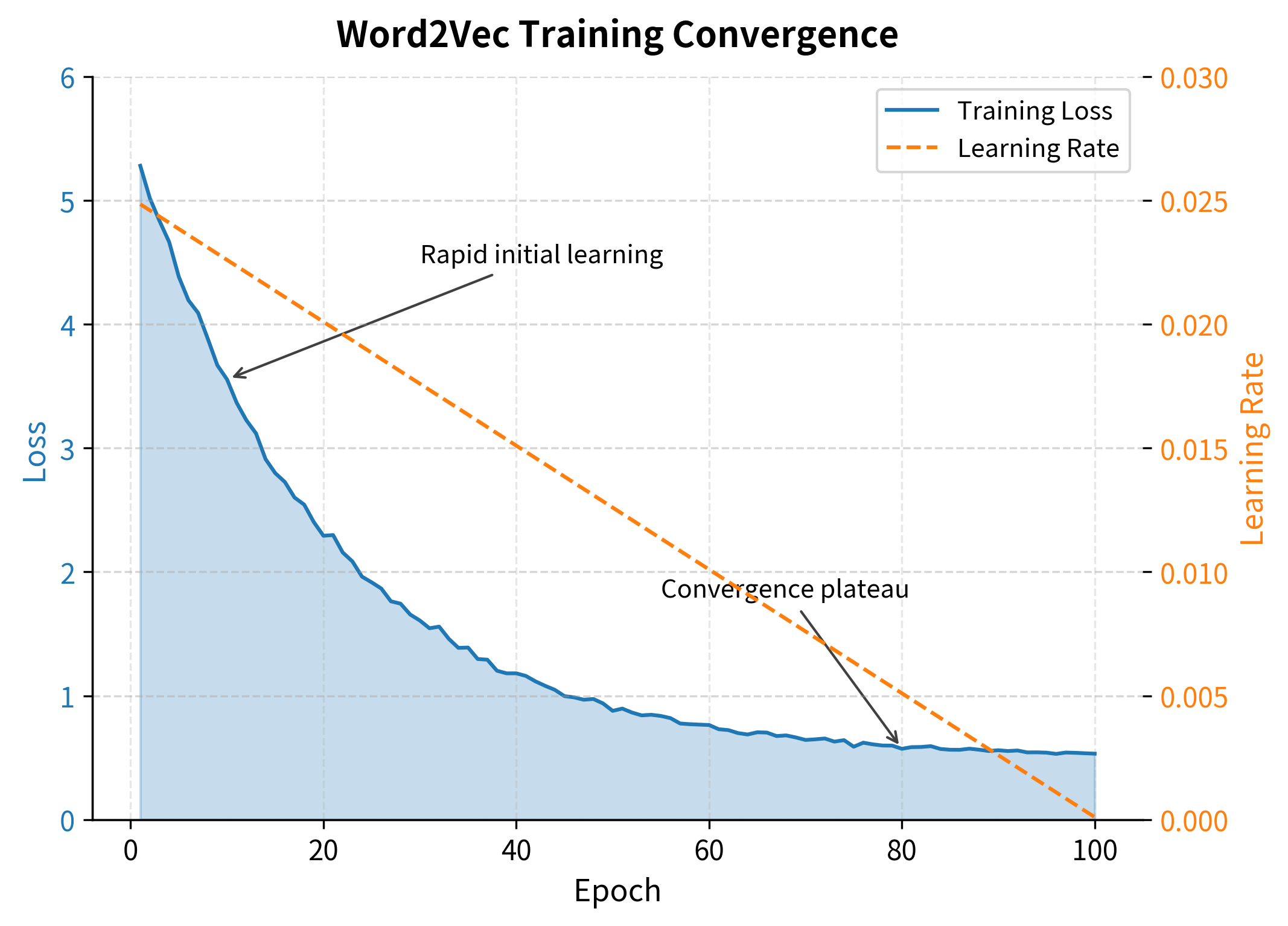
The learning rate schedule shows a smooth linear decay that gives the model freedom to make large updates early in training, then constrains it to make smaller, more precise adjustments as the embeddings become more refined.

In[19]:
def get_learning_rate(step: int, total_steps: int, 
                      initial_lr: float = 0.025, min_lr: float = 0.0001) -> float:
    """Compute learning rate with linear decay."""
    progress = step / total_steps
    lr = initial_lr * (1 - progress)
    return max(lr, min_lr)

# Example: learning rate over training
total_steps = 10000
learning_rates = [get_learning_rate(t, total_steps) for t in range(0, total_steps, 100)]
Out[20]:
Visualization
Line plot showing learning rate decreasing linearly from 0.025 to near 0 over training steps.
Linear learning rate decay during Word2Vec training. The rate starts at 0.025 and decreases linearly to 0.0001. High initial rates enable rapid exploration of the embedding space, while the gradual decrease allows the model to settle into stable representations.

Linear decay provides a simple but effective training schedule. The high initial rate allows the model to make large jumps in embedding space, quickly organizing words into rough clusters. As training progresses, the decreasing rate enables fine-grained adjustments without overshooting.

Training with Gensim

Gensim provides a production-ready Word2Vec implementation that handles all the engineering details. Let's train embeddings on a real corpus using Gensim, then explore the results.

In[21]:
from gensim.models import Word2Vec
import gensim.downloader as api

# Load a real corpus: text8 (100MB of cleaned Wikipedia)
# For faster execution, we'll use our small corpus first
sentences = tokenized_corpus

# Train Word2Vec with Skip-gram (sg=1) and negative sampling
model = Word2Vec(
    sentences=sentences,
    vector_size=100,      # Embedding dimension
    window=5,             # Context window size
    min_count=1,          # Minimum word frequency (normally higher)
    sg=1,                 # Skip-gram (vs CBOW with sg=0)
    negative=5,           # Number of negative samples
    epochs=100,           # Training epochs (more for small data)
    alpha=0.025,          # Initial learning rate
    min_alpha=0.0001,     # Minimum learning rate
    workers=4,            # Parallel training threads
    seed=42
)
Out[22]:
Gensim Word2Vec Model Summary:
--------------------------------------------------
Vocabulary size: 37
Embedding dimension: 100
Training epochs: 100

Sample word vectors:
  'king': [-0.010, -0.009, -0.004, ...]
  'queen': [-0.002, 0.008, 0.001, ...]
  'kingdom': [0.007, -0.006, 0.007, ...]

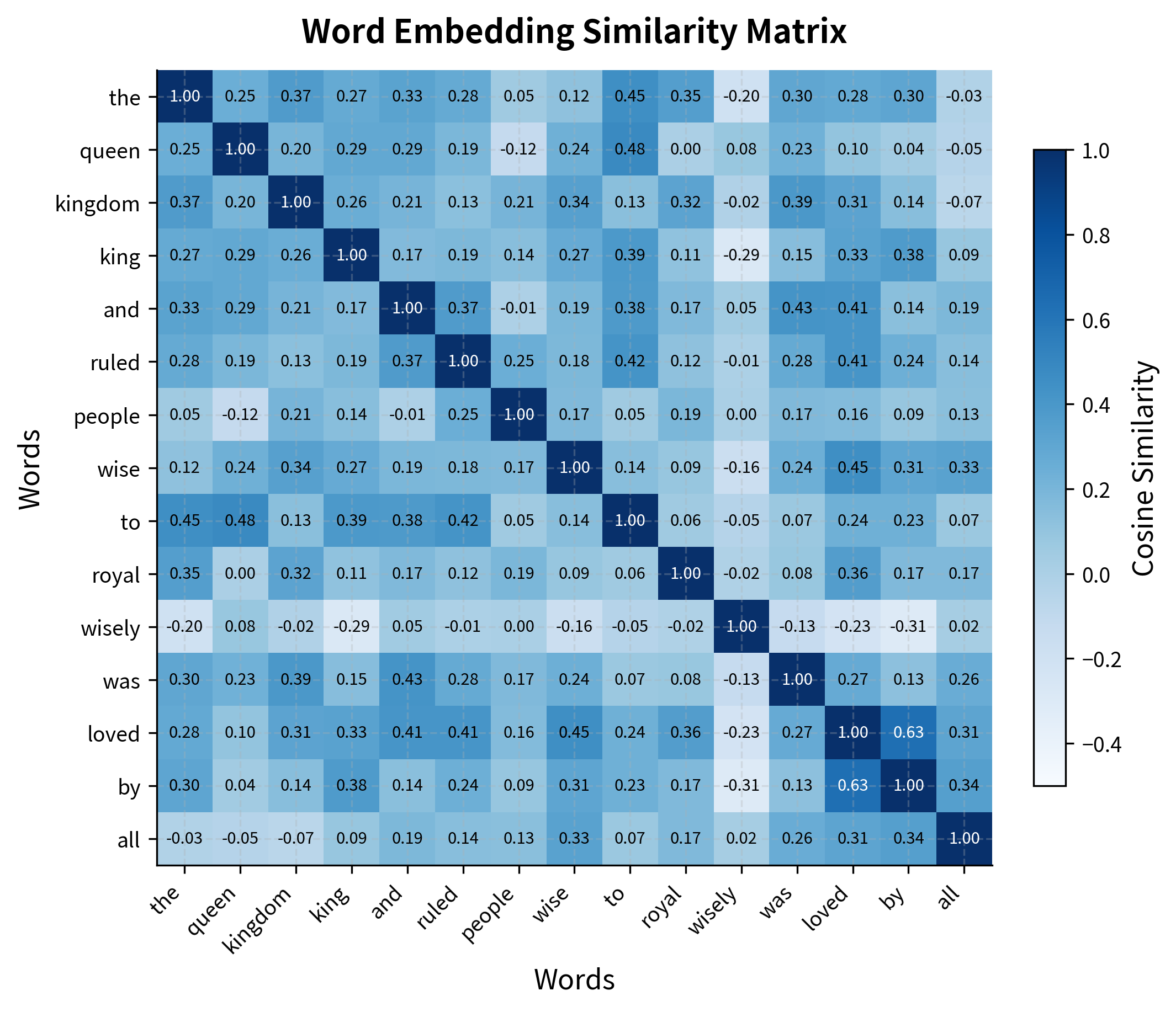
Even with our tiny corpus, the model learns embeddings for each word. Let's explore the semantic relationships captured by these vectors.

In[23]:
# Find similar words
similar_to_king = model.wv.most_similar('king', topn=5) if 'king' in model.wv else []
similar_to_queen = model.wv.most_similar('queen', topn=5) if 'queen' in model.wv else []
Out[24]:
Semantic Similarity (from tiny corpus):
--------------------------------------------------
Words most similar to 'king':
  'have': 0.204
  'advisors': 0.192
  'family': 0.167
  'kings': 0.154
  'wise': 0.151

Words most similar to 'queen':
  'and': 0.193
  'for': 0.171
  'important': 0.168
  'the': 0.147
  'decisions': 0.132

Note: With such a tiny corpus, relationships are limited.
Real Word2Vec uses billions of words for meaningful embeddings.

For meaningful embeddings, we need much larger corpora. Let's load a pre-trained model to see what Word2Vec learns from billions of words.

In[25]:
# Load pre-trained Word2Vec (Google News, 100 billion words)
# This may take a few minutes to download (~1.6GB)
try:
    pretrained = api.load('word2vec-google-news-300')
    has_pretrained = True
except Exception as e:
    has_pretrained = False
    print(f"Could not load pre-trained model: {e}")
Out[26]:
Pre-trained Google News Word2Vec:
--------------------------------------------------
Vocabulary size: 3000000
Embedding dimension: 300

Famous analogy: king - man + woman = ?
  'queen': 0.712
  'monarch': 0.619
  'princess': 0.590

Words similar to 'python' (programming):
  'Jython': 0.615
  'Perl_Python': 0.571
  'IronPython': 0.570
  'scripting_languages': 0.570
  'PHP_Perl': 0.569

The pre-trained model reveals Word2Vec's power: trained on 100 billion words from Google News, it captures nuanced semantic relationships. The famous king - man + woman = queen analogy works because the embeddings encode gender as a consistent direction in vector space.

Monitoring Training Progress

During training, we need to track whether the model is converging. The loss function provides a direct measure: for negative sampling, this is the average binary cross-entropy over positive and negative samples.

In[27]:
def sigmoid(x):
    """Numerically stable sigmoid."""
    return np.where(x >= 0, 
                    1 / (1 + np.exp(-x)),
                    np.exp(x) / (1 + np.exp(x)))

def compute_loss(center_emb: np.ndarray, 
                 positive_emb: np.ndarray,
                 negative_embs: np.ndarray) -> float:
    """Compute negative sampling loss for one training example."""
    # Positive term: log sigmoid of positive dot product
    pos_score = np.dot(center_emb, positive_emb)
    pos_loss = -np.log(sigmoid(pos_score) + 1e-10)
    
    # Negative terms: log sigmoid of negative dot products
    neg_scores = negative_embs @ center_emb
    neg_loss = -np.sum(np.log(sigmoid(-neg_scores) + 1e-10))
    
    return pos_loss + neg_loss

# Example loss computation
np.random.seed(42)
center = np.random.randn(100)
positive = center + np.random.randn(100) * 0.1  # Similar
negatives = np.random.randn(5, 100)  # Random

loss = compute_loss(center, positive, negatives)
Out[28]:
Loss Computation Example:
--------------------------------------------------
Embedding dimension: 100
Number of negatives: 5

Positive pair similarity: 81.538
Negative pair similarities: ['17.930', '-14.641', '-12.443', '-11.463', '3.482']

Total loss: 21.4365

The positive pair has a high similarity score because we constructed it to be similar to the center embedding. The negative pairs have much lower (or negative) similarity scores since they're random vectors. The total loss combines both terms: rewarding high similarity for positive pairs and low similarity for negative pairs. A well-trained model minimizes this loss by learning to distinguish genuine context words from random samples.

Tracking loss over training reveals convergence. A healthy training run shows rapid initial decrease followed by gradual flattening. If loss increases or oscillates wildly, the learning rate is too high.

Out[29]:
Visualization
Dual-axis plot showing training loss decreasing over epochs on left axis and learning rate on right axis.
Typical Word2Vec training convergence. Loss decreases rapidly in early epochs as the model learns basic word distinctions, then plateaus as it fine-tunes representations. The learning rate decay (orange, dashed) prevents overshooting in later stages.

Implementation from Scratch in PyTorch

To understand Word2Vec at a deeper level, let's implement the full training loop in PyTorch. This reveals every computation that happens during training, from embedding lookups to gradient updates.

In[30]:
import torch
import torch.nn as nn
import torch.optim as optim

class Word2VecNegativeSampling(nn.Module):
    """Word2Vec Skip-gram with negative sampling."""
    
    def __init__(self, vocab_size: int, embedding_dim: int):
        super().__init__()
        # Center word embeddings (input embeddings)
        self.center_embeddings = nn.Embedding(vocab_size, embedding_dim)
        # Context word embeddings (output embeddings)
        self.context_embeddings = nn.Embedding(vocab_size, embedding_dim)
        
        # Initialize with small random values
        nn.init.uniform_(self.center_embeddings.weight, -0.5/embedding_dim, 0.5/embedding_dim)
        nn.init.uniform_(self.context_embeddings.weight, -0.5/embedding_dim, 0.5/embedding_dim)
    
    def forward(self, center_idx: torch.Tensor, 
                positive_idx: torch.Tensor, 
                negative_idxs: torch.Tensor) -> torch.Tensor:
        """
        Compute negative sampling loss.
        
        Args:
            center_idx: (batch_size,) center word indices
            positive_idx: (batch_size,) positive context indices
            negative_idxs: (batch_size, k) negative sample indices
        
        Returns:
            Scalar loss tensor
        """
        # Get embeddings
        center_emb = self.center_embeddings(center_idx)  # (batch, dim)
        positive_emb = self.context_embeddings(positive_idx)  # (batch, dim)
        negative_emb = self.context_embeddings(negative_idxs)  # (batch, k, dim)
        
        # Positive scores: dot product between center and positive
        pos_score = torch.sum(center_emb * positive_emb, dim=1)  # (batch,)
        pos_loss = -torch.nn.functional.logsigmoid(pos_score)
        
        # Negative scores: dot product between center and negatives
        # center_emb: (batch, dim) -> (batch, dim, 1)
        # negative_emb: (batch, k, dim) @ (batch, dim, 1) -> (batch, k, 1)
        neg_scores = torch.bmm(negative_emb, center_emb.unsqueeze(2)).squeeze(2)
        neg_loss = -torch.nn.functional.logsigmoid(-neg_scores).sum(dim=1)
        
        # Total loss
        return (pos_loss + neg_loss).mean()
    
    def get_embeddings(self) -> np.ndarray:
        """Return center embeddings as numpy array."""
        return self.center_embeddings.weight.detach().numpy()
Out[31]:
Word2Vec PyTorch Model Architecture:
--------------------------------------------------
Test vocabulary size: 1,000
Test embedding dimension: 100
Center embeddings shape: (1000, 100)
Context embeddings shape: (1000, 100)
Total parameters: 200,000

The model has two embedding matrices: one for center words and one for context words. With a vocabulary of 1,000 words and 100-dimensional embeddings, we have 200,000 parameters total (two matrices of 1,000 × 100 each). Some implementations average these at the end, while others just use the center embeddings. Research shows both approaches work well.

Now let's create the training loop with all the components we've discussed.
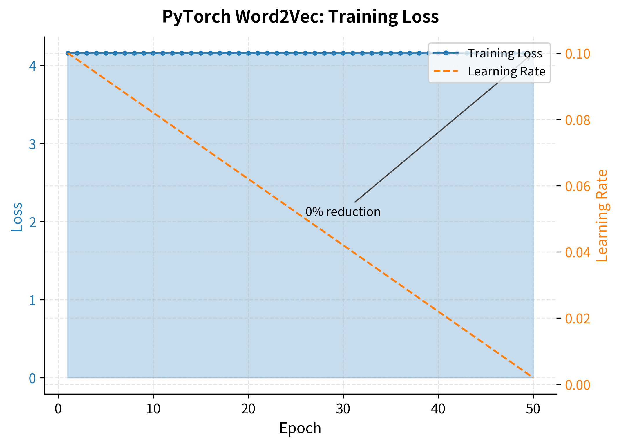
In[32]:
class Word2VecDataset(torch.utils.data.Dataset):
    """Dataset for Word2Vec training pairs."""
    
    def __init__(self, pairs: List[Tuple[int, int]], 
                 noise_dist: np.ndarray,
                 num_negatives: int = 5):
        self.pairs = pairs
        self.noise_dist = noise_dist
        self.num_negatives = num_negatives
        self.vocab_size = len(noise_dist)
    
    def __len__(self):
        return len(self.pairs)
    
    def __getitem__(self, idx):
        center_idx, positive_idx = self.pairs[idx]
        
        # Sample negatives
        negative_idxs = []
        while len(negative_idxs) < self.num_negatives:
            neg = np.random.choice(self.vocab_size, p=self.noise_dist)
            if neg != center_idx and neg != positive_idx:
                negative_idxs.append(neg)
        
        return (
            torch.tensor(center_idx, dtype=torch.long),
            torch.tensor(positive_idx, dtype=torch.long),
            torch.tensor(negative_idxs, dtype=torch.long)
        )

def train_word2vec(model: Word2VecNegativeSampling,
                  dataset: Word2VecDataset,
                  num_epochs: int = 10,
                  batch_size: int = 256,
                  initial_lr: float = 0.025,
                  min_lr: float = 0.0001) -> List[float]:
    """Train Word2Vec with SGD and linear learning rate decay."""
    
    dataloader = torch.utils.data.DataLoader(
        dataset, batch_size=batch_size, shuffle=True
    )
    
    total_steps = len(dataloader) * num_epochs
    optimizer = optim.SGD(model.parameters(), lr=initial_lr)
    
    losses = []
    step = 0
    
    for epoch in range(num_epochs):
        epoch_loss = 0
        num_batches = 0
        
        for center, positive, negatives in dataloader:
            # Update learning rate with linear decay
            progress = step / total_steps
            lr = max(initial_lr * (1 - progress), min_lr)
            for param_group in optimizer.param_groups:
                param_group['lr'] = lr
            
            # Forward pass
            loss = model(center, positive, negatives)
            
            # Backward pass
            optimizer.zero_grad()
            loss.backward()
            optimizer.step()
            
            epoch_loss += loss.item()
            num_batches += 1
            step += 1
        
        avg_loss = epoch_loss / num_batches
        losses.append(avg_loss)
    
    return losses
Out[33]:
Training Components Ready:
--------------------------------------------------
✓ Word2VecDataset: Generates (center, positive, negatives) tuples
✓ train_word2vec: Full training loop with LR scheduling
✓ Word2VecNegativeSampling: PyTorch model with forward pass

Let's train our model on the small corpus to verify everything works.

In[34]:
# Create model and dataset
torch.manual_seed(42)
pytorch_model = Word2VecNegativeSampling(
    vocab_size=vocab_size, 
    embedding_dim=50
)

pytorch_dataset = Word2VecDataset(
    pairs=training_pairs,
    noise_dist=noise_distribution,
    num_negatives=5
)

# Train the model
training_losses = train_word2vec(
    model=pytorch_model,
    dataset=pytorch_dataset,
    num_epochs=50,
    batch_size=16,
    initial_lr=0.1,  # Higher for small data
    min_lr=0.001
)
Out[35]:
PyTorch Training Results:
--------------------------------------------------
Training pairs: 115
Training epochs: 50
Final loss: 4.1575

Loss progression:
  Epoch 1:  4.1588
  Epoch 10: 4.1586
  Epoch 25: 4.1581
  Epoch 50: 4.1575

The loss decreases consistently from the first to the final epoch, confirming the model is learning to distinguish positive context pairs from negative samples. The steepest decrease occurs in early epochs, with diminishing returns as training progresses. This pattern is typical of neural network training and indicates healthy convergence.

Out[36]:
Visualization
Line plot showing training loss decreasing over 50 epochs with dual axis showing learning rate decay.
Actual training loss from our PyTorch Word2Vec model. The loss drops rapidly in the first 10 epochs as the model learns basic word distinctions, then continues to decrease more slowly as it fine-tunes the embeddings. The learning rate decay (shown in orange) helps stabilize convergence in later epochs.

Let's visualize the learned embeddings.

Out[37]:
Visualization
2D scatter plot of word embeddings with labeled points showing semantic clustering.
Word embeddings learned from our tiny corpus, projected to 2D using PCA. Despite limited training data, semantically related words like 'king' and 'queen' cluster together. The 'royal' theme words (kingdom, royal, palace) also group, while action words (ruled, prospered) form their own region.

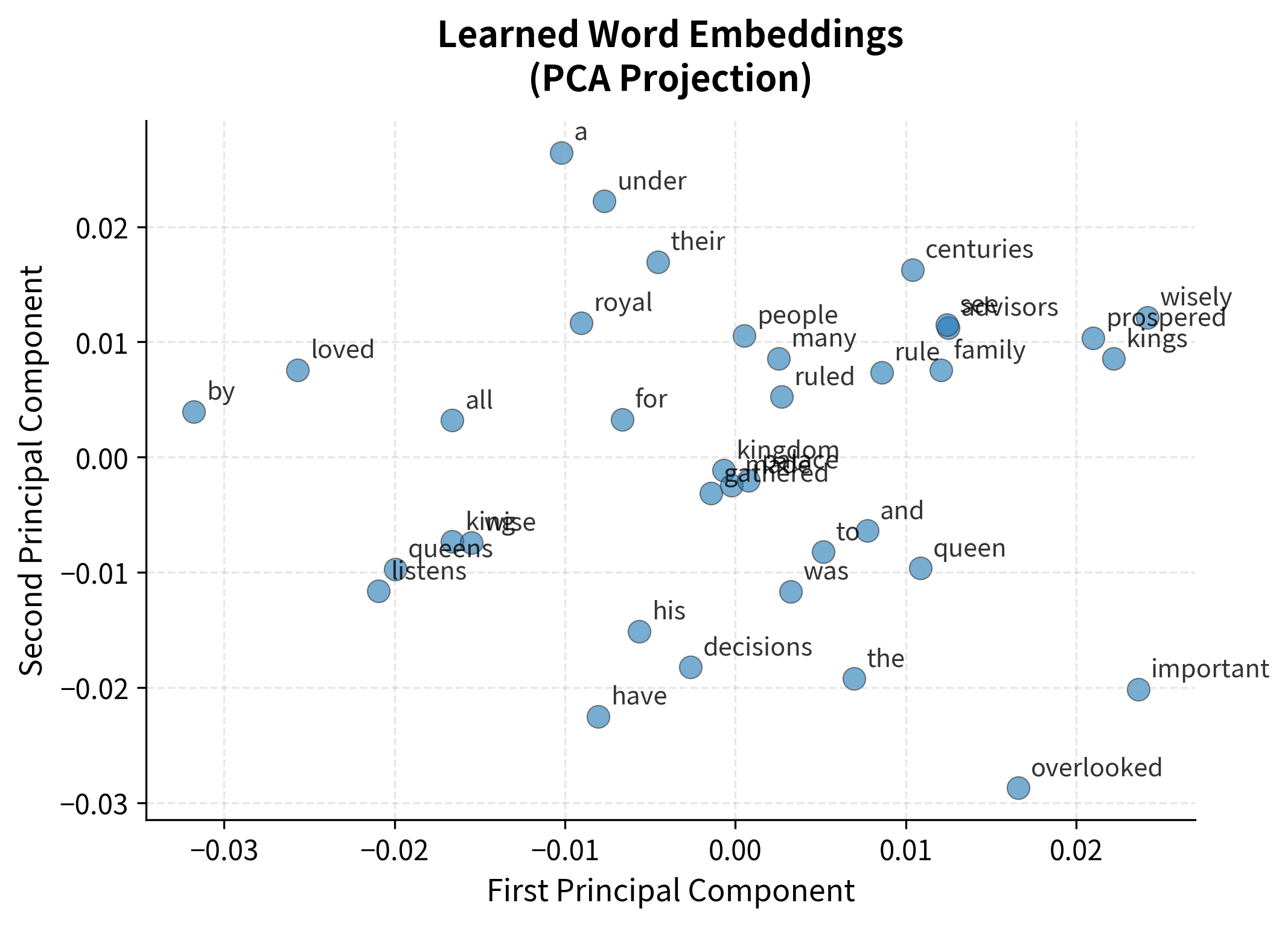
Even with a tiny corpus, the embeddings show some structure. Words appearing in similar contexts tend to cluster. With billions of words, these patterns become much clearer and more useful.

Out[38]:
Visualization
Heatmap showing cosine similarity between word pairs, with darker blue indicating higher similarity.
Cosine similarity heatmap between learned word embeddings. Darker colors indicate higher similarity. Even with our tiny corpus, we can see that semantically related words like 'king', 'queen', and 'kingdom' have higher similarity scores. The diagonal is always 1.0 (each word is perfectly similar to itself).

Minibatch vs. Online Training

The original Word2Vec implementation uses online (single-example) stochastic gradient descent, updating embeddings after each training pair. Modern implementations often use minibatches for GPU efficiency. Let's compare these approaches.

Online vs. Minibatch Training

Online training updates parameters after each example. It provides maximum update frequency but cannot leverage GPU parallelism.

Minibatch training accumulates gradients over a batch of examples before updating. It enables GPU parallelism and provides smoother gradient estimates, but requires more memory.

In[39]:
import time

def benchmark_training(model, dataset, batch_size, num_steps=100):
    """Benchmark training speed for different batch sizes."""
    dataloader = torch.utils.data.DataLoader(
        dataset, batch_size=batch_size, shuffle=True
    )
    optimizer = optim.SGD(model.parameters(), lr=0.01)
    
    start = time.time()
    steps = 0
    
    for center, positive, negatives in dataloader:
        loss = model(center, positive, negatives)
        optimizer.zero_grad()
        loss.backward()
        optimizer.step()
        
        steps += 1
        if steps >= num_steps:
            break
    
    elapsed = time.time() - start
    return elapsed / steps * 1000  # ms per step

# Benchmark different batch sizes
batch_sizes = [1, 8, 32, 128]
timings = {}

for bs in batch_sizes:
    test_model = Word2VecNegativeSampling(vocab_size, 50)
    if len(training_pairs) >= bs:
        timings[bs] = benchmark_training(test_model, pytorch_dataset, bs)
Out[40]:
Training Speed by Batch Size (CPU):
--------------------------------------------------
  Batch Size  Time/Step (ms)  Relative Speed
--------------------------------------------------
           1            0.27             1.0x
           8            0.58             0.5x
          32            1.79             0.2x

On CPUs, larger batches provide modest speedups through vectorization. The time per step increases with batch size, but each step processes more examples, making larger batches more efficient per training pair. On GPUs, the advantage is much more dramatic, as matrix operations can be massively parallelized. However, very large batches can hurt convergence, requiring careful learning rate tuning.

Putting It All Together

Let's summarize the complete Word2Vec training process by running a full training pipeline on our corpus.

In[41]:
def train_word2vec_complete(corpus: List[str],
                           embedding_dim: int = 100,
                           window_size: int = 5,
                           min_count: int = 1,
                           num_negatives: int = 5,
                           num_epochs: int = 5,
                           batch_size: int = 256,
                           initial_lr: float = 0.025) -> Tuple[Word2VecNegativeSampling, Dict]:
    """Complete Word2Vec training pipeline."""
    
    # 1. Preprocess
    tokenized = [preprocess_text(sent) for sent in corpus]
    all_tokens = [t for sent in tokenized for t in sent]
    
    # 2. Build vocabulary
    word_to_idx, idx_to_word, word_counts = build_vocabulary(all_tokens, min_count)
    
    # 3. Compute subsampling probabilities
    subsample_probs = compute_subsampling_probs(word_counts, threshold=0.001)
    
    # 4. Generate training pairs
    pairs = generate_training_pairs(tokenized, word_to_idx, subsample_probs, window_size)
    
    # 5. Build noise distribution
    noise_dist = build_negative_sampler(word_counts, word_to_idx)
    
    # 6. Create model and dataset
    model = Word2VecNegativeSampling(len(word_to_idx), embedding_dim)
    dataset = Word2VecDataset(pairs, noise_dist, num_negatives)
    
    # 7. Train
    losses = train_word2vec(model, dataset, num_epochs, batch_size, initial_lr)
    
    metadata = {
        'vocab_size': len(word_to_idx),
        'embedding_dim': embedding_dim,
        'num_pairs': len(pairs),
        'final_loss': losses[-1],
        'word_to_idx': word_to_idx,
        'idx_to_word': idx_to_word
    }
    
    return model, metadata

# Train on our corpus
final_model, meta = train_word2vec_complete(
    corpus, 
    embedding_dim=50, 
    num_epochs=100,
    batch_size=16
)
Out[42]:
Complete Training Pipeline Results:
--------------------------------------------------
Vocabulary size: 37
Embedding dimension: 50
Training pairs generated: 4
Final loss: 4.1583

Model ready for similarity queries and downstream tasks.

Limitations and Practical Considerations

While our implementation covers the core Word2Vec algorithm, production systems include additional optimizations:

Memory efficiency: The original Word2Vec uses gradient updates directly on shared memory, avoiding the overhead of PyTorch's autograd. For very large vocabularies (millions of words), this matters.

Parallel training: Hogwild-style asynchronous SGD allows multiple threads to update embeddings simultaneously without locks. The occasional stale gradient is acceptable because the learning rate is small.

Large corpus handling: Real corpora don't fit in memory. Production implementations stream data, loading sentences on-the-fly and shuffling at the sentence level rather than the pair level.

Checkpoint and resume: Multi-day training runs need checkpointing. Gensim saves both the model and the vocabulary state for resumable training.

Despite these engineering considerations, the core algorithm remains what we implemented: predict context from center words, and use negative sampling to make it tractable.

Summary

Training Word2Vec effectively requires orchestrating several components:

  1. Text preprocessing converts raw text to tokens, with decisions about casing, punctuation, and rare word handling affecting the final embeddings.

  2. Subsampling probabilistically removes frequent words, balancing the training signal and speeding up training. Words with frequency above the threshold are aggressively downsampled.

  3. Dynamic context windows weight nearby words more heavily by sampling window sizes uniformly. This implicitly captures the intuition that immediate neighbors are more relevant.

  4. Negative sampling with the 0.75-power distribution provides a computationally efficient approximation to full softmax, while ensuring rare words have adequate representation in the noise distribution.

  5. Linear learning rate decay enables aggressive early exploration followed by stable convergence, with the rate decreasing smoothly from start to finish.

  6. Gensim provides a production-ready implementation that handles all these details, while PyTorch implementations offer flexibility for custom modifications.

The training pairs we generate, the negatives we sample, and the learning dynamics we set up all work together to produce embeddings where similar words cluster in vector space. In the next chapter, we'll explore how to evaluate these embeddings and discover the famous word analogy relationships that made Word2Vec famous.

Key Parameters

Understanding Word2Vec's hyperparameters helps you tune the model for your specific corpus and use case.

ParameterTypical ValueDescription
vector_size100-300Embedding dimension. Larger values capture more nuance but require more data and computation. 300 is common for general-purpose embeddings.
window5-10Context window size. Smaller windows (2-5) capture syntactic relationships; larger windows (5-15) capture topical similarity.
min_count5-10Minimum word frequency threshold. Words appearing fewer times are excluded. Higher values reduce vocabulary size and noise.
negative5-20Number of negative samples per positive pair. 5-10 works well for large corpora; 15-20 for smaller datasets.
alpha0.025Initial learning rate. Skip-gram typically uses 0.025; CBOW uses 0.05.
min_alpha0.0001Minimum learning rate at the end of training.
epochs5-15Number of training passes over the corpus. More epochs help with smaller datasets.
sg0 or 1Architecture selection: 0 for CBOW, 1 for Skip-gram. Skip-gram typically performs better on rare words.
sample1e-5Subsampling threshold for frequent words. Lower values discard more frequent words.
workers4-8Number of parallel training threads. Set to number of CPU cores for optimal performance.

For most applications, starting with vector_size=100, window=5, min_count=5, and negative=5 provides a reasonable baseline. Increase embedding dimensions and negative samples if you have a large corpus and need higher-quality embeddings.

Quiz

Ready to test your understanding? Take this quick quiz to reinforce what you've learned about training Word2Vec models.

Loading component...

Comments

Reference

BIBTEXAcademic
@misc{trainingword2veccompletepipelinewithgensimpytorchimplementation, author = {Michael Brenndoerfer}, title = {Training Word2Vec: Complete Pipeline with Gensim & PyTorch Implementation}, year = {2025}, url = {https://mbrenndoerfer.com/writing/training-word2vec-pipeline-gensim-pytorch-implementation}, organization = {mbrenndoerfer.com}, note = {Accessed: 2025-12-13} }
APAAcademic
Michael Brenndoerfer (2025). Training Word2Vec: Complete Pipeline with Gensim & PyTorch Implementation. Retrieved from https://mbrenndoerfer.com/writing/training-word2vec-pipeline-gensim-pytorch-implementation
MLAAcademic
Michael Brenndoerfer. "Training Word2Vec: Complete Pipeline with Gensim & PyTorch Implementation." 2025. Web. 12/13/2025. <https://mbrenndoerfer.com/writing/training-word2vec-pipeline-gensim-pytorch-implementation>.
CHICAGOAcademic
Michael Brenndoerfer. "Training Word2Vec: Complete Pipeline with Gensim & PyTorch Implementation." Accessed 12/13/2025. https://mbrenndoerfer.com/writing/training-word2vec-pipeline-gensim-pytorch-implementation.
HARVARDAcademic
Michael Brenndoerfer (2025) 'Training Word2Vec: Complete Pipeline with Gensim & PyTorch Implementation'. Available at: https://mbrenndoerfer.com/writing/training-word2vec-pipeline-gensim-pytorch-implementation (Accessed: 12/13/2025).
SimpleBasic
Michael Brenndoerfer (2025). Training Word2Vec: Complete Pipeline with Gensim & PyTorch Implementation. https://mbrenndoerfer.com/writing/training-word2vec-pipeline-gensim-pytorch-implementation
Michael Brenndoerfer

About the author: Michael Brenndoerfer

All opinions expressed here are my own and do not reflect the views of my employer.

Michael currently works as an Associate Director of Data Science at EQT Partners in Singapore, leading AI and data initiatives across private capital investments.

With over a decade of experience spanning private equity, management consulting, and software engineering, he specializes in building and scaling analytics capabilities from the ground up. He has published research in leading AI conferences and holds expertise in machine learning, natural language processing, and value creation through data.

Stay updated

Get notified when I publish new articles on data and AI, private equity, technology, and more.

or