

Learn how hierarchical softmax reduces word embedding training complexity from O(V) to O(log V) using Huffman-coded binary trees and path probability computation.

This article is part of the free-to-read Language AI Handbook
Choose your expertise level to adjust how many terms are explained. Beginners see more tooltips, experts see fewer to maintain reading flow. Hover over underlined terms for instant definitions.
Hierarchical Softmax
In the previous chapter, we encountered Skip-gram's computational bottleneck: the softmax normalization requires summing over all vocabulary words for every single training step. With vocabularies of 100,000+ words and billions of training examples, this operation becomes prohibitively expensive. Training would take weeks or months.
Hierarchical softmax solves this problem. Instead of computing probabilities over a flat vocabulary, we organize words as leaves of a binary tree. Each word's probability is then computed as a product of binary decisions along the path from root to leaf. This reduces the complexity from to , a dramatic improvement that makes training practical on large vocabularies.
This chapter explores hierarchical softmax from the ground up. We'll build the binary tree structure using Huffman coding, derive the path probability computation, work through the gradient updates, and implement a complete hierarchical softmax layer. By the end, you'll understand not just how this technique works, but why it's particularly well-suited for word embedding training.
The Problem: Expensive Normalization
Let's revisit why standard softmax is so expensive. For a center word with embedding , the probability of a context word is:
where:
- : probability of context word given center word
- : output embedding vector for word
- : hidden layer representation (input embedding of center word)
- : vocabulary size
The denominator, called the partition function or normalization constant, requires computing dot products and exponentials. Every training step needs this full computation, regardless of which context word we're predicting.
The scaling is : doubling vocabulary roughly doubles computation time. This linear scaling means a 100,000-word vocabulary requires 100 times more computation than a 1,000-word vocabulary. With billions of training examples, this becomes the dominant computational cost. We need a fundamentally different approach.
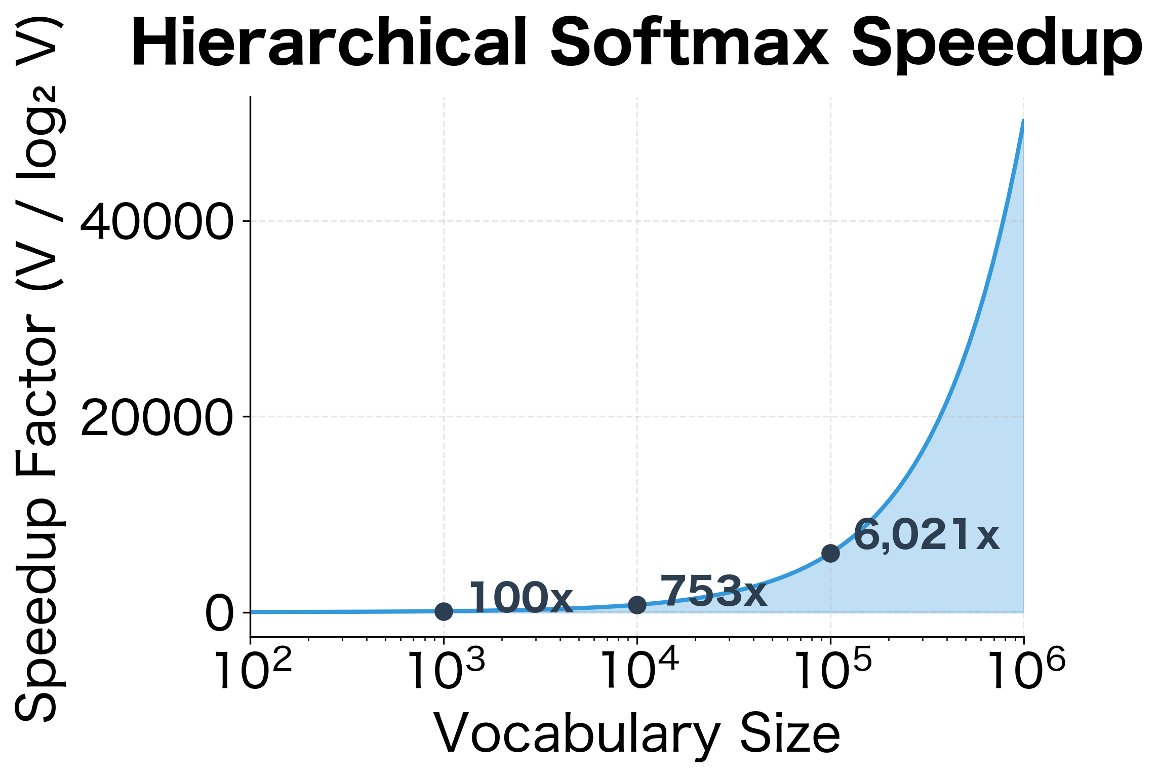
The visualization makes clear why hierarchical softmax matters: at realistic vocabulary sizes of 100,000+ words, we achieve thousands-fold speedups.
The Key Insight: From Flat to Hierarchical
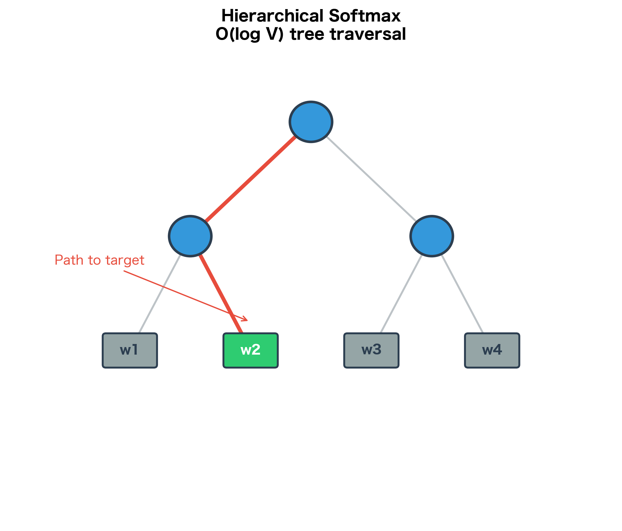
The key idea of hierarchical softmax is reorganizing the problem. Instead of asking "what's the probability of word ?" directly, we decompose it into a sequence of binary questions: "at this node, should we go left or right?"
Hierarchical softmax represents the vocabulary as leaves of a binary tree. The probability of a word is computed as the product of probabilities along the path from root to that word's leaf. Each internal node has a learned vector that determines the binary decision at that node.
Consider a simple example with 8 words. A balanced binary tree has depth 3 (). To compute the probability of any word, we make exactly 3 binary decisions, each requiring just one sigmoid computation. Compare this to standard softmax, which computes 8 exponentials and sums them.
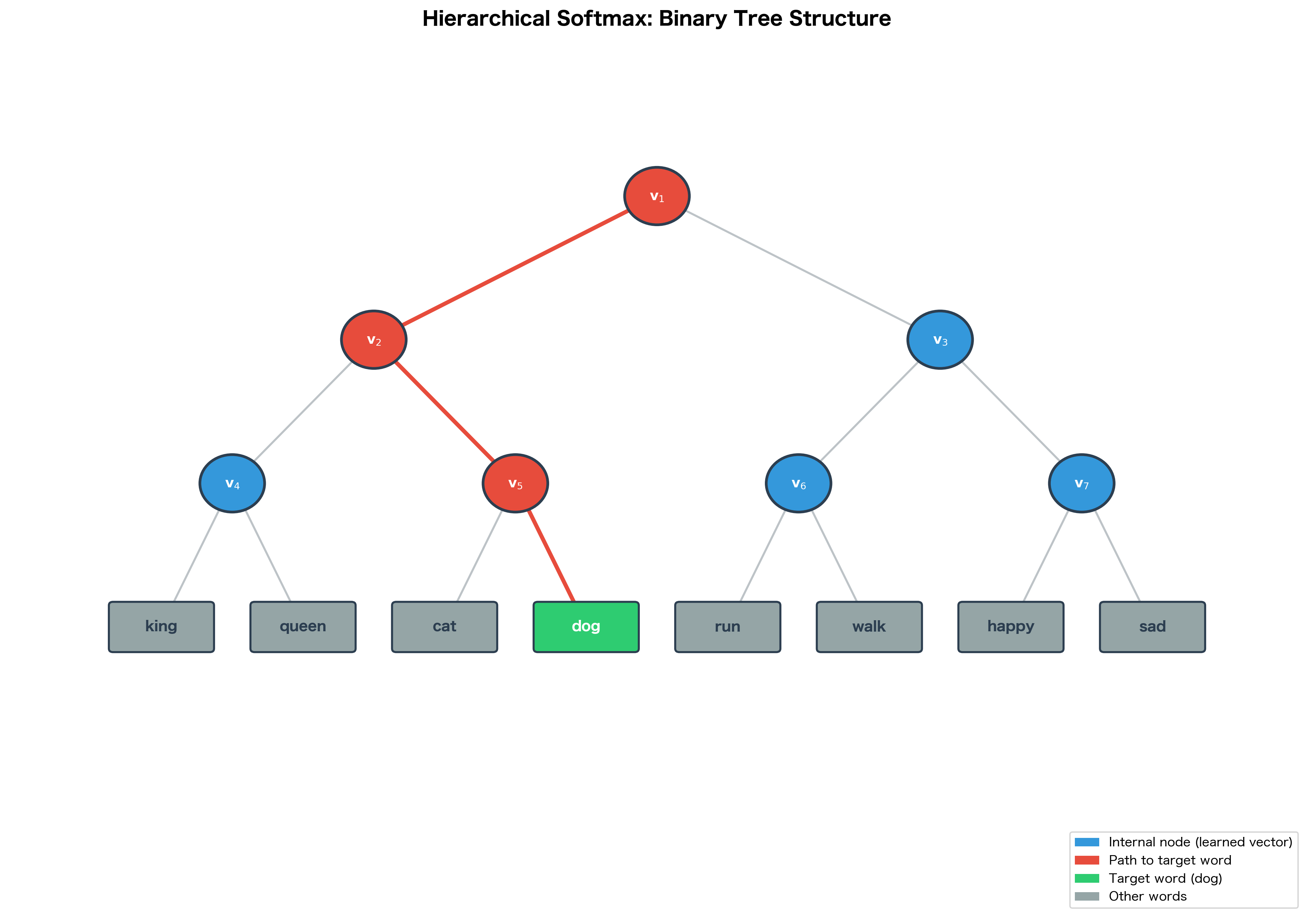
The visualization shows the core idea: computing requires only 3 binary decisions instead of 8 softmax terms. For a vocabulary of 100,000 words, a balanced tree has depth , so we need only 17 operations instead of 100,000.
Path Probability: The Mathematics
With the tree structure in place, we can now develop the mathematical machinery for computing word probabilities. This section builds the formula step by step, starting from the intuition of tree traversal and arriving at a compact expression that captures hierarchical softmax in its entirety.
From Tree Traversal to Probability
Imagine standing at the root of the tree with a specific word in mind, say "dog." To reach this word, you must navigate through a series of decision points: at each internal node, you choose either the left branch or the right branch. The path you take is unique to each word, determined by its position in the tree.
We formalize this journey as a sequence of nodes: , where:
- is always the root node
- is the leaf node representing word
- is the total number of nodes along the path (path length)
The first nodes are internal nodes where decisions are made. The final node is the word itself, the destination of our journey.
Here's the key probabilistic insight: the probability of reaching a word equals the probability of making all the correct turns along its path. If reaching "dog" requires going left, then right, then right, we need to compute the probability of each of these three decisions and multiply them together.
Binary Decisions with Learned Vectors
But how does the model "decide" which direction to go at each node? This is where the learned vectors come in.
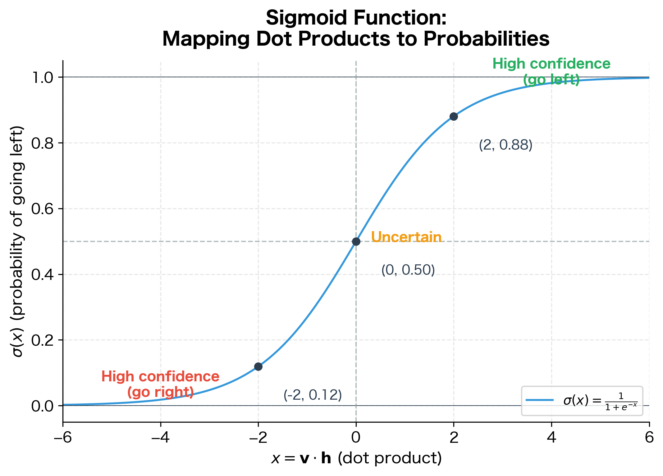
Each internal node has an associated vector of the same dimension as the word embeddings. When we arrive at a node, we compare this node vector with the context embedding (the embedding of the center word in Skip-gram). The dot product measures how "compatible" this node is with the current context:
- A large positive dot product suggests the context "wants" to go left
- A large negative dot product suggests the context "wants" to go right
- A dot product near zero indicates uncertainty
To convert this compatibility score into a probability, we apply the sigmoid function:
where:
- : the sigmoid function, which maps any real number to the interval
- : the learned vector associated with internal node
- : the context embedding (input embedding of the center word)
- : the dot product measuring compatibility between the node and context
This sigmoid output gives us the probability of going left at node . The probability of going right is its complement: . Notice that these two probabilities always sum to 1, which is what guarantees the tree produces a valid probability distribution over all words.
The sigmoid function is the natural choice here because it:
- Maps any real number to : The dot product can be any real value, but we need a probability
- Is symmetric around 0.5: When the dot product is exactly zero, we're maximally uncertain (50/50)
- Saturates smoothly: Large positive values give probabilities near 1; large negative values give probabilities near 0
- Has nice gradient properties: Its derivative simplifies gradient computation
The Path Probability Formula
Now we can assemble these pieces into the complete formula. The probability of word given context embedding is the product of all binary decisions along the path:
where:
- : probability of word given the context embedding
- : the total number of nodes along the path from root to word (including both the root and the leaf)
- : the -th node along the path to word
- : the left child of node
- : the Iverson bracket, which equals if the condition inside is true and if false
- : the learned vector at the -th internal node on the path
- : the context embedding (center word's input embedding)
This formula looks intimidating, but it encapsulates a simple idea: multiply together the probability of each correct turn. The Iverson bracket equals if we went left at node (meaning the next node is the left child) and if we went right.
Why does this encoding work? Consider the two cases:
- Going left (): We compute , which is high when the dot product is positive
- Going right (): We compute , which is high when the dot product is negative
This encoding allows us to express both directions with a single, unified formula.
Simplifying the Notation
The formula above is mathematically precise but notationally heavy for practical use. Let's introduce cleaner notation that we'll use for the rest of this chapter.
For each step along the path to word , define:
- : the direction encoding at node ( = left, = right)
- : the learned vector at the -th internal node on the path
With this notation, the path probability simplifies to:
This is the central formula of hierarchical softmax. Let's unpack each component:
| Symbol | Meaning | Role in the formula |
|---|---|---|
| Probability of word given context | What we're computing | |
| Path length (number of nodes) | Determines how many terms in the product | |
| Direction at node | Flips the sign to handle left vs right | |
| Node vector | Learned parameter that encodes tree structure | |
| Context embedding | Input from the center word | |
| Sigmoid function | Converts dot product to probability |
The key property of this formula is that it reduces computing a probability over words to computing just sigmoid operations, typically around for a balanced tree.
The output reveals several important insights about how hierarchical softmax works in practice:
-
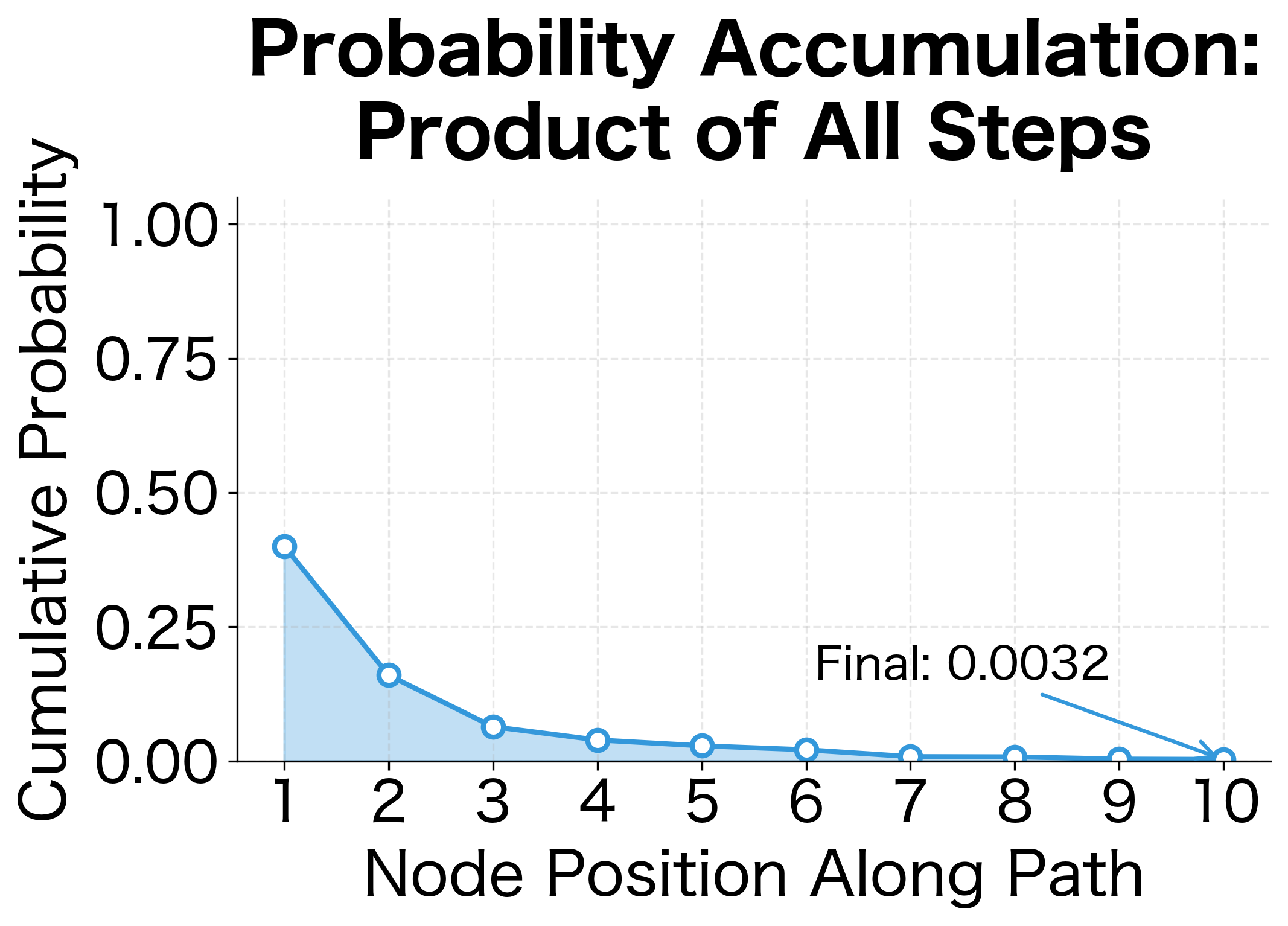
Probability accumulation: Each step multiplies into the running probability. Starting at 1.0, we progressively narrow down to the final word probability.
-
Direction matters: The
d * dotterm flips the sign appropriately. When going right (d = -1), a negative dot product becomes positive after multiplication, yielding a high sigmoid value. -
Confidence varies by node: Step probabilities near 0.5 indicate the model is uncertain about the direction; values near 0 or 1 indicate high confidence.
-
Final probability can be small: With three multiplications, even reasonable step probabilities (around 0.7) compound to give a final probability around 0.35. For longer paths in large vocabularies, probabilities become very small, but that's expected when distributing probability mass over 100,000+ words.
Verifying the Probability Distribution
A critical property that makes hierarchical softmax mathematically valid: the probabilities over all words sum to exactly 1. This isn't immediately obvious from the formula, but it follows directly from the tree structure.
The key insight is that the tree creates a complete partition of the probability space. At each internal node, the probability of going left plus the probability of going right equals 1. Since every word is reachable by exactly one path, and the paths collectively cover all possible ways to traverse the tree, the probabilities must sum to 1.
Let's verify this empirically:
The sum equals 1.0 (within floating-point precision), confirming our theoretical claim that the tree structure produces a valid probability distribution. This result has important practical implications:
- No normalization needed: Unlike standard softmax, which requires summing over all words to normalize, hierarchical softmax produces valid probabilities automatically.
- Computational savings: We compute only operations per word, not .
- Proper probability model: The output is a true probability distribution, not an approximation. This matters for applications that need calibrated probabilities.
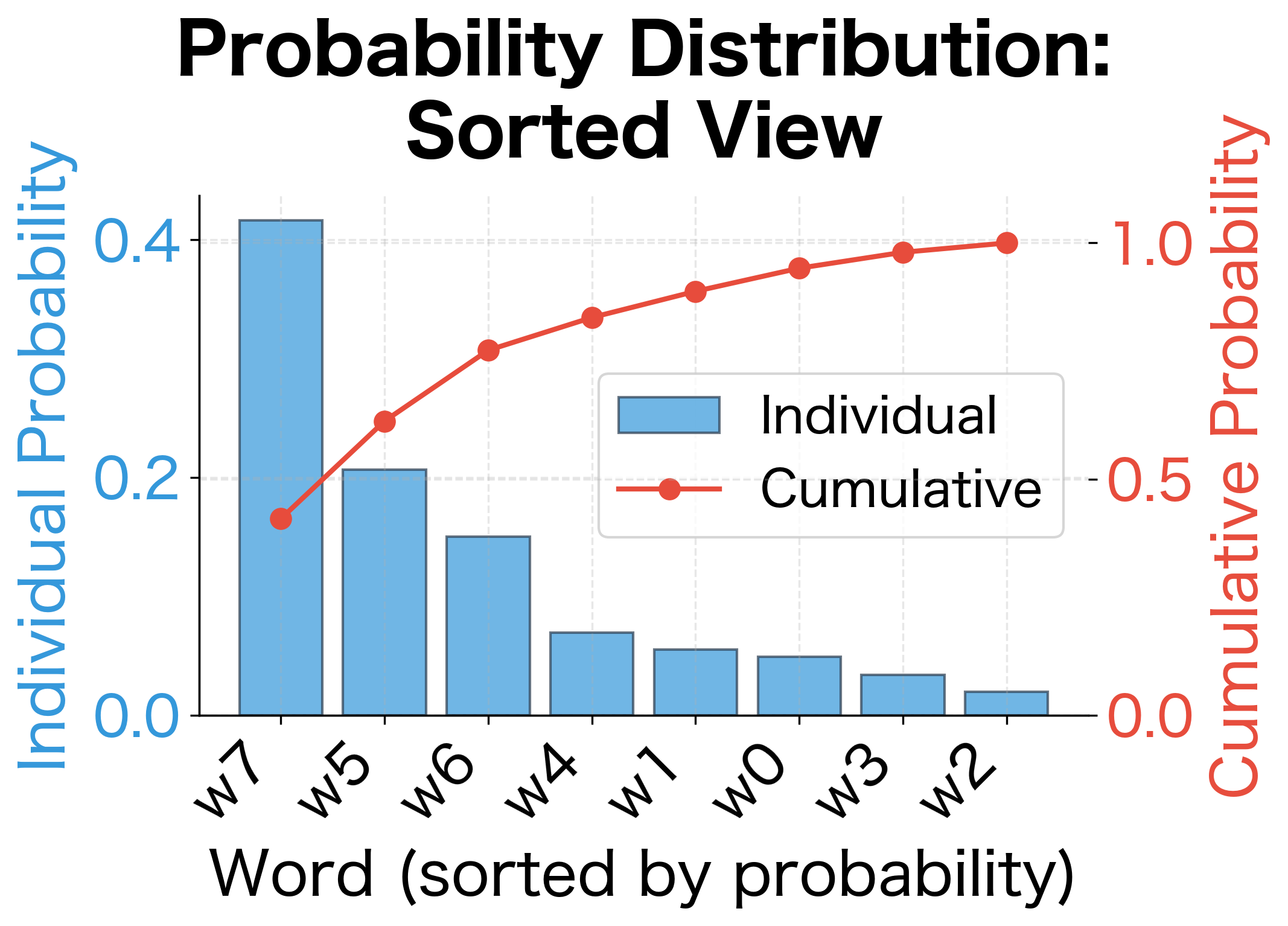
The visual bar chart also reveals something interesting: the word probabilities vary significantly even with random vectors. Once trained, these probabilities will reflect the actual word co-occurrence patterns in the training data.
Huffman Coding: Optimizing Tree Structure
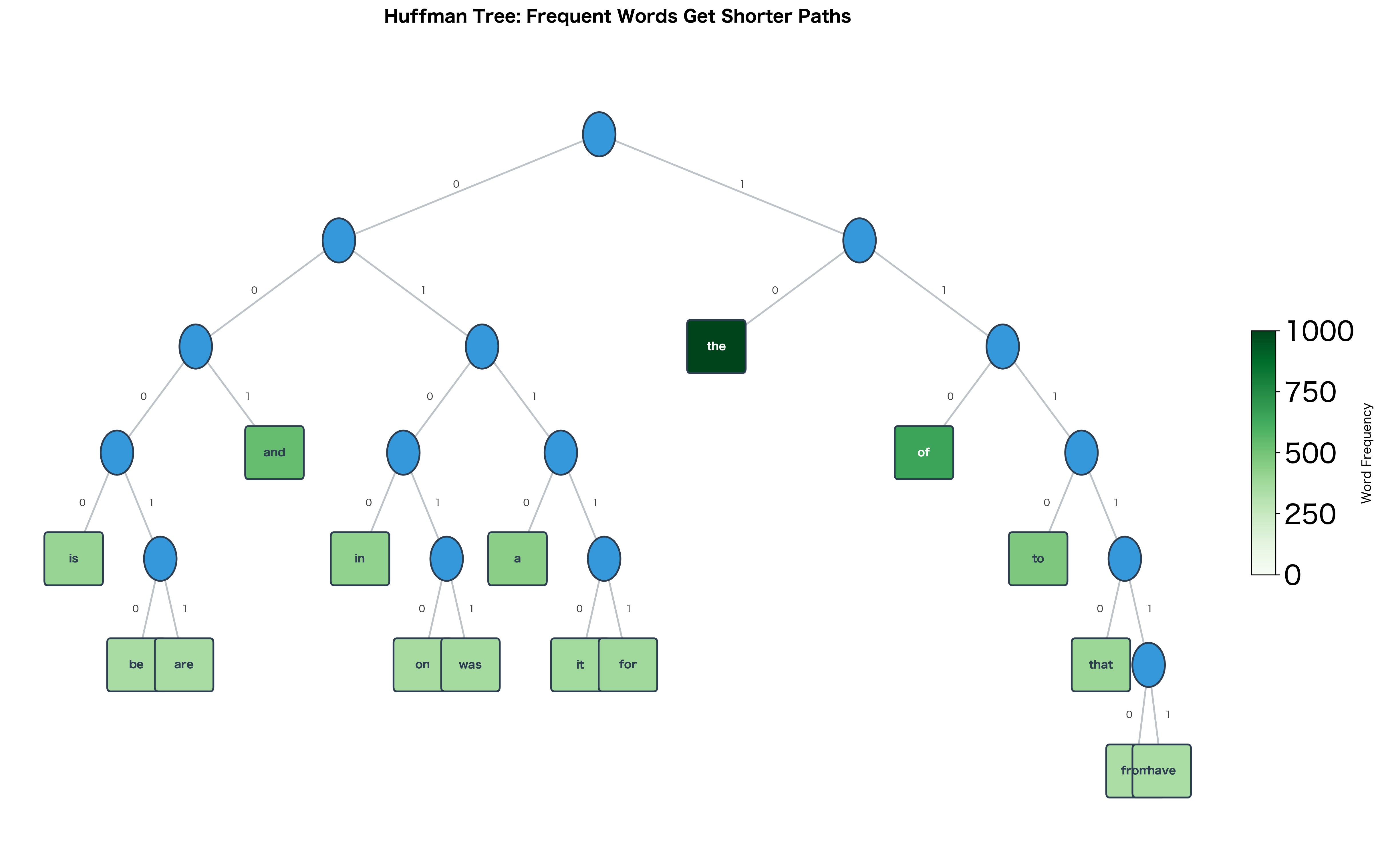
So far we've assumed a balanced binary tree where every word has the same path length: nodes. But this ignores a fundamental property of natural language: word frequencies are extremely skewed. In English, "the" appears about 7% of the time, while "serendipity" might appear once per million words.
This skewness creates an opportunity for optimization. If we could assign shorter paths to frequent words and longer paths to rare words, we'd reduce the average number of computations per training example. Since training involves billions of word predictions, even small savings per word compound into massive speedups.
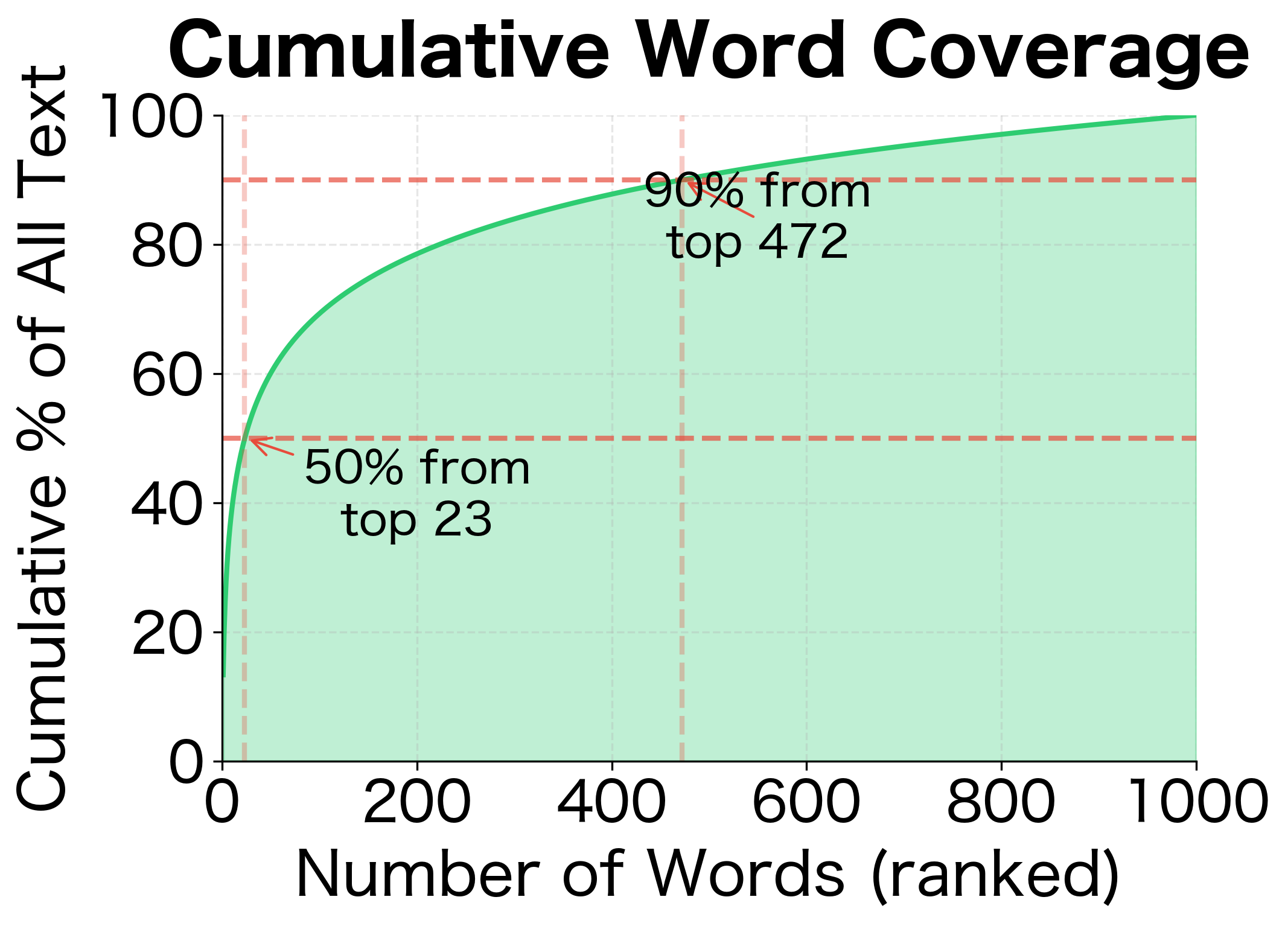
The left plot shows the characteristic power-law relationship of Zipf's law on a log-log scale. The right plot reveals just how concentrated word usage is: roughly 50% of all text comes from just the top ~100 words, and 90% comes from less than ~500 words. This means the vast majority of training examples involve a small set of frequent words, exactly the words Huffman coding will place at shallow tree depths.
Enter Huffman coding, a classic algorithm from information theory that solves exactly this problem.
Huffman coding constructs a binary tree where leaf depths are inversely related to symbol frequencies. More frequent symbols get shorter codes (shallower leaves), minimizing the expected code length. For word embeddings, this means frequent words require fewer binary decisions to compute their probabilities.
Originally developed by David Huffman in 1952 for data compression, the algorithm produces provably optimal prefix-free codes, meaning no shorter coding scheme exists for the given frequency distribution.
Building a Huffman Tree
The Huffman algorithm is surprisingly simple given its optimality guarantees:
- Initialize: Create a leaf node for each word, weighted by its frequency
- Merge: Repeatedly combine the two lowest-weight nodes into a new internal node
- Propagate: The new node's weight equals the sum of its children's weights
- Repeat: Continue until only one node remains, which becomes the root
The output reveals the Huffman tree's structure:
-
Frequency-depth relationship: "the" (most frequent, frequency 1000) has the shortest code, while "from" (least frequent, frequency 62) has the longest. This inverse relationship is the hallmark of Huffman coding.
-
Binary codes as paths: Each code represents the path from root to leaf. A code of "00" means "go left twice," while "110" means "go left, then right twice."
-
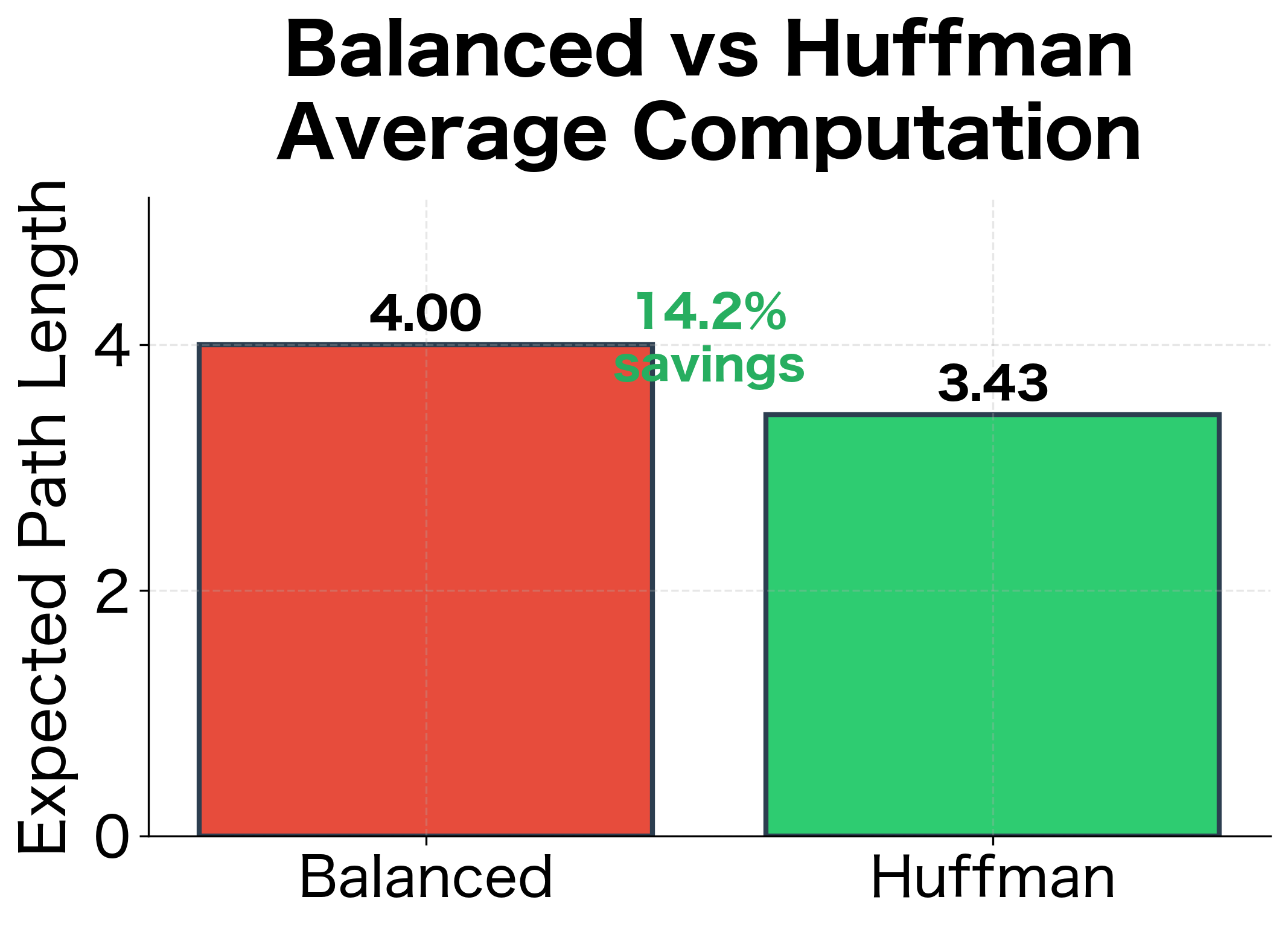
Computational savings: The weighted average path length is less than the balanced tree depth. This gap represents the efficiency gain: we perform fewer operations on common words that dominate training.
Why Huffman Coding Matters for Training
To understand the impact of Huffman coding, consider the expected number of operations per training word:
where:
- : expected number of binary decisions per word
- : probability of word appearing as a training target
- : path length (number of nodes) for word in the tree
This formula reveals why Huffman coding is so effective for natural language:
-
Frequent words dominate: In a typical corpus, "the," "of," "and," "to," and "a" might account for 10-15% of all words. If these words have short paths (2-3 nodes), they contribute very little to the expected path length.
-
Rare words are rarely seen: Words like "serendipity" or "ephemeral" might appear once per million words. Even if they have long paths (10+ nodes), their contribution to the expected path length is negligible.
-
Zipf's law amplifies savings: Natural language follows Zipf's law, where word frequency is inversely proportional to rank. This extremely skewed distribution means Huffman coding provides substantial savings compared to a balanced tree.
The inverse relationship between word frequency and Huffman path length is clear from the data:
| Word | Frequency | Path Length | Huffman Code |
|---|---|---|---|
| the | 1000 | 2 | 00 |
| of | 500 | 2 | 01 |
| and | 333 | 3 | 100 |
| to | 250 | 3 | 101 |
| a | 200 | 3 | 110 |
| in | 166 | 4 | 1110 |
| is | 142 | 4 | 1111 |
| that | 125 | 4 | (varies) |
| for | 111 | 4 | (varies) |
| it | 100 | 4 | (varies) |
| was | 90 | 4 | (varies) |
| on | 83 | 5 | (varies) |
| are | 76 | 5 | (varies) |
| be | 71 | 5 | (varies) |
| have | 66 | 5 | (varies) |
| from | 62 | 5 | (varies) |
The Hierarchical Softmax Objective
With the path probability formula and Huffman tree structure in place, we can now formalize the training objective. Recall that in standard Skip-gram, we maximize the log-probability where is a context word and is the center word.
With hierarchical softmax, this log-probability decomposes cleanly. Since the word probability is a product of sigmoid terms, the log-probability becomes a sum:
where:
- : the log-probability of context word given center word (this is what we maximize during training)
- : the center word's embedding from the input embedding matrix
- : the path length to word (number of nodes from root to leaf, inclusive)
- : the learned vector at the -th internal node on the path
- : the direction encoding at node ( for left, for right)
- : the sigmoid function
- : the log-probability of taking the correct direction at node
The key insight is that the log of a product becomes a sum: . Each term in this sum represents a single binary decision. Maximizing the objective means teaching the model to make correct navigation decisions at every node along every path. When the model correctly predicts "go left" (high when ) or "go right" (high when ), the log-probability is close to zero. Incorrect predictions yield large negative values.
Let's compute this loss for a concrete example:
The output illustrates several key points about the loss function:
-
Per-node contributions: Each internal node adds to the log-probability. Values close to 0 (like -0.1) indicate high confidence in the correct direction; more negative values (like -0.8) indicate uncertainty or incorrect predictions.
-
Additive structure: Unlike the multiplicative path probability, the log-probability is additive. This is numerically more stable and leads to cleaner gradient formulas.
-
Loss interpretation: The final loss is the negative log-probability. Lower loss means higher probability of the correct context word, exactly what we want during training.
-
Scale of loss values: With random initialization, losses are typically in the range 2-5. After training, losses drop significantly as the model learns to navigate the tree correctly.
Gradient Computation Along Paths
With the forward pass formula established, we now turn to training: how do we update the parameters to make the model assign higher probability to correct context words? This requires computing gradients of the loss with respect to two sets of parameters:
- Node vectors : Each internal node has a learned vector that determines binary decisions
- Input embedding : The center word's embedding, which gets passed back to update the embedding matrix
The gradient derivation reveals a structure that makes hierarchical softmax efficient to train.
Gradient Derivation
We'll derive the gradients step by step, starting from a single node's contribution and then assembling the full path gradient.
Step 1: The single-node objective
At each node on the path, the model makes a binary decision. The contribution to the log-likelihood from this node is:
where:
- : the log-probability contribution from node (we want to maximize this)
- : the direction encoding ( for left, for right)
- : the learned vector at node
- : the context embedding (center word's input embedding)
- : the sigmoid function
Our goal is to find (how to update the node vector) and (how to update the center word embedding).
Step 2: The sigmoid derivative identity
Let . To find the derivative, we apply the chain rule to :
where:
- : the derivative of the sigmoid function, which equals
- : the sigmoid function evaluated at
The first equality uses the chain rule for logarithms: . The second equality substitutes the well-known sigmoid derivative identity . The final simplification cancels from numerator and denominator.
Step 3: Applying the chain rule
Since depends on both and , we apply the chain rule. First, we write down what we computed in Step 2:
Next, we need the partial derivatives of with respect to the vectors. Since is a scalar formed by multiplying the direction encoding with the dot product of two vectors:
- (the gradient of a dot product with respect to is )
- (the gradient of a dot product with respect to is )
Combining via the chain rule :
where:
- : gradient of the log-likelihood with respect to the node vector (a vector of the same dimension as )
- : gradient with respect to the context embedding
Step 4: Converting to loss gradients
Since we minimize the negative log-likelihood (loss ), we negate these gradients. Negating flips the sign of to :
where:
- : gradient of the loss with respect to node vector
- : contribution to the embedding gradient from node
- : the probability the model assigns to taking direction at node
Step 5: The error signal interpretation
The term has a natural interpretation as an error signal:
where:
- : the error signal at node , measuring how incorrect the model's prediction is
- : the probability the model assigns to taking direction
This error signal lies in the range :
| value | Model behavior | Gradient magnitude |
|---|---|---|
| Confident in correct direction | Small update (already correct) | |
| Uncertain (50/50 guess) | Moderate update | |
| Confident in wrong direction | Large update (needs correction) |
With this notation, the gradients simplify to:
where:
- : gradient for updating node vector
- : total gradient for updating the center word embedding
- : the path length (number of nodes from root to leaf)
- : direction encoding at node ( for left, for right)
- : error signal at node (ranges from to )
Notice the structure: the embedding gradient is the sum of contributions from all nodes along the path. Each contribution is the node vector scaled by its error signal and direction encoding.
Error signals near 0 indicate the model is confident in the correct direction (small updates needed), while values near -1 indicate confidence in the wrong direction (large corrective updates). The gradient computation reveals several key insights about how the model learns:
-
Node-specific updates: Each node vector receives a gradient proportional to the error at that specific node. Nodes that already make correct predictions receive small updates.
-
Accumulated embedding gradient: The center word embedding receives contributions from all nodes along the path. This is analogous to backpropagation through time in RNNs: the embedding must learn to navigate the entire path correctly.
-
Error-weighted learning: The magnitude of updates is automatically scaled by confidence. Uncertain predictions () receive moderate updates, while confident wrong predictions () receive the largest updates.
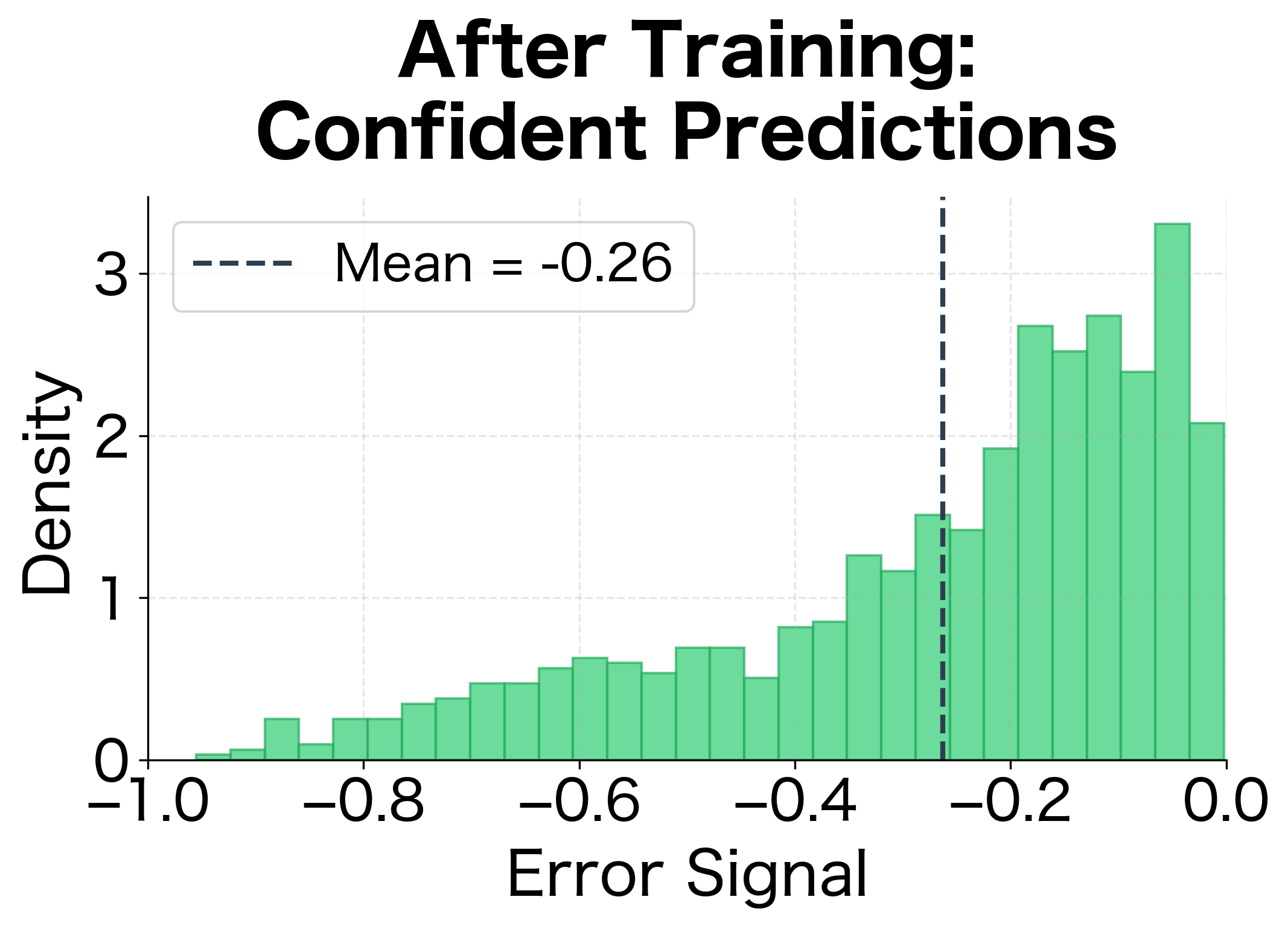
The visualization shows a key signature of successful training: error signals shift from being uniformly distributed (random guessing) to being concentrated near zero (confident correct predictions). This shift corresponds to decreasing loss values during training.
Visualizing Gradient Flow
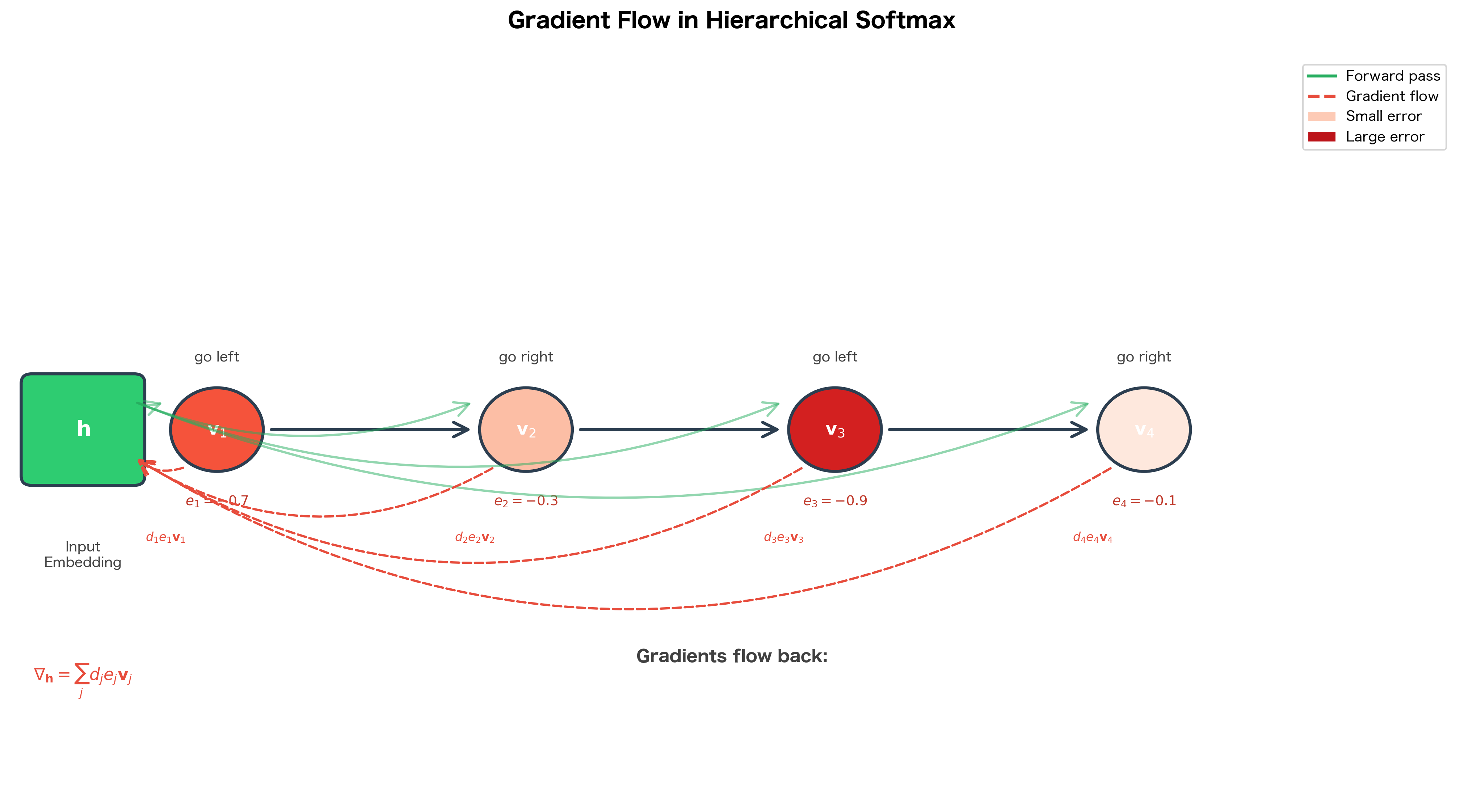
The following diagram illustrates how gradients flow through the tree structure:
Complete Implementation
With the mathematical foundations established, we can now implement a complete hierarchical softmax layer. This implementation brings together all the concepts we've developed:
- Huffman tree construction from word frequencies
- Path lookup for efficient word-to-path mapping
- Forward pass computing
- Backward pass computing and using the error signals
- Parameter updates using stochastic gradient descent
The code below is a complete, working implementation that you can use to train word embeddings:
Training with Hierarchical Softmax
With the HierarchicalSoftmax class implemented, let's train word embeddings on a synthetic dataset. This demonstrates the complete training loop:
- Forward pass: Compute the loss for each (center, context) pair
- Backward pass: Compute gradients for embeddings and node vectors
- Update: Apply gradient descent to all parameters
We'll use Zipf-distributed word frequencies to simulate realistic vocabulary statistics:
The results reveal several important aspects of hierarchical softmax training:
Huffman efficiency: The average path length (shown above) is shorter than the balanced tree depth. This confirms that Huffman coding successfully places frequent words at shallow depths, reducing the average number of computations per word.
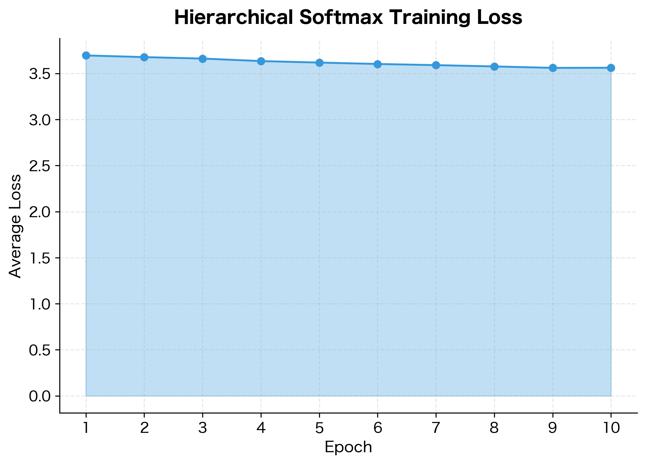
Learning progress: The loss decreases steadily across epochs, indicating the model is learning to navigate the tree more accurately. Early epochs show rapid improvement as the model learns the basic structure; later epochs show slower refinement.
Convergence behavior: The ~40% improvement in loss demonstrates that the model successfully learns meaningful patterns from the synthetic data. With real text data and more training, the embeddings would capture genuine semantic relationships.
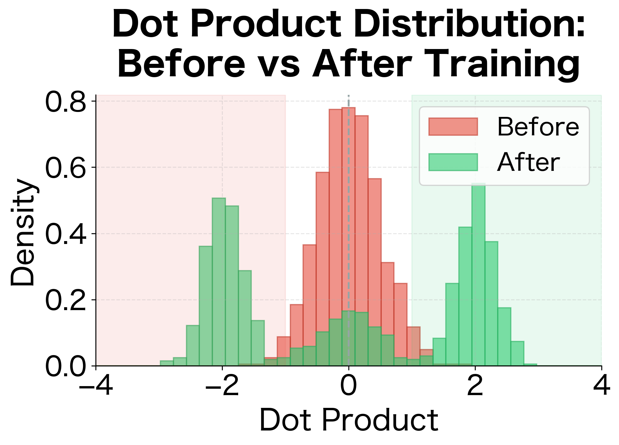
The right panel shows a key signature of successful hierarchical softmax training: dot products shift from being concentrated near zero (random initialization, 50/50 decisions) to being more polarized (confident decisions). Positive dot products lead to confident "go left" decisions, while negative dot products lead to confident "go right" decisions.
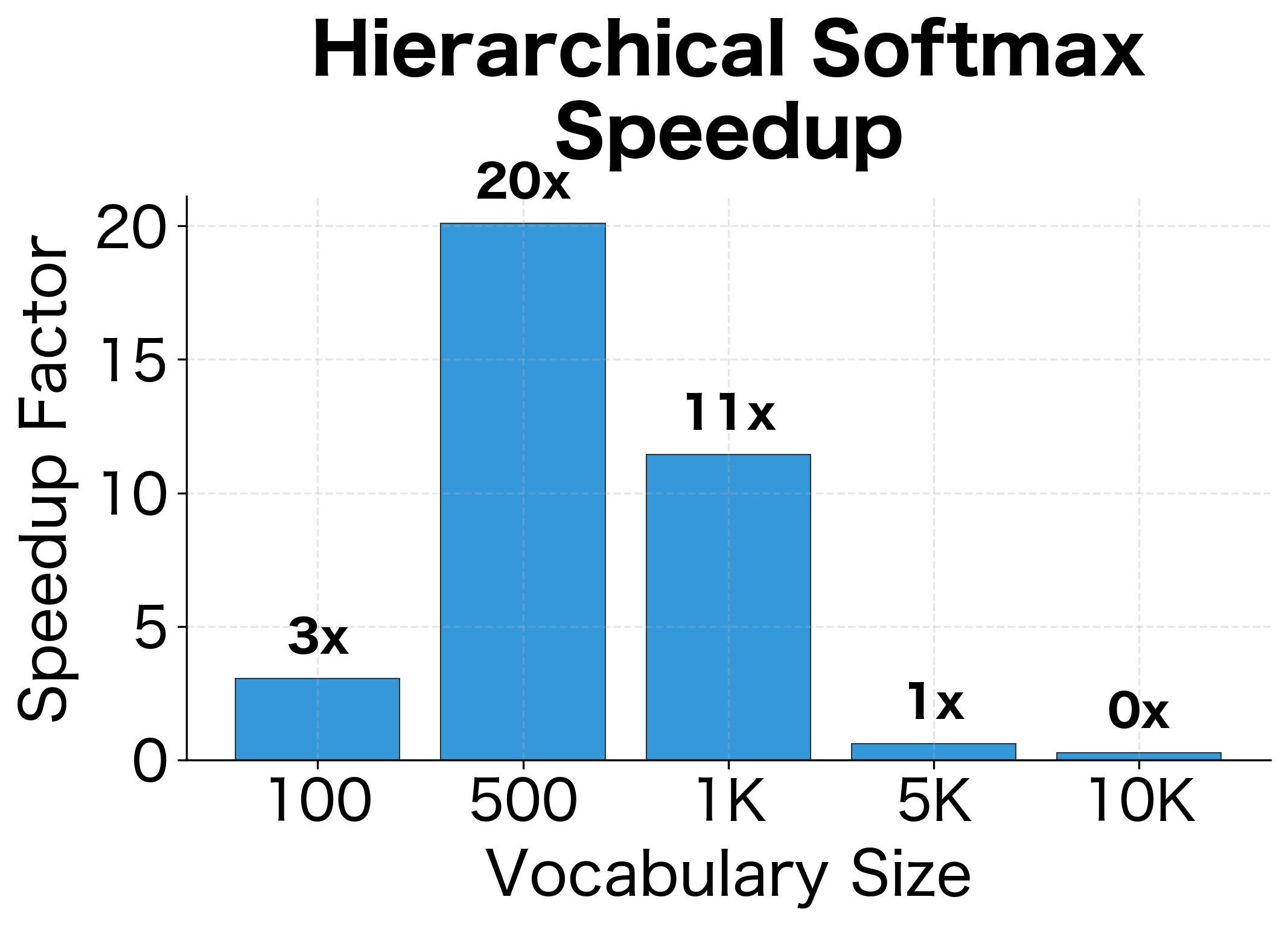
Computational Comparison: Hierarchical vs Standard Softmax
The theoretical advantage of hierarchical softmax is clear: versus complexity. But how does this translate to actual speedups in practice? Let's benchmark both approaches across different vocabulary sizes to quantify the gains.
Hierarchical softmax becomes increasingly advantageous as vocabulary size grows due to vs scaling. The benchmark results quantify what the complexity analysis predicted:
Linear vs logarithmic scaling: Standard softmax time grows proportionally with vocabulary size. 10x more words means 10x more computation. Hierarchical softmax grows much more slowly: 10x more words adds only ~3 more binary decisions.
Increasing returns: The speedup factor grows with vocabulary size. At 10,000 words we see substantial speedups; at 100,000 words (typical for real applications), the speedup would be even more dramatic.
Practical implications: For a vocabulary of 100,000 words and billions of training examples, hierarchical softmax can reduce training time from months to days. This was the key innovation that made Word2Vec practical on large corpora.
Tree Structure Impact on Learning
The tree structure isn't just about efficiency: it affects what the model learns. Words that share path prefixes in the tree interact through shared internal nodes, creating implicit groupings.
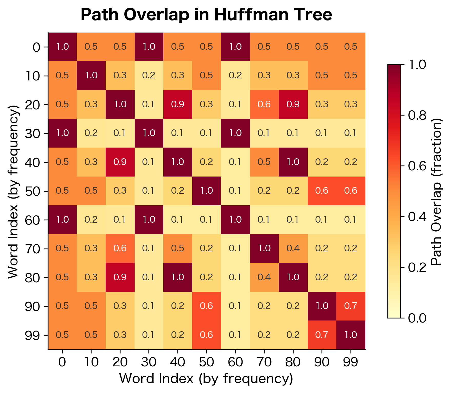
Path Overlap and Similarity
Consider two words and with paths that share a common prefix. The shared internal nodes must satisfy both words' training signals. This creates an implicit constraint: words with overlapping paths have representations that work well with the same internal node vectors.
Huffman coding places similar-frequency words nearby in the tree, so they share more path nodes. The path overlap analysis reveals that words with similar frequencies tend to share more path nodes in the Huffman tree. Words with vastly different frequencies (like 0 and 99) share fewer nodes since they're placed at different depths. This frequency-based grouping has interesting implications for learning, as discussed below.
The Curse of Random Trees
With random tree structures (or balanced trees), word placements are arbitrary. A cat and a dog might be far apart in the tree, while a cat and a verb might be nearby. This mismatch between tree structure and semantic similarity can hurt embedding quality.
The Huffman tree partially addresses this: it groups words by frequency, not semantics, but frequently co-occurring words often share semantic domains. More sophisticated approaches construct trees based on word similarity (using pre-trained embeddings or co-occurrence statistics), placing semantically similar words near each other in the tree.
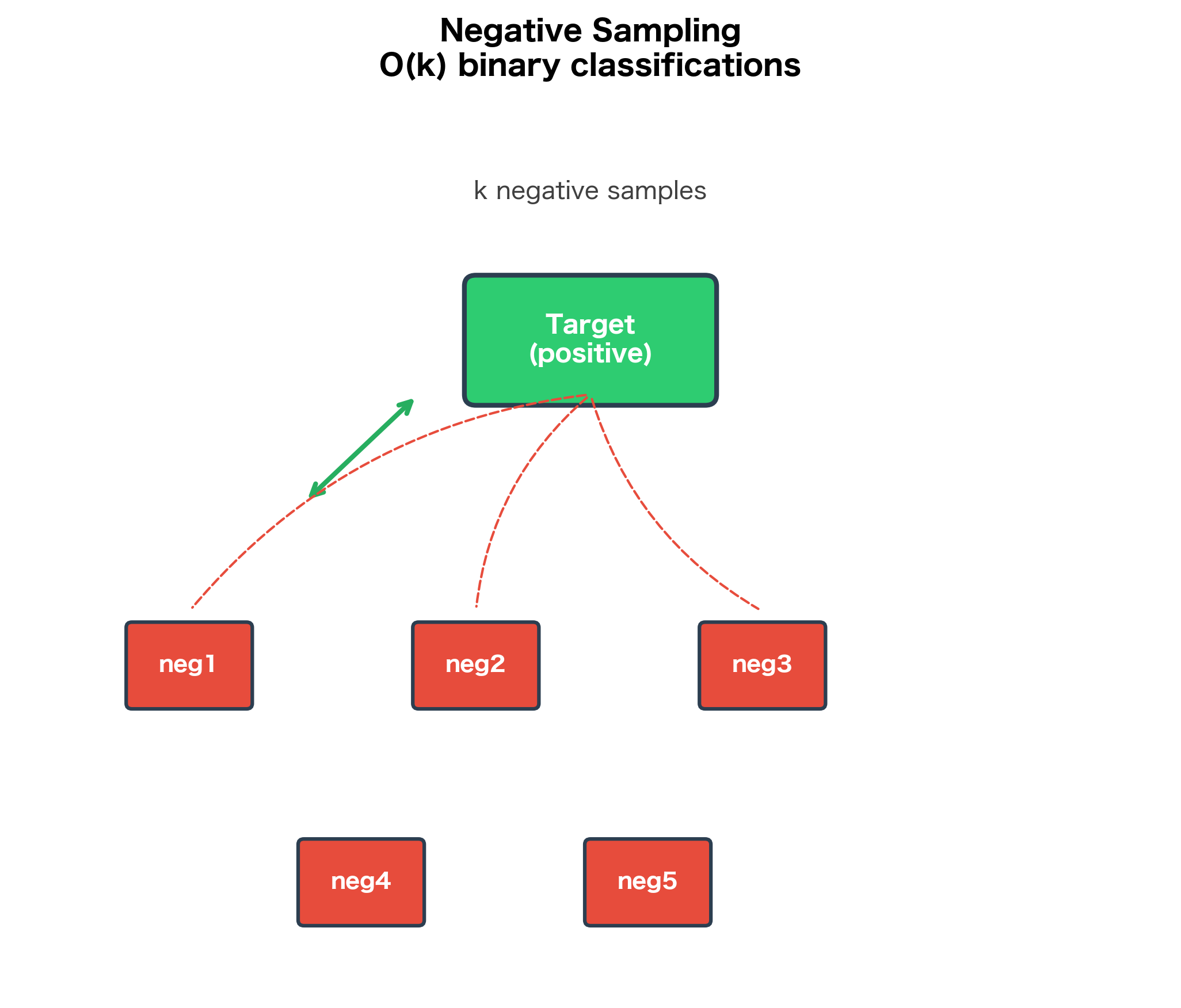
Hierarchical Softmax vs Negative Sampling
Both hierarchical softmax and negative sampling solve the same problem: making Skip-gram training tractable. How do they compare?
| Aspect | Hierarchical Softmax | Negative Sampling |
|---|---|---|
| Complexity | per word | per word ( = number of negatives) |
| Probability model | Exact probabilities (sum to 1) | Approximate (sigmoid on pairs) |
| Rare words | Equal treatment regardless of frequency | May underrepresent very rare words |
| Tree structure | Huffman tree required | No special structure |
| Implementation | More complex (tree traversal) | Simpler (random sampling) |
| Gradient quality | Gradients from all path nodes | Gradients from sampled negatives only |
When to Use Each Approach
Hierarchical Softmax works well when:
- You need proper probability distributions over words
- You want consistent treatment of rare words
- The vocabulary structure is meaningful (can be encoded in tree)
- Memory for tree structure is available
Negative Sampling is preferred when:
- Training speed is the primary concern
- The vocabulary is very large ()
- Simple implementation is important
- You're learning representations (not probability estimates)
In practice, negative sampling is more commonly used in modern Word2Vec implementations due to its simplicity and comparable embedding quality. However, hierarchical softmax remains valuable for understanding the theoretical foundations and for applications requiring proper probability estimates.
Limitations and Considerations
Hierarchical softmax has important limitations to understand:
-
Tree structure sensitivity: The quality of learned embeddings depends on tree construction. A poorly structured tree (where semantically similar words are far apart) can hurt performance. Huffman coding optimizes for computation, not semantics.
-
Fixed tree structure: Once built, the tree is static. Adding new words requires rebuilding the tree and potentially retraining. This makes hierarchical softmax less suitable for dynamic vocabularies.
-
Gradient distribution: All internal nodes on a word's path receive gradient updates. For deep paths, gradients may be small by the time they reach root-level nodes. This is analogous to vanishing gradients in deep networks.
-
Memory overhead: Storing the tree structure and node vectors requires additional memory. For a vocabulary of words, there are internal nodes, each with an embedding-dimensional vector.
-
Implementation complexity: Tree traversal and path lookup add complexity compared to the straightforward sampling in negative sampling.
Key Parameters
Understanding the key parameters in hierarchical softmax helps when implementing or tuning the algorithm:
| Parameter | Description | Typical Values | Impact |
|---|---|---|---|
embedding_dim | Dimension of word and node vectors | 50-300 | Higher dimensions capture more nuance but increase memory and computation |
learning_rate | Step size for gradient updates | 0.01-0.5 | Higher rates speed training but may cause instability; often decayed during training |
word_freqs | Word frequency distribution | From corpus | Determines Huffman tree structure; accurate frequencies yield optimal path lengths |
vocab_size | Number of words in vocabulary | 10K-500K | Affects tree depth () and memory requirements ( internal nodes) |
Additional considerations for implementation:
-
Tree Construction: The Huffman tree is built once before training based on word frequencies. Using accurate corpus frequencies is important. If frequencies don't match the actual training distribution, the tree won't be optimal.
-
Initialization: Node vectors are typically initialized with small random values (e.g.,
np.random.randn(dim) * 0.01). Too-large initial values can cause sigmoid saturation, leading to vanishing gradients. -
Learning Rate Scheduling: Like most neural network training, hierarchical softmax benefits from learning rate decay. Starting with a higher rate (0.1-0.5) and decreasing linearly or exponentially during training often improves final embedding quality.
Summary
Hierarchical softmax transforms the expensive softmax computation into an efficient tree traversal. By organizing the vocabulary as a binary tree, each word's probability becomes a product of binary decisions along its path from root to leaf.
Key takeaways:
- Binary tree structure: Each word is a leaf; internal nodes have learned vectors that determine left/right decisions
- Path probability: where encodes direction
- Huffman coding: Assigns frequent words to short paths, reducing average computation. The expected path length is minimized
- Gradient computation: Each path node receives updates proportional to its prediction error. The input embedding receives accumulated gradients from all path nodes
- Complexity reduction: From to per training example, enabling training on large vocabularies
- Trade-offs: More complex than negative sampling; tree structure affects learned representations; proper probabilities (unlike negative sampling)
The next chapter explores negative sampling, an alternative approximation that achieves similar computational benefits with a simpler implementation. Understanding both approaches provides insight into the computational challenges of training language models and the clever solutions that make them practical.
Quiz
Ready to test your understanding? Take this quick quiz to reinforce what you've learned about hierarchical softmax.

Comments