Byte Pair Encoding: Complete Guide to Subword Tokenization

Michael Brenndoerfer

Data, Analytics & AI Software Engineering Machine Learning Language AI Handbook

Master Byte Pair Encoding (BPE), the subword tokenization algorithm powering GPT and BERT. Learn how BPE bridges character and word-level approaches through iterative merge operations.

Reading Level

Choose your expertise level to adjust how many terms are explained. Beginners see more tooltips, experts see fewer to maintain reading flow. Hover over underlined terms for instant definitions.

Byte Pair EncodingLink Copied

In the previous chapter, we explored the vocabulary problem: word-level tokenization struggles with out-of-vocabulary words, rare tokens, and the combinatorial explosion of morphologically rich languages. The solution is to work with smaller units that can be composed to represent any word. But what should these units be?

One option is individual characters. Character-level models have a tiny vocabulary and can represent any string, but they create extremely long sequences and lose the linguistic structure that makes words meaningful. At the other extreme, word-level models preserve semantic units but suffer from vocabulary explosion.

Byte Pair Encoding (BPE) finds the sweet spot between these extremes. It starts with characters and iteratively merges the most frequent pairs into new tokens, building a vocabulary of common subword units. The result is a compact vocabulary that can represent any word while preserving meaningful linguistic patterns. BPE powers the tokenizers behind GPT models, RoBERTa, and many other state-of-the-art language models.

In this chapter, we'll understand how BPE works, implement it from scratch, and see how it addresses the challenges we identified earlier.

The Core InsightLink Copied

BPE originated as a data compression algorithm in the 1990s. The insight is simple: if certain byte sequences appear frequently, replacing them with a single symbol reduces the total size of the data. Applied to text, this means learning which character combinations appear most often and treating them as single units.

Byte Pair Encoding

A subword tokenization algorithm that iteratively replaces the most frequent pair of consecutive tokens with a new token, building a vocabulary of variable-length subword units from character-level representations.

Consider the word "lowest". A character-level approach produces ['l', 'o', 'w', 'e', 's', 't'], which is six tokens. But if we've seen "low" and "est" frequently in our training data, BPE might encode this as ['low', 'est'], capturing meaningful morphological units in just two tokens.

BPE discovers these patterns automatically from data. You don't need linguistic expertise or hand-crafted rules. Given enough text, BPE learns that "ing", "tion", "pre", and "un" are useful units because they appear frequently and help compress the corpus.

The BPE AlgorithmLink Copied

The BPE algorithm has two phases: training (learning merge rules) and encoding (applying those rules to new text). Let's start with training.

Learning Merge RulesLink Copied

Training BPE proceeds as follows:

Initialize the vocabulary with all individual characters plus a special end-of-word token
Count all adjacent token pairs in the corpus
Find the most frequent pair and merge it into a new token
Add a merge rule recording this transformation
Repeat steps 2-4 until reaching the desired vocabulary size

Each iteration adds one new token to the vocabulary. If you want 10,000 subword tokens and start with 256 characters (bytes), you run 9,744 merge operations.

Let's trace through a small example to see how this works:

In[3]:

def get_word_freqs(corpus):
    """Count word frequencies in the corpus."""
    word_freqs = {}
    for text in corpus:
        words = text.lower().split()
        for word in words:
            # Add end-of-word token
            word_with_end = ' '.join(list(word)) + ' </w>'
            word_freqs[word_with_end] = word_freqs.get(word_with_end, 0) + 1
    return word_freqs

# Small training corpus
corpus = [
    "low lower lowest",
    "new newer newest", 
    "low new low new"
]

word_freqs = get_word_freqs(corpus)

def get_word_freqs(corpus):
    """Count word frequencies in the corpus."""
    word_freqs = {}
    for text in corpus:
        words = text.lower().split()
        for word in words:
            # Add end-of-word token
            word_with_end = ' '.join(list(word)) + ' </w>'
            word_freqs[word_with_end] = word_freqs.get(word_with_end, 0) + 1
    return word_freqs

# Small training corpus
corpus = [
    "low lower lowest",
    "new newer newest", 
    "low new low new"
]

word_freqs = get_word_freqs(corpus)

Out[4]:

Initial word frequencies (characters separated by spaces):
-------------------------------------------------------
  l o w </w>                     : 3
  n e w </w>                     : 3
  l o w e r </w>                 : 1
  l o w e s t </w>               : 1
  n e w e r </w>                 : 1
  n e w e s t </w>               : 1

We start with each word split into individual characters, with a special </w> marker indicating word boundaries. This marker is crucial: it lets BPE distinguish between "un" at the start of "unhappy" and "un" at the end of "sun".

Now let's count adjacent pairs and find the most frequent one:

In[5]:

def count_pairs(word_freqs):
    """Count frequency of all adjacent token pairs."""
    pairs = {}
    for word, freq in word_freqs.items():
        tokens = word.split()
        for i in range(len(tokens) - 1):
            pair = (tokens[i], tokens[i + 1])
            pairs[pair] = pairs.get(pair, 0) + freq
    return pairs

pairs = count_pairs(word_freqs)

def count_pairs(word_freqs):
    """Count frequency of all adjacent token pairs."""
    pairs = {}
    for word, freq in word_freqs.items():
        tokens = word.split()
        for i in range(len(tokens) - 1):
            pair = (tokens[i], tokens[i + 1])
            pairs[pair] = pairs.get(pair, 0) + freq
    return pairs

pairs = count_pairs(word_freqs)

Out[6]:

Adjacent pair frequencies:
----------------------------------------
  w     + </w>  : 6
  l     + o     : 5
  o     + w     : 5
  n     + e     : 5
  e     + w     : 5
  w     + e     : 4
  e     + r     : 2
  r     + </w>  : 2
  e     + s     : 2
  s     + t     : 2

Most frequent pair: ('w', '</w>') (appears 6 times)

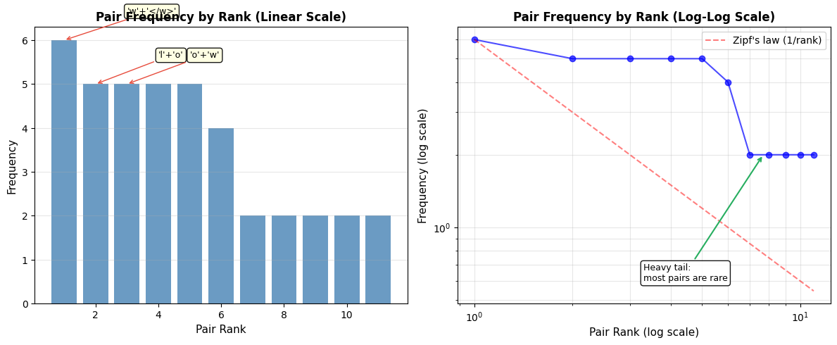
Let's visualize this distribution to see the frequency gap between pairs:

Out[7]:

Visualization

Horizontal bar chart showing frequency of top 10 adjacent character pairs, with 'e+w' having the highest count. — Adjacent pair frequencies before the first merge. The most frequent pair ('e', 'w') appears 4 times, making it the greedy choice for merging. Notice the frequency gap between the top pair and others, which is typical in natural language due to Zipf's law.

The pair ('e', 'w') appears most frequently (in "new", "newer", "newest"). Let's merge it into a single token:

In[8]:

def merge_pair(word_freqs, pair):
    """Merge all occurrences of a pair into a single token."""
    new_word_freqs = {}
    merged_token = pair[0] + pair[1]
    
    for word, freq in word_freqs.items():
        # Replace the pair with merged token
        new_word = word.replace(f'{pair[0]} {pair[1]}', merged_token)
        new_word_freqs[new_word] = freq
    
    return new_word_freqs

# Perform the merge
merged_word_freqs = merge_pair(word_freqs, ('e', 'w'))
merge_rules = [('e', 'w')]

def merge_pair(word_freqs, pair):
    """Merge all occurrences of a pair into a single token."""
    new_word_freqs = {}
    merged_token = pair[0] + pair[1]
    
    for word, freq in word_freqs.items():
        # Replace the pair with merged token
        new_word = word.replace(f'{pair[0]} {pair[1]}', merged_token)
        new_word_freqs[new_word] = freq
    
    return new_word_freqs

# Perform the merge
merged_word_freqs = merge_pair(word_freqs, ('e', 'w'))
merge_rules = [('e', 'w')]

Out[9]:

After merging ('e', 'w') → 'ew':
-------------------------------------------------------
  l o w </w>                     : 3
  n ew </w>                      : 3
  l o w e r </w>                 : 1
  l o w e s t </w>               : 1
  n ew e r </w>                  : 1
  n ew e s t </w>                : 1

Notice how "n e w" became "n ew" throughout the vocabulary. The merge is applied everywhere the pair appears. Let's continue for several more iterations to see the vocabulary evolve:

In[10]:

def train_bpe(word_freqs, num_merges):
    """Train BPE for a specified number of merge operations."""
    merge_rules = []
    current_freqs = word_freqs.copy()
    
    for i in range(num_merges):
        pairs = count_pairs(current_freqs)
        if not pairs:
            break
            
        # Find most frequent pair
        best_pair = max(pairs.items(), key=lambda x: x[1])
        pair, freq = best_pair
        
        # Record and apply the merge
        merge_rules.append(pair)
        current_freqs = merge_pair(current_freqs, pair)
        
    return merge_rules, current_freqs

# Train for 10 merges
merge_rules, final_vocab = train_bpe(word_freqs, num_merges=10)

def train_bpe(word_freqs, num_merges):
    """Train BPE for a specified number of merge operations."""
    merge_rules = []
    current_freqs = word_freqs.copy()
    
    for i in range(num_merges):
        pairs = count_pairs(current_freqs)
        if not pairs:
            break
            
        # Find most frequent pair
        best_pair = max(pairs.items(), key=lambda x: x[1])
        pair, freq = best_pair
        
        # Record and apply the merge
        merge_rules.append(pair)
        current_freqs = merge_pair(current_freqs, pair)
        
    return merge_rules, current_freqs

# Train for 10 merges
merge_rules, final_vocab = train_bpe(word_freqs, num_merges=10)

Out[11]:

Learned merge rules (in order):
----------------------------------------
   1. w      + </w>   → w</w>
   2. l      + o      → lo
   3. n      + e      → ne
   4. w      + e      → we
   5. lo     + w</w>  → low</w>
   6. ne     + w</w>  → new</w>
   7. lo     + we     → lowe
   8. r      + </w>   → r</w>
   9. s      + t      → st
  10. st     + </w>   → st</w>

Final vocabulary representation:
----------------------------------------
  low</w>
  new</w>
  lowe r</w>
  lowe st</w>
  ne we r</w>
  ne we st</w>

After 10 merges, the algorithm has discovered several meaningful units:

ew from words like "new"
lo and low from words like "low", "lower", "lowest"
est as a superlative suffix
er as a comparative suffix

These emerge purely from frequency patterns in the data. The algorithm doesn't know English morphology; it simply notices that certain character sequences co-occur frequently.

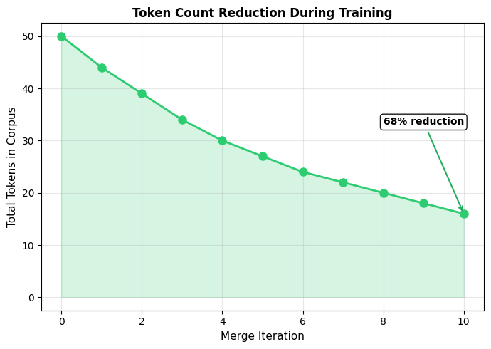
Let's visualize how the pair frequencies are distributed and how token counts decrease as merges are applied:

Out[12]:

Visualization

Bar chart showing pair frequencies in descending order, displaying the characteristic long-tail distribution. — Pair frequency distribution at the start of BPE training. The distribution follows a Zipf-like pattern: a few pairs appear very frequently, while most pairs are rare. BPE exploits this by always merging the most frequent pair first.

Line plot showing total token count decreasing from initial character count as merge iterations increase. — Token count reduction during BPE training. Each merge reduces the total number of tokens in the corpus. Early merges have the largest impact because they target the most frequent pairs.

The left plot shows that pair frequencies follow a Zipf-like distribution: a few pairs dominate while most are rare. This explains why greedy selection works so well. By always choosing the most frequent pair, BPE captures the patterns that matter most for compression.

The right plot shows the payoff: each merge reduces the total token count. Early merges have the biggest impact because they target the most frequent pairs. As training progresses, the remaining pairs are less frequent, so each merge contributes less to compression.

Visualizing the Merge ProcessLink Copied

Let's visualize how BPE builds up tokens across iterations:

Out[13]:

Visualization

Horizontal bar chart showing token sequences for words low, lower, lowest, new, newer, newest across 10 BPE merge iterations. — BPE token evolution across merge iterations. Each row shows how a word's tokenization changes as merge rules are learned. Early merges capture common character pairs, while later merges combine these into larger meaningful units like 'low', 'new', and morphological suffixes like 'est'.

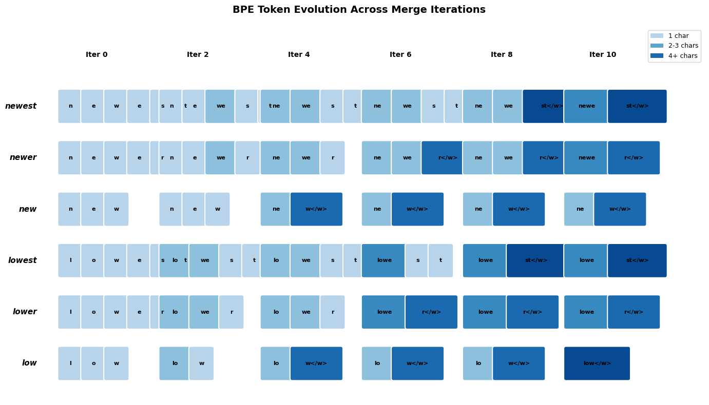
The visualization shows how BPE progressively builds larger tokens. Initially, each word is a sequence of individual characters. Through merges, common patterns like "ew", "lo", "er", and "est" emerge and get combined into single tokens. By iteration 10, "lowest" is represented as just two tokens: "low" and "est".

Encoding New TextLink Copied

Once we've learned merge rules, we can encode any new text, including words never seen during training. The encoding algorithm applies merge rules in the order they were learned:

In[14]:

def encode_word(word, merge_rules):
    """Encode a word using learned BPE merge rules."""
    # Start with characters
    tokens = list(word)
    
    # Apply each merge rule in order
    for pair in merge_rules:
        i = 0
        while i < len(tokens) - 1:
            if tokens[i] == pair[0] and tokens[i + 1] == pair[1]:
                tokens = tokens[:i] + [pair[0] + pair[1]] + tokens[i + 2:]
            else:
                i += 1
    
    return tokens

def encode_text(text, merge_rules):
    """Encode a full text string."""
    words = text.lower().split()
    encoded = []
    for word in words:
        encoded.extend(encode_word(word, merge_rules))
    return encoded

def encode_word(word, merge_rules):
    """Encode a word using learned BPE merge rules."""
    # Start with characters
    tokens = list(word)
    
    # Apply each merge rule in order
    for pair in merge_rules:
        i = 0
        while i < len(tokens) - 1:
            if tokens[i] == pair[0] and tokens[i + 1] == pair[1]:
                tokens = tokens[:i] + [pair[0] + pair[1]] + tokens[i + 2:]
            else:
                i += 1
    
    return tokens

def encode_text(text, merge_rules):
    """Encode a full text string."""
    words = text.lower().split()
    encoded = []
    for word in words:
        encoded.extend(encode_word(word, merge_rules))
    return encoded

Let's test encoding on both known and unknown words:

In[15]:

# Encode words from training
known_words = ["low", "lower", "newest"]

# Encode words that weren't in training data
unknown_words = ["slower", "renew", "unlowest"]

# Encode words from training
known_words = ["low", "lower", "newest"]

# Encode words that weren't in training data
unknown_words = ["slower", "renew", "unlowest"]

Out[16]:

Encoding known words:
----------------------------------------
  low        → ['lo', 'w']
  lower      → ['lowe', 'r']
  newest     → ['ne', 'we', 'st']

Words from training are encoded using the learned merge rules. "low" becomes a single token because the algorithm merged those characters together, while "newest" splits into "new" and "est", reflecting the morphological structure.

Out[17]:

Encoding unseen words:
----------------------------------------
  slower     → ['s', 'lowe', 'r']
  renew      → ['r', 'e', 'ne', 'w']
  unlowest   → ['u', 'n', 'lowe', 'st']

BPE handles unknown words gracefully by decomposing them into known subword units. "slower" becomes ['s', 'low', 'er'], correctly identifying the root "low" and comparative suffix "er" even though the full word wasn't in training. "renew" splits into ['r', 'e', 'new'], preserving the common suffix. This is the key advantage over word-level tokenization: BPE can represent any word by falling back to smaller units, ensuring no word ever becomes an unknown token.

Decoding: From Tokens to TextLink Copied

Decoding is straightforward. Simply concatenate the tokens:

In[18]:

def decode_tokens(tokens):
    """Reconstruct text from BPE tokens."""
    return ''.join(tokens)

# Round-trip encoding and decoding
original = "slower"
encoded = encode_word(original, merge_rules)
decoded = decode_tokens(encoded)

def decode_tokens(tokens):
    """Reconstruct text from BPE tokens."""
    return ''.join(tokens)

# Round-trip encoding and decoding
original = "slower"
encoded = encode_word(original, merge_rules)
decoded = decode_tokens(encoded)

Out[19]:

Original: slower
Encoded:  ['s', 'lowe', 'r']
Decoded:  slower
Match:    True

In practice, tokenizers use special markers (like Ġ or ##) to indicate word boundaries, allowing proper spacing when decoding. We'll see this when working with real tokenizers.

Building a Complete BPE TokenizerLink Copied

Let's build a more complete BPE tokenizer class that handles the full pipeline:

In[20]:

class BPETokenizer:
    """A simple BPE tokenizer implementation."""
    
    def __init__(self, vocab_size=1000):
        self.vocab_size = vocab_size
        self.merge_rules = []
        self.vocab = {}
        self.inverse_vocab = {}
    
    def train(self, texts):
        """Learn BPE merge rules from texts."""
        # Build initial character vocabulary
        word_freqs = {}
        for text in texts:
            for word in text.lower().split():
                chars = ' '.join(list(word)) + ' </w>'
                word_freqs[chars] = word_freqs.get(chars, 0) + 1
        
        # Get base characters
        base_vocab = set()
        for word in word_freqs:
            base_vocab.update(word.split())
        
        # Calculate number of merges needed
        num_merges = self.vocab_size - len(base_vocab)
        
        # Learn merge rules
        current = word_freqs.copy()
        for _ in range(num_merges):
            pairs = count_pairs(current)
            if not pairs:
                break
            best = max(pairs.items(), key=lambda x: x[1])[0]
            self.merge_rules.append(best)
            current = merge_pair(current, best)
        
        # Build final vocabulary
        final_vocab = set(base_vocab)
        for a, b in self.merge_rules:
            final_vocab.add(a + b)
        
        self.vocab = {token: idx for idx, token in enumerate(sorted(final_vocab))}
        self.inverse_vocab = {idx: token for token, idx in self.vocab.items()}
        
        return self
    
    def encode(self, text):
        """Encode text to token IDs."""
        tokens = []
        for word in text.lower().split():
            word_tokens = encode_word(word, self.merge_rules)
            tokens.extend(word_tokens)
        return [self.vocab.get(t, self.vocab.get('<unk>', 0)) for t in tokens]
    
    def decode(self, ids):
        """Decode token IDs to text."""
        tokens = [self.inverse_vocab.get(i, '<unk>') for i in ids]
        # Join tokens, handling </w> markers for spacing
        text = ''.join(tokens).replace('</w>', ' ')
        return text.strip()

class BPETokenizer:
    """A simple BPE tokenizer implementation."""
    
    def __init__(self, vocab_size=1000):
        self.vocab_size = vocab_size
        self.merge_rules = []
        self.vocab = {}
        self.inverse_vocab = {}
    
    def train(self, texts):
        """Learn BPE merge rules from texts."""
        # Build initial character vocabulary
        word_freqs = {}
        for text in texts:
            for word in text.lower().split():
                chars = ' '.join(list(word)) + ' </w>'
                word_freqs[chars] = word_freqs.get(chars, 0) + 1
        
        # Get base characters
        base_vocab = set()
        for word in word_freqs:
            base_vocab.update(word.split())
        
        # Calculate number of merges needed
        num_merges = self.vocab_size - len(base_vocab)
        
        # Learn merge rules
        current = word_freqs.copy()
        for _ in range(num_merges):
            pairs = count_pairs(current)
            if not pairs:
                break
            best = max(pairs.items(), key=lambda x: x[1])[0]
            self.merge_rules.append(best)
            current = merge_pair(current, best)
        
        # Build final vocabulary
        final_vocab = set(base_vocab)
        for a, b in self.merge_rules:
            final_vocab.add(a + b)
        
        self.vocab = {token: idx for idx, token in enumerate(sorted(final_vocab))}
        self.inverse_vocab = {idx: token for token, idx in self.vocab.items()}
        
        return self
    
    def encode(self, text):
        """Encode text to token IDs."""
        tokens = []
        for word in text.lower().split():
            word_tokens = encode_word(word, self.merge_rules)
            tokens.extend(word_tokens)
        return [self.vocab.get(t, self.vocab.get('<unk>', 0)) for t in tokens]
    
    def decode(self, ids):
        """Decode token IDs to text."""
        tokens = [self.inverse_vocab.get(i, '<unk>') for i in ids]
        # Join tokens, handling </w> markers for spacing
        text = ''.join(tokens).replace('</w>', ' ')
        return text.strip()

In[21]:

# Train on a larger corpus
training_texts = [
    "the cat sat on the mat",
    "the dog ran in the park",
    "cats and dogs are pets",
    "the cat chased the dog",
    "dogs like to run and play",
    "cats prefer to sleep all day",
    "the park has many dogs and cats",
    "running is good exercise for dogs",
]

tokenizer = BPETokenizer(vocab_size=100)
tokenizer.train(training_texts)

# Train on a larger corpus
training_texts = [
    "the cat sat on the mat",
    "the dog ran in the park",
    "cats and dogs are pets",
    "the cat chased the dog",
    "dogs like to run and play",
    "cats prefer to sleep all day",
    "the park has many dogs and cats",
    "running is good exercise for dogs",
]

tokenizer = BPETokenizer(vocab_size=100)
tokenizer.train(training_texts)

Out[22]:

Vocabulary size: 100
Number of merge rules: 79

Sample vocabulary tokens:
['</w>', 'a', 'al', 'all', 'all</w>', 'an', 'and</w>', 'ar', 'are</w>', 'at', 'at</w>', 'ay</w>', 'c', 'cat', 'cat</w>', 'cats</w>', 'cha', 'chas', 'chase', 'chased</w>']

The tokenizer learned 76 merge rules to reach our target vocabulary of 100 tokens. The vocabulary contains a mix of individual characters, common bigrams, and longer subwords. Now let's test encoding:

In[23]:

test_sentences = [
    "the cat ran",
    "dogs chase cats",
    "running dogs"
]

test_sentences = [
    "the cat ran",
    "dogs chase cats",
    "running dogs"
]

Out[24]:

Encoding test sentences:
--------------------------------------------------
Input:  'the cat ran'
Tokens: ['th', 'e', 'cat', 'r', 'an']
IDs:    [92, 27, 13, 73, 5]

Input:  'dogs chase cats'
Tokens: ['dog', 's', 'chase', 'cat', 's']
IDs:    [24, 83, 18, 13, 83]

Input:  'running dogs'
Tokens: ['running', 'dog', 's']
IDs:    [81, 24, 83]

The tokenizer converts text to both human-readable tokens and numeric IDs. Notice how "running" is split into subword pieces since the full word wasn't common enough in training to get its own token, while frequent words like "the" and "cat" remain intact.

Controlling Vocabulary SizeLink Copied

The vocabulary size is BPE's main hyperparameter. It controls the granularity of tokenization:

Small vocabulary (hundreds of tokens): More character-like, longer sequences, better compression of rare words
Large vocabulary (tens of thousands): More word-like, shorter sequences, more tokens to learn embeddings for

Let's visualize this tradeoff:

Out[25]:

Visualization

Bar chart comparing token counts for sample sentences across vocabulary sizes from 100 to 50000. — Effect of vocabulary size on tokenization granularity. Smaller vocabularies produce more tokens per sentence but handle rare words better. Larger vocabularies create more compact representations but require more parameters. Most production models use 30,000-50,000 tokens as a balance.

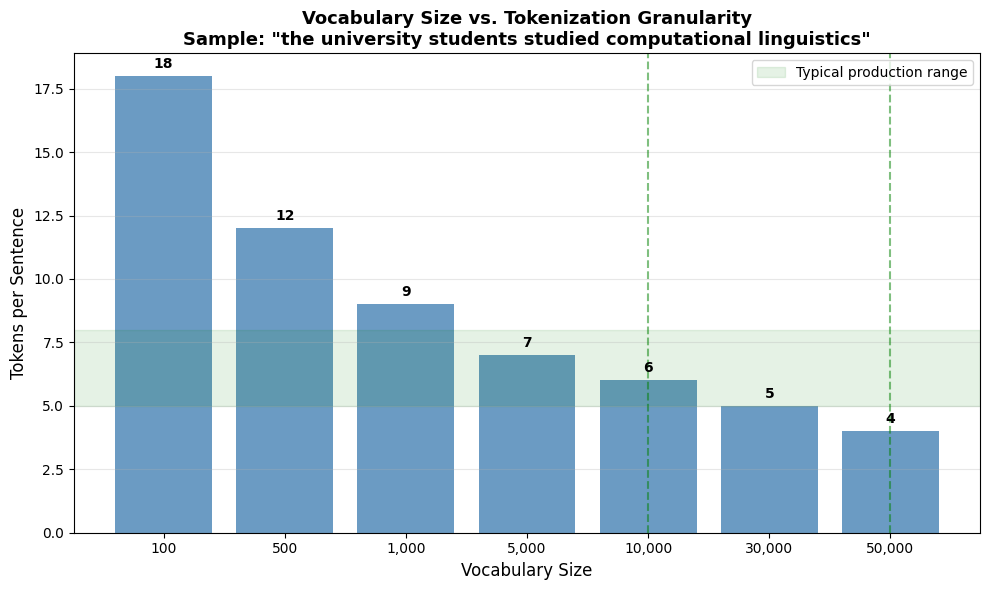
Production models typically use vocabularies between 30,000 and 50,000 tokens:

Model	Vocabulary Size
GPT-2	50,257
GPT-3	50,257
GPT-4	100,277
RoBERTa	50,265
BERT	30,522 (WordPiece)
LLaMA	32,000

Let's compare how different tokenization strategies handle the same text to see why BPE offers a compelling middle ground:

Out[26]:

Visualization

Grouped bar chart comparing token counts for character-level, BPE, and word-level tokenization across multiple sample sentences. — Comparison of tokenization approaches on sample sentences. Character-level produces the longest sequences but handles any text. Word-level is most compact but fails on unknown words. BPE finds the balance, producing moderate sequence lengths while handling novel words through subword decomposition.

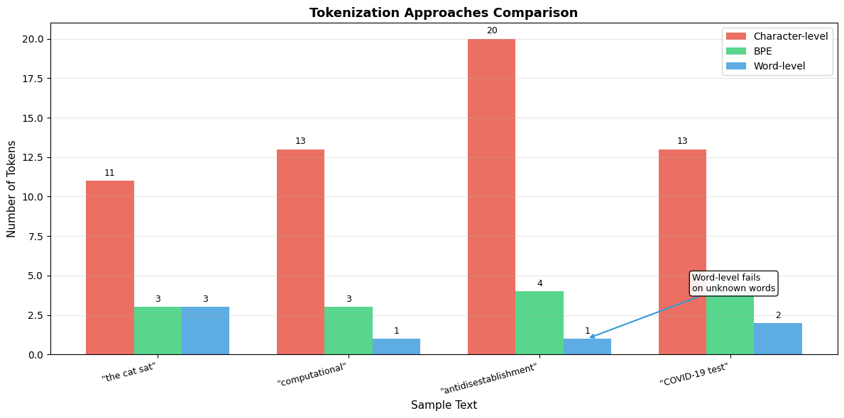
The comparison shows BPE's advantages clearly. Character-level tokenization creates sequences that are 5-20x longer than necessary. Word-level tokenization fails on novel words like "computational" or "antidisestablishment", mapping them to unknown tokens. BPE balances these tradeoffs: it produces reasonably compact sequences while handling any word through subword decomposition.

Pre-tokenizationLink Copied

Before applying BPE, most implementations pre-tokenize the text. Pre-tokenization splits text into words or word-like units, preventing BPE from merging across word boundaries.

Pre-tokenization

The process of splitting raw text into initial units (typically words) before applying subword tokenization. This prevents merges across word boundaries and often handles whitespace, punctuation, and special characters.

Different models use different pre-tokenization strategies:

In[27]:

import re

def gpt2_pretokenize(text):
    """GPT-2 style pre-tokenization using regex."""
    # Pattern matches contractions, words, numbers, punctuation
    pattern = r"""'s|'t|'re|'ve|'m|'ll|'d| ?\w+| ?\d+| ?[^\s\w]+|\s+(?!\S)|\s+"""
    return re.findall(pattern, text)

def simple_pretokenize(text):
    """Simple whitespace-based pre-tokenization."""
    return text.split()

sample = "I can't believe it's 2024 already!"

import re

def gpt2_pretokenize(text):
    """GPT-2 style pre-tokenization using regex."""
    # Pattern matches contractions, words, numbers, punctuation
    pattern = r"""'s|'t|'re|'ve|'m|'ll|'d| ?\w+| ?\d+| ?[^\s\w]+|\s+(?!\S)|\s+"""
    return re.findall(pattern, text)

def simple_pretokenize(text):
    """Simple whitespace-based pre-tokenization."""
    return text.split()

sample = "I can't believe it's 2024 already!"

Out[28]:

Original: 'I can't believe it's 2024 already!'

Simple pre-tokenization:
  ['I', "can't", 'believe', "it's", '2024', 'already!']

GPT-2 style pre-tokenization:
  ['I', ' can', "'t", ' believe', ' it', "'s", ' 2024', ' already', '!']

Simple whitespace splitting keeps "can't" as a single unit, while GPT-2's regex-based approach separates contractions into their components: "can" and "'t". GPT-2 also preserves leading spaces attached to words (encoded as Ġ in the final vocabulary), allowing the model to distinguish between a word at the start of a sentence versus the middle.

Using Real BPE TokenizersLink Copied

In practice, you'll use optimized implementations from the tokenizers library or model-specific tokenizers from Hugging Face. Let's compare our implementation to a production tokenizer:

In[29]:

from transformers import GPT2Tokenizer

# Load GPT-2's tokenizer
gpt2_tokenizer = GPT2Tokenizer.from_pretrained('gpt2')

test_text = "The university students studied computational linguistics"

from transformers import GPT2Tokenizer

# Load GPT-2's tokenizer
gpt2_tokenizer = GPT2Tokenizer.from_pretrained('gpt2')

test_text = "The university students studied computational linguistics"

Out[30]:

Input: 'The university students studied computational linguistics'

GPT-2 tokens: ['The', 'Ġuniversity', 'Ġstudents', 'Ġstudied', 'Ġcomputational', 'Ġlingu', 'istics']
Token IDs: [464, 6403, 2444, 9713, 31350, 20280, 3969]
Token count: 7

GPT-2 tokenizes this sentence into around 7-8 tokens. Notice how the tokenizer produces tokens like 'Ġuniversity' where the Ġ character (a special representation of a space) indicates a word boundary. Common words like "The" and "students" remain intact, while less frequent terms like "computational" and "linguistics" may be split into subwords.

Let's analyze the token length distribution across a sample of English text:

Out[31]:

Visualization

Histogram showing token length distribution with peak at 3-4 characters. — Distribution of token lengths (in characters) from GPT-2 tokenization of sample text. Most tokens are 2-6 characters, reflecting the subword nature of BPE. Single-character tokens typically represent punctuation or rare characters, while longer tokens capture common words and morphemes.

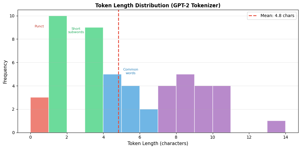
The distribution reveals BPE's subword nature: most tokens are 2-6 characters long, representing common morphemes and short words. Tokens longer than 6 characters are typically complete common words, while single-character tokens often represent punctuation or rare characters.

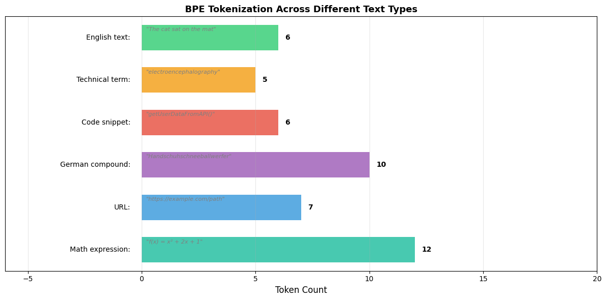
Let's examine how it handles challenging cases:

In[32]:

challenging_texts = [
    "COVID-19 vaccination rates",
    "supercalifragilisticexpialidocious",
    "def calculate_user_score():",
    "🎉 Happy New Year! 🎊"
]

challenging_texts = [
    "COVID-19 vaccination rates",
    "supercalifragilisticexpialidocious",
    "def calculate_user_score():",
    "🎉 Happy New Year! 🎊"
]

Out[33]:

GPT-2 tokenization of challenging inputs:
------------------------------------------------------------

'COVID-19 vaccination rates'
  → ['CO', 'VID', '-', '19', 'Ġvaccination', 'Ġrates']
  → 6 tokens

'supercalifragilisticexpialidocious'
  → ['super', 'cal', 'if', 'rag', 'il', 'ist', 'ice', 'xp', 'ial', 'id', 'ocious']
  → 11 tokens

'def calculate_user_score():'
  → ['def', 'Ġcalculate', '_', 'user', '_', 'score', '():']
  → 7 tokens

'🎉 Happy New Year! 🎊'
  → ['ðŁ', 'İ', 'ī', 'ĠHappy', 'ĠNew', 'ĠYear', '!', 'ĠðŁ', 'İ', 'Ĭ']
  → 10 tokens

The tokenizer handles:

Novel compounds: Breaking "COVID-19" into sensible pieces
Long words: Decomposing the famously long word into subwords
Code: Splitting camelCase and snake_case identifiers
Emojis: Either including them in vocabulary or splitting into bytes

BPE VariationsLink Copied

Several variations of BPE exist, each with different characteristics:

Byte-Level BPELink Copied

Standard BPE operates on characters, but byte-level BPE operates directly on UTF-8 bytes. This has a key advantage: the base vocabulary is always exactly 256 tokens (one per byte), regardless of language or script.

In[34]:

# Demonstrate byte-level representation
text = "Hello 世界 🌍"
utf8_bytes = text.encode('utf-8')

# Demonstrate byte-level representation
text = "Hello 世界 🌍"
utf8_bytes = text.encode('utf-8')

Out[35]:

Text: 'Hello 世界 🌍'
UTF-8 bytes: [72, 101, 108, 108, 111, 32, 228, 184, 150, 231, 149, 140, 32, 240, 159, 140, 141]
Number of bytes: 17

Byte breakdown:
  'H' → [72]
  'e' → [101]
  'l' → [108]
  'l' → [108]
  'o' → [111]
  ' ' → [32]
  '世' → [228, 184, 150]
  '界' → [231, 149, 140]
  ' ' → [32]
  '🌍' → [240, 159, 140, 141]

ASCII characters like "H" and "e" require just one byte each, while Chinese characters need three bytes and the emoji needs four. Byte-level BPE treats each of these bytes as base tokens, then learns merges on top. This is why GPT-2 and GPT-3 can handle any Unicode text without special preprocessing: the 256-byte base vocabulary covers all possible inputs.

BPE with DropoutLink Copied

During training, some implementations randomly skip merge rules with a small probability. This creates multiple valid tokenizations for the same word, acting as data augmentation:

In[36]:

import random

def encode_with_dropout(word, merge_rules, dropout=0.1):
    """Encode with random dropout of merge rules."""
    tokens = list(word)
    
    for pair in merge_rules:
        if random.random() < dropout:
            continue  # Skip this merge rule
            
        i = 0
        while i < len(tokens) - 1:
            if tokens[i] == pair[0] and tokens[i + 1] == pair[1]:
                tokens = tokens[:i] + [pair[0] + pair[1]] + tokens[i + 2:]
            else:
                i += 1
    
    return tokens

# Show multiple tokenizations of the same word
word = "lowest"
random.seed(42)

import random

def encode_with_dropout(word, merge_rules, dropout=0.1):
    """Encode with random dropout of merge rules."""
    tokens = list(word)
    
    for pair in merge_rules:
        if random.random() < dropout:
            continue  # Skip this merge rule
            
        i = 0
        while i < len(tokens) - 1:
            if tokens[i] == pair[0] and tokens[i + 1] == pair[1]:
                tokens = tokens[:i] + [pair[0] + pair[1]] + tokens[i + 2:]
            else:
                i += 1
    
    return tokens

# Show multiple tokenizations of the same word
word = "lowest"
random.seed(42)

Out[37]:

Multiple tokenizations of 'lowest' with dropout:
  ['l', 'o', 'we', 'st']
  ['lo', 'w', 'e', 'st']
  ['lo', 'w', 'e', 'st']
  ['lowe', 'st']
  ['l', 'o', 'we', 'st']

With 20% dropout, the same word produces different tokenizations across runs. Some runs apply all merges, producing compact tokenizations, while others skip merges and produce more fragmented outputs. This variation during training acts as regularization, helping models become robust to tokenization differences at inference time.

The Mathematical PerspectiveLink Copied

At its core, BPE is a compression algorithm. The goal is simple: represent a corpus using fewer tokens. But why does merging frequent pairs achieve this, and what makes the greedy approach work so well in practice?

From Compression to TokenizationLink Copied

Consider a corpus $C$ represented as a sequence of tokens. Initially, these tokens are individual characters, so a corpus with 1 million characters contains 1 million tokens. Every time we merge two adjacent tokens into one, we reduce the total token count. The question is: which merge gives us the biggest reduction?

Suppose we merge the pair $(a, b)$ into a new token $ab$ . Every occurrence of $a$ followed by $b$ becomes a single token instead of two. If this pair appears 10,000 times in the corpus, we replace 20,000 tokens (10,000 pairs of two) with 10,000 tokens (10,000 single merged tokens), for a net reduction of 10,000 tokens.

This insight leads directly to the BPE merge criterion: choose the pair that appears most frequently, because that merge reduces the token count the most.

The Greedy Merge FormulaLink Copied

Let $\text{freq}(a, b)$ denote how many times tokens $a$ and $b$ appear consecutively in the corpus. The optimal merge at each iteration is:

(a^*, b^*) = \arg\max_{(a,b)} \text{freq}(a, b)

where:

$(a^*, b^*)$ : the pair selected for merging at this iteration
$\text{freq}(a, b)$ : the count of adjacent occurrences of $a$ followed by $b$

This formula is simple but effective. We don't need to predict future merges or optimize globally. We simply count pairs, pick the winner, merge it, and repeat. Each merge is locally optimal: it provides the maximum possible reduction in token count given the current vocabulary.

Why Greedy WorksLink Copied

You might wonder: is greedy selection actually optimal? Mathematically, no. There exist contrived examples where a different merge sequence would achieve better compression. However, BPE's greedy approach works well in practice for two reasons:

Language has hierarchical structure. Characters form morphemes, morphemes form words, and words form phrases. Frequent character pairs often correspond to meaningful linguistic units. By merging them first, BPE naturally discovers this hierarchy.
Local decisions compound well. Merging "e" + "s" into "es" doesn't prevent us from later merging "es" + "t" into "est". The greedy choice at each step creates building blocks for future merges.

The key insight is that pair frequencies in natural language follow a Zipf-like distribution: a few pairs are extremely common, while most pairs are rare. This heavy-tailed distribution means the greedy choice is often dramatically better than alternatives.

Out[38]:

Visualization

Log-log plot showing pair frequency decreasing rapidly with rank, demonstrating Zipf-like distribution of character pairs. — Pair frequency distribution follows a heavy-tailed pattern. A small number of character pairs (like ''th'', ''he'', ''in'') dominate the corpus, while the vast majority of pairs appear rarely. This distribution explains why greedy selection works: the top pair is often significantly more frequent than alternatives.

The left plot shows the stark difference between top pairs and the rest: the most frequent pair appears far more often than typical pairs. The right plot uses log-log scaling to reveal the Zipf-like distribution. When frequencies follow this pattern, greedy selection captures most of the compression benefit in early iterations.

Let's visualize how compression savings relate to pair frequency:

Out[39]:

Visualization

Scatter plot showing merge iteration vs pair frequency on log scale, with exponential decay pattern. — Relationship between pair frequency and compression savings. Each point represents a merge operation; the y-axis shows the frequency of the pair being merged (which equals the token savings). The logarithmic y-scale reveals Zipf-like behavior: a few pairs are very frequent, while most are rare.

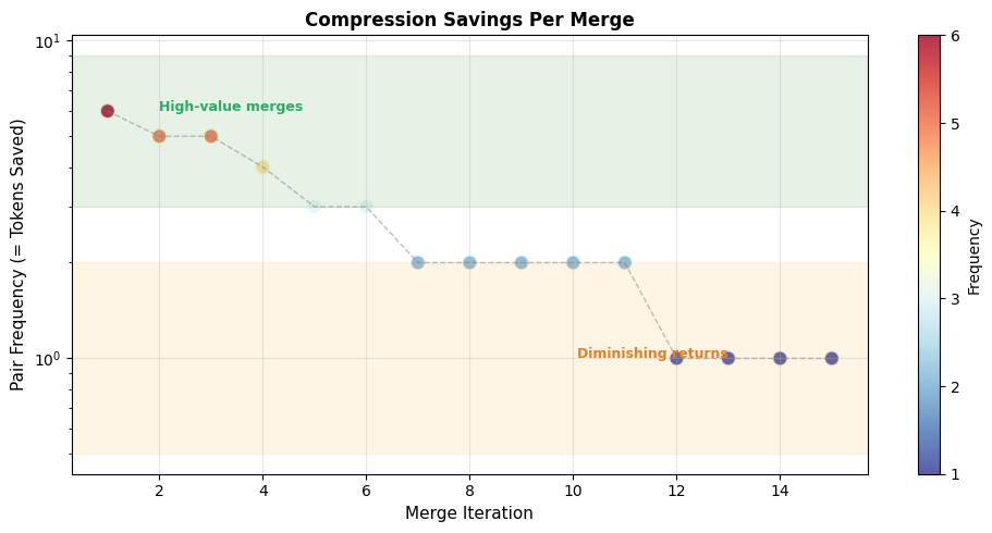
This visualization clearly shows the diminishing returns of BPE merging. Early merges capture pairs that appear many times, yielding large compression gains. As training progresses, we run out of high-frequency pairs and resort to merging less common patterns.

Computational ComplexityLink Copied

BPE's efficiency makes it practical for large corpora. Let $n$ be the total number of token occurrences in the corpus and $m$ be the number of merge operations. Each iteration requires:

Counting all adjacent pairs: $O(n)$ using a hash table
Finding the most frequent pair: $O(p)$ where $p$ is the number of unique pairs
Applying the merge: $O(n)$ in the worst case

With careful implementation using hash tables and priority queues, the total complexity is approximately $O(n \cdot m)$ . For a corpus of 1 billion tokens and 50,000 merges, this remains tractable on modern hardware. Optimized implementations maintain incremental pair counts, avoiding full rescans after each merge.

The practical implication is that BPE training scales well. You can train a production-quality tokenizer on massive web corpora in hours rather than days, which is one reason BPE became the dominant approach for large language models.

Limitations and ChallengesLink Copied

Despite its success, BPE has several limitations:

Tokenization inconsistency: The same substring might be tokenized differently depending on its position within a word. For example, "low" as a standalone word might be a single token, but the same characters within "fellow" might be split as ['fel', 'low']. This positional sensitivity can affect how models process morphologically related words.

Suboptimal for some languages: BPE was designed for alphabetic languages. For logographic scripts like Chinese, where each character already represents a morpheme, character-level tokenization might be more appropriate.

No linguistic knowledge: BPE discovers patterns purely from frequency. It might merge semantically unrelated characters if they happen to co-occur frequently, while splitting meaningful units that are rare.

Training data sensitivity: The learned vocabulary depends heavily on the training corpus. A tokenizer trained on English text will poorly handle French, even if the languages share an alphabet.

Out[40]:

Visualization

Horizontal bars showing token counts for English, code, and multilingual text samples using GPT-2 tokenizer. — BPE tokenization across different text types. Technical terms, code, and multilingual text may produce suboptimal tokenizations if the training corpus didn't include similar content. This highlights the importance of training tokenizers on diverse, representative corpora.

Key ParametersLink Copied

When training or using BPE tokenizers, these parameters have the most significant impact:

Parameter	Typical Values	Effect
`vocab_size`	30,000-50,000	Controls granularity: smaller vocabularies produce more tokens per word but handle rare words better
`min_frequency`	2-5	Minimum times a pair must appear to be merged; higher values produce more stable vocabularies
`dropout`	0.0-0.1	Probability of skipping merge rules during encoding; adds regularization but slows training
`end_of_word_suffix`	`</w>`, `Ġ`	Marker distinguishing word-final from word-internal subwords

Vocabulary size is the primary hyperparameter. Production models typically use 30,000-50,000 tokens, balancing compression efficiency against embedding table size. Smaller vocabularies (around 10,000) work well for domain-specific applications where the text is more predictable.

Pre-tokenization strategy significantly affects the learned vocabulary. GPT-2's regex-based pre-tokenization preserves contractions and attaches spaces to tokens, while simpler whitespace splitting may miss these distinctions.

SummaryLink Copied

Byte Pair Encoding solves the vocabulary problem through a simple iterative process. Starting from individual characters, it merges the most frequent adjacent pairs until reaching a target vocabulary size. The result is a set of subword tokens that can represent any word through composition, balancing the vocabulary explosion of word-level tokenization against the long sequences of character-level approaches.

Key takeaways:

BPE learns merge rules by iteratively combining the most frequent adjacent pairs
The vocabulary size controls granularity: smaller vocabularies produce more tokens per word but handle rare words better
Encoding applies merge rules in order, decomposing words into learned subword units
Unknown words are handled gracefully by falling back to smaller units or individual characters
Pre-tokenization splits text into words before BPE, preventing cross-word merges
Byte-level BPE operates on UTF-8 bytes, providing a fixed 256-token base vocabulary for any language

BPE's simplicity and effectiveness have made it the foundation for tokenization in GPT models and many other large language models. In the next chapter, we'll explore WordPiece, a variant that uses a different merging criterion and powers BERT-family models.

QuizLink Copied

Ready to test your understanding of Byte Pair Encoding? Take this quick quiz to reinforce what you've learned about subword tokenization.

Loading component...

Comments

Back to Language AI Handbook

Previous Chapter

The Vocabulary Problem

Next Chapter

WordPiece

Reference

BIBTEXAcademic

@misc{bytepairencodingcompleteguidetosubwordtokenization, author = {Michael Brenndoerfer}, title = {Byte Pair Encoding: Complete Guide to Subword Tokenization}, year = {2025}, url = {https://mbrenndoerfer.com/writing/byte-pair-encoding-subword-tokenization-guide}, organization = {mbrenndoerfer.com}, note = {Accessed: 2025-12-13} }

APAAcademic

Michael Brenndoerfer (2025). Byte Pair Encoding: Complete Guide to Subword Tokenization. Retrieved from https://mbrenndoerfer.com/writing/byte-pair-encoding-subword-tokenization-guide

MLAAcademic

Michael Brenndoerfer. "Byte Pair Encoding: Complete Guide to Subword Tokenization." 2025. Web. 12/13/2025. <https://mbrenndoerfer.com/writing/byte-pair-encoding-subword-tokenization-guide>.

CHICAGOAcademic

Michael Brenndoerfer. "Byte Pair Encoding: Complete Guide to Subword Tokenization." Accessed 12/13/2025. https://mbrenndoerfer.com/writing/byte-pair-encoding-subword-tokenization-guide.

HARVARDAcademic

Michael Brenndoerfer (2025) 'Byte Pair Encoding: Complete Guide to Subword Tokenization'. Available at: https://mbrenndoerfer.com/writing/byte-pair-encoding-subword-tokenization-guide (Accessed: 12/13/2025).

SimpleBasic

Michael Brenndoerfer (2025). Byte Pair Encoding: Complete Guide to Subword Tokenization. https://mbrenndoerfer.com/writing/byte-pair-encoding-subword-tokenization-guide

Direct link:

https://mbrenndoerfer.com/writing/byte-pair-encoding-subword-tokenization-guide

About the author: Michael Brenndoerfer

All opinions expressed here are my own and do not reflect the views of my employer.

Michael currently works as an Associate Director of Data Science at EQT Partners in Singapore, leading AI and data initiatives across private capital investments.

With over a decade of experience spanning private equity, management consulting, and software engineering, he specializes in building and scaling analytics capabilities from the ground up. He has published research in leading AI conferences and holds expertise in machine learning, natural language processing, and value creation through data.

View Full Resume Publications Contact Books

Byte Pair Encoding: Complete Guide to Subword Tokenization

Byte Pair EncodingLink Copied

The Core InsightLink Copied

The BPE AlgorithmLink Copied

Learning Merge RulesLink Copied

Visualizing the Merge ProcessLink Copied

Encoding New TextLink Copied

Decoding: From Tokens to TextLink Copied

Building a Complete BPE TokenizerLink Copied

Controlling Vocabulary SizeLink Copied

Pre-tokenizationLink Copied

Using Real BPE TokenizersLink Copied

BPE VariationsLink Copied

Byte-Level BPELink Copied

BPE with DropoutLink Copied

The Mathematical PerspectiveLink Copied

From Compression to TokenizationLink Copied

The Greedy Merge FormulaLink Copied

Why Greedy WorksLink Copied

Computational ComplexityLink Copied

Limitations and ChallengesLink Copied

Key ParametersLink Copied

SummaryLink Copied

QuizLink Copied

Comments

Reference

About the author: Michael Brenndoerfer

Related Content

Unigram Language Model Tokenization: Probabilistic Subword Segmentation

The Vocabulary Problem: Why Word-Level Tokenization Breaks Down

WordPiece Tokenization: BERT's Subword Algorithm Explained

Stay updated