

Master SVD for NLP, including truncated SVD for dimensionality reduction, Latent Semantic Analysis, and randomized SVD for large-scale text processing.

This article is part of the free-to-read Language AI Handbook
Choose your expertise level to adjust how many terms are explained. Beginners see more tooltips, experts see fewer to maintain reading flow. Hover over underlined terms for instant definitions.
Singular Value Decomposition
Co-occurrence matrices capture the distributional patterns that reveal word meaning. But these matrices have a problem: they're enormous and mostly empty. A vocabulary of 100,000 words produces a matrix with 10 billion entries, yet most word pairs never co-occur. This sparsity makes storage expensive, computation slow, and similarity estimates unreliable.
Singular Value Decomposition (SVD) solves this by finding a compact representation that preserves the essential structure. Instead of storing billions of sparse counts, we extract a few hundred dense dimensions that capture the underlying semantic patterns. This is the mathematical foundation behind Latent Semantic Analysis (LSA) and a conceptual precursor to modern word embeddings.
The Intuition: Finding Hidden Structure
Consider a term-document matrix where rows are words and columns are documents. Each entry counts how often a word appears in a document. This matrix is high-dimensional (one dimension per document) and sparse (most words don't appear in most documents).
But the underlying semantic structure is much simpler. Documents about "cars" tend to mention "engine," "wheel," "drive," and "road" together. Documents about "cooking" cluster words like "recipe," "ingredient," "stir," and "oven." These latent topics create correlations: knowing a document contains "engine" makes "wheel" more likely.
SVD discovers these hidden patterns. It finds a small number of dimensions that explain most of the variance in the data. Words that co-occur with similar patterns end up close together in this reduced space, even if they never directly co-occurred in the original matrix.
SVD is a matrix factorization that decomposes any matrix into three matrices: . The columns of and are orthonormal bases, and is a diagonal matrix of singular values that indicate the importance of each dimension.
The Mathematics of SVD
To understand SVD, we need to answer a fundamental question: what does it mean to decompose a matrix? And more importantly, why would we want to?
The Core Problem: Too Much Information, Poorly Organized
Consider our term-document matrix . Each entry tells us how often word appears in document . This is raw information, accurate but overwhelming. With 100,000 words and 10,000 documents, we have a billion numbers, most of them zeros. Worse, this representation treats each document as an independent dimension, ignoring the obvious fact that documents about similar topics should be similar.
What we want is a compressed representation that:
- Captures the essential patterns (words that co-occur, documents that are similar)
- Discards the noise (random co-occurrences that don't reflect meaning)
- Organizes information along meaningful dimensions
SVD achieves all three by factoring the matrix into simpler pieces that reveal its underlying structure.
Building Toward the Decomposition
Let's develop the SVD formula by thinking about what we need. Our matrix has size , where is the vocabulary size and is the number of documents (or vocabulary size for word-word matrices).
Step 1: Find the principal directions.
The first insight is that not all directions in our data space are equally important. Some directions capture major patterns (the "technology vs. cooking" distinction), while others capture noise. We want to identify these directions and rank them by importance.
Mathematically, we're looking for orthogonal directions, perpendicular axes that don't interfere with each other. These will become our new coordinate system.
Step 2: Measure importance along each direction.
Once we have the directions, we need to know how much the data varies along each one. A direction with high variance captures important structure; one with low variance captures noise.
Step 3: Express everything in terms of these new coordinates.
Finally, we rewrite our original matrix using the new directions and their importances. This is the decomposition.
The SVD Formula
SVD accomplishes all three steps in one elegant factorization:
Each component has a specific role:
| Component | Size | Role |
|---|---|---|
| Word directions: orthogonal vectors describing how words relate to latent dimensions | ||
| Importance scores: diagonal matrix of singular values | ||
| Document directions: orthogonal vectors describing how documents relate to latent dimensions |
The singular values are always non-negative and sorted in decreasing order. The number of non-zero singular values, , equals the rank of the matrix, the true dimensionality of the information it contains.
Why orthogonality matters. The conditions and ensure that each column of is perpendicular to every other column (and likewise for ). This orthogonality makes the dimensions independent, each capturing a distinct pattern. Without orthogonality, dimensions would overlap and we couldn't cleanly separate signal from noise.
Geometric Interpretation: A New Coordinate System
Think of SVD as discovering the natural coordinate system for your data. The original matrix transforms vectors from an -dimensional input space to an -dimensional output space. SVD reveals that this transformation has three distinct phases:
- Rotate the input space using to align with the principal directions of variation
- Scale each dimension by its singular value , stretching important directions and shrinking unimportant ones
- Rotate again using to produce the final output
This decomposition is visualized below. The singular values tell us how much the matrix stretches along each principal direction:
- Large : The data varies greatly along this direction, capturing important structure
- Small : Little variation, likely noise or fine details we can safely ignore
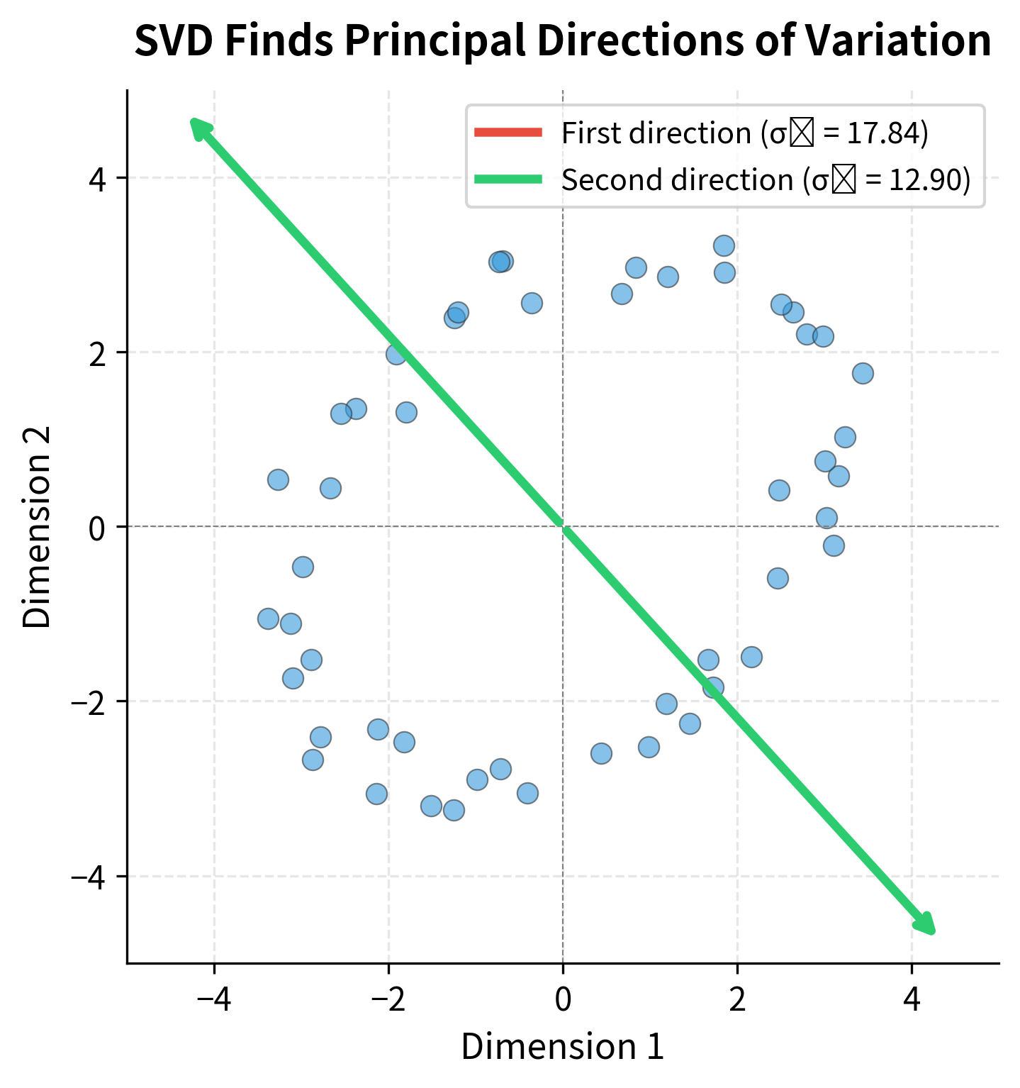
The visualization demonstrates the key insight: most of the data's spread lies along the first principal direction. The second direction captures much less variation. If we kept only the first direction, we'd lose some information, but we'd preserve the dominant pattern. This observation leads directly to the most powerful application of SVD.
Truncated SVD: Keeping What Matters
Full SVD computes all singular values and vectors, but we rarely need them all. In practice, we keep only the top components, dramatically reducing dimensionality while preserving most of the meaningful structure. This truncated version is the form most useful for NLP applications.
The Insight: Most Information Lives in Few Dimensions
Here's the remarkable fact that makes SVD useful for NLP: real data is approximately low-rank. A term-document matrix with millions of entries might have its essential structure captured by just a few hundred dimensions. The remaining dimensions contain noise, rare events, and idiosyncratic details.
Why does this happen? Because language has structure:
- Documents about technology share vocabulary, creating correlated columns
- Words with similar meanings appear in similar contexts, creating correlated rows
- Topics, genres, and writing styles impose patterns that span many entries
These correlations mean the matrix isn't truly dimensional. It's effectively much smaller. SVD reveals this hidden simplicity.
The Truncated SVD Formula
If we keep only the largest singular values and discard the rest, we get:
The components are truncated versions of the full decomposition:
| Component | Original Size | Truncated Size | What's Kept |
|---|---|---|---|
| First columns (most important word directions) | |||
| Top singular values (largest importances) | |||
| First rows (most important document directions) |
This isn't just any approximation. It's the best possible rank- approximation.
Among all matrices with rank at most , the truncated SVD minimizes the reconstruction error (Frobenius norm). No other rank- matrix can get closer to the original. This mathematical guarantee is why SVD is the gold standard for linear dimensionality reduction.
Quantifying Information Loss
How much information do we lose by keeping only dimensions? The singular values provide an exact answer. Since each represents the variance captured by dimension , the fraction of total variance explained by the top dimensions is:
where:
- : the -th singular value (importance of dimension )
- : the number of dimensions we choose to retain
- : the rank of the original matrix (total non-zero singular values)
The key insight: In text data, this ratio typically rises quickly. The first few dimensions might capture 50% of the variance, the first 50 might capture 80%, and the first 200 might capture 95%. The remaining thousands of dimensions contribute almost nothing.
This rapid concentration of variance is why dimensionality reduction works so well for language. The semantic structure we care about lives in a low-dimensional subspace.
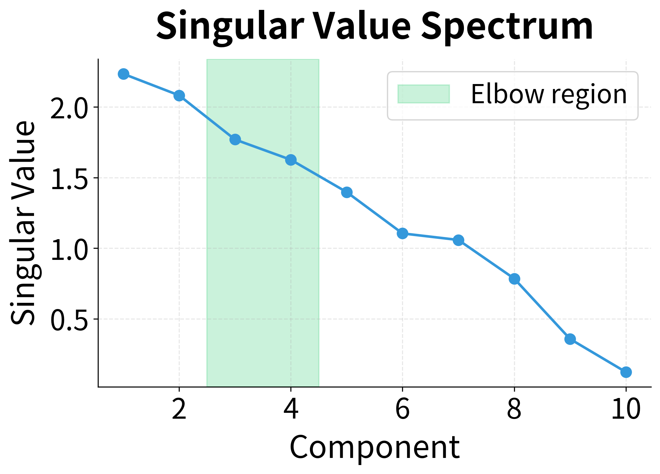
Notice the dramatic gap between the first three singular values and the rest. This isn't coincidence. We generated this data with exactly three hidden topics. The singular value spectrum has revealed this latent structure: three large values corresponding to the three topics, followed by much smaller values representing noise and fine-grained details.
This is the power of SVD for exploratory analysis: the singular value decay reveals the intrinsic dimensionality of your data. A sharp drop suggests clear underlying structure; a gradual decay suggests more complex, distributed patterns.
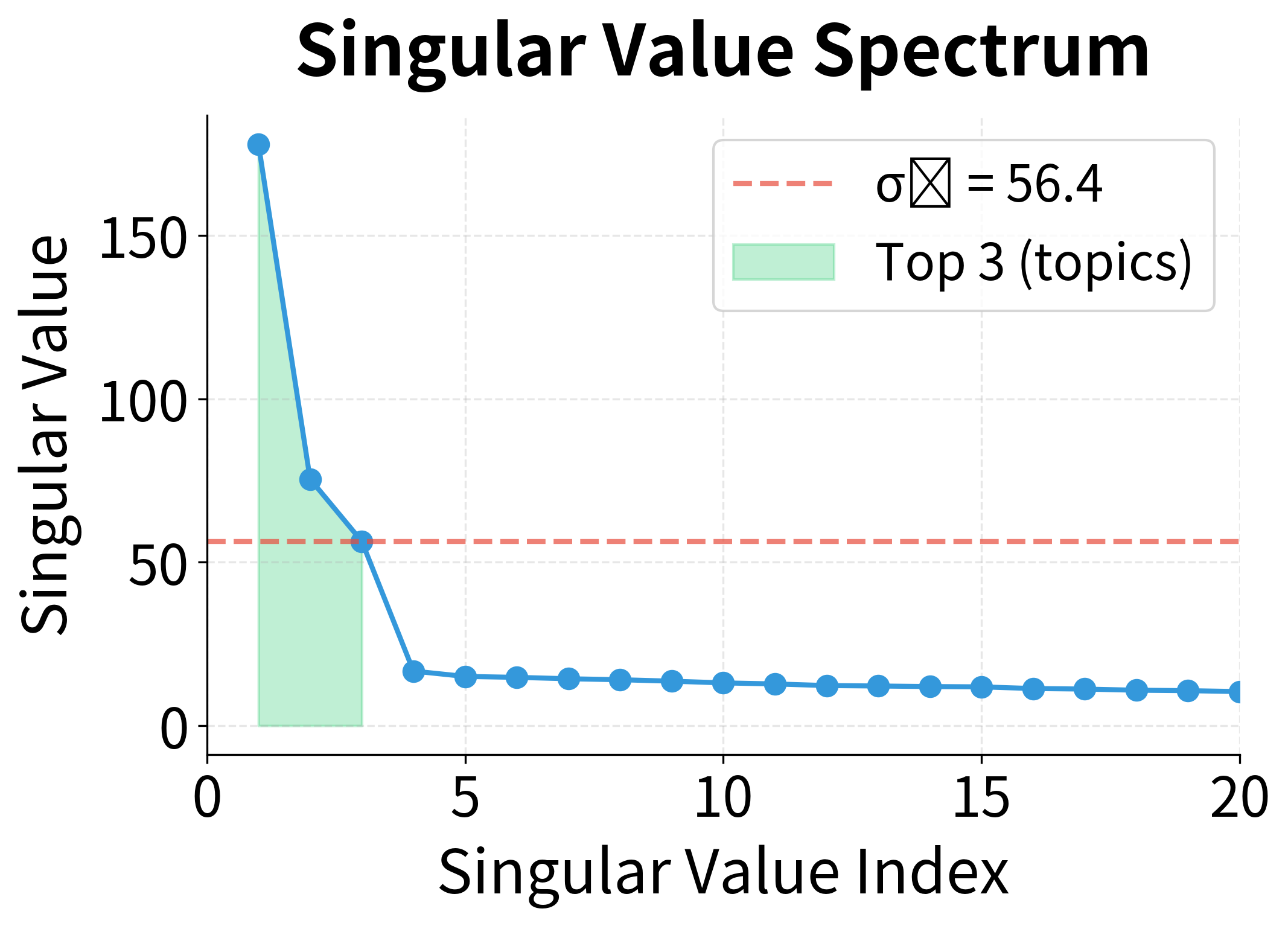
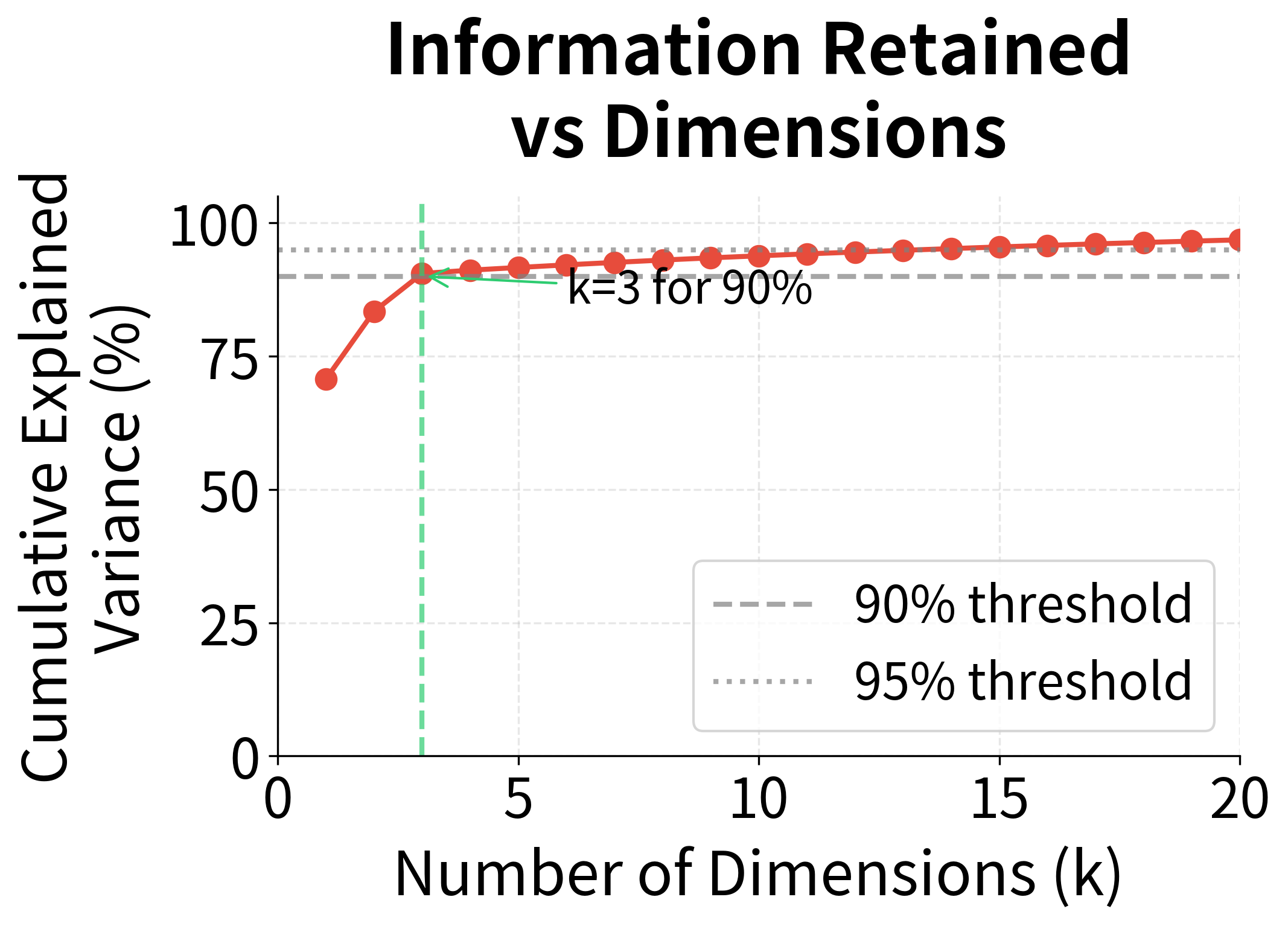
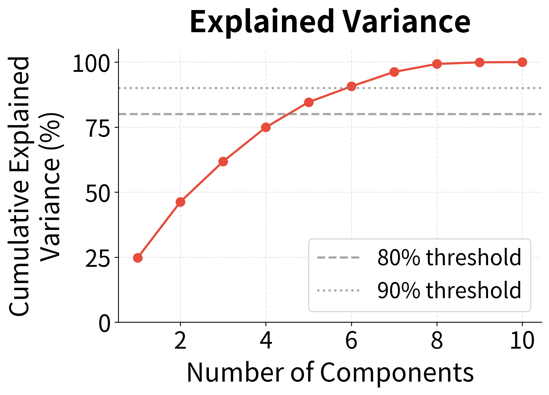
The left plot shows the singular value spectrum. Note how the first three values tower over the rest. The right plot translates this into cumulative explained variance: with just 10 dimensions, we've captured over 90% of the matrix's information. The annotation marks where we cross the 90% threshold, a common heuristic for choosing dimensionality.
In real text data, the decay is typically more gradual than this simulated example, but the principle holds: a small number of dimensions captures the semantic structure that matters.
Latent Semantic Analysis (LSA): From Theory to Practice
Now that we understand the mathematics of SVD, let's see how it transforms our understanding of text. Latent Semantic Analysis (LSA), introduced by Deerwester et al. in 1990, was one of the first successful methods for learning word representations, and it's built entirely on the truncated SVD we just developed.
The Central Insight
LSA rests on a powerful observation: the reduced SVD dimensions aren't arbitrary; they correspond to latent semantic concepts.
Consider what happens when we apply truncated SVD to a term-document matrix:
- Words that appear in similar documents get projected to similar locations
- Documents about similar topics get projected to similar locations
- The dimensions themselves often correspond to interpretable "topics" or semantic contrasts
This means two words can be similar in LSA space even if they never directly co-occur, as long as they appear in similar contexts. "Car" and "automobile" might never appear in the same document, but if they appear in documents about the same topics, LSA will discover their similarity.
Building an LSA Model Step by Step
Let's implement LSA from scratch. By building each component ourselves, we'll develop intuition for how the mathematics translates into semantic understanding.
Our filtered vocabulary contains words that appear in at least two documents, a simple but effective way to focus on meaningful terms. Notice the mix: technology words ("data," "algorithms"), cooking words ("cooking," "fresh"), and general words ("the," "with"). This diversity will let us observe how LSA discovers semantic structure without being told what the categories are.
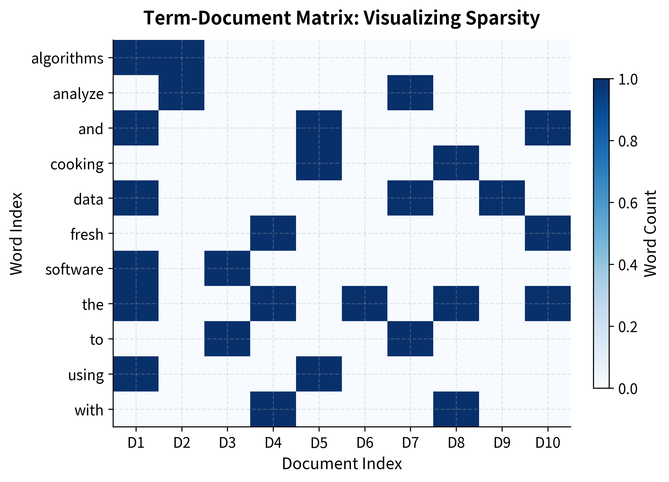
The heatmap reveals the sparsity pattern visually. Most cells are light (zero counts), with scattered darker cells where words actually appear in documents. This visual makes clear why storing and computing with the raw matrix is inefficient.
The matrix is extremely sparse. Most entries are zero because any given document contains only a tiny fraction of the vocabulary. This sparsity is both a curse and an opportunity:
- The curse: Sparse vectors are inefficient to store and compute with. Similarity calculations are unreliable when most dimensions are zero.
- The opportunity: The sparsity tells us the data is redundant. If most entries are predictable (zero), then the true information content is much smaller than the matrix size suggests.
SVD exploits this redundancy, compressing the sparse matrix into a dense representation that captures the underlying patterns.
Preprocessing: TF-IDF Weighting
Before applying SVD, we apply TF-IDF (Term Frequency-Inverse Document Frequency) weighting. This transformation addresses a subtle problem: raw counts overweight common words.
Words like "the" and "is" appear in nearly every document but carry little semantic information. TF-IDF down-weights these ubiquitous terms and up-weights distinctive words that characterize specific documents. The result is a matrix where the important patterns are more prominent.
Applying Truncated SVD: The Heart of LSA
Now comes the key step: we apply truncated SVD to extract the latent semantic dimensions. The function below computes the full SVD, then truncates to keep only the top components.
Important detail: Notice how we construct word and document vectors. For word vectors, we multiply by the singular values; for document vectors, we multiply by the singular values. This weighting ensures that more important dimensions contribute more to similarity calculations.
We've achieved our goal: each word is now represented by a dense 3-dimensional vector instead of a sparse 10-dimensional document vector. The singular values tell us the relative importance of each dimension. The first captures the most variance, the second captures the most of what remains, and so on.
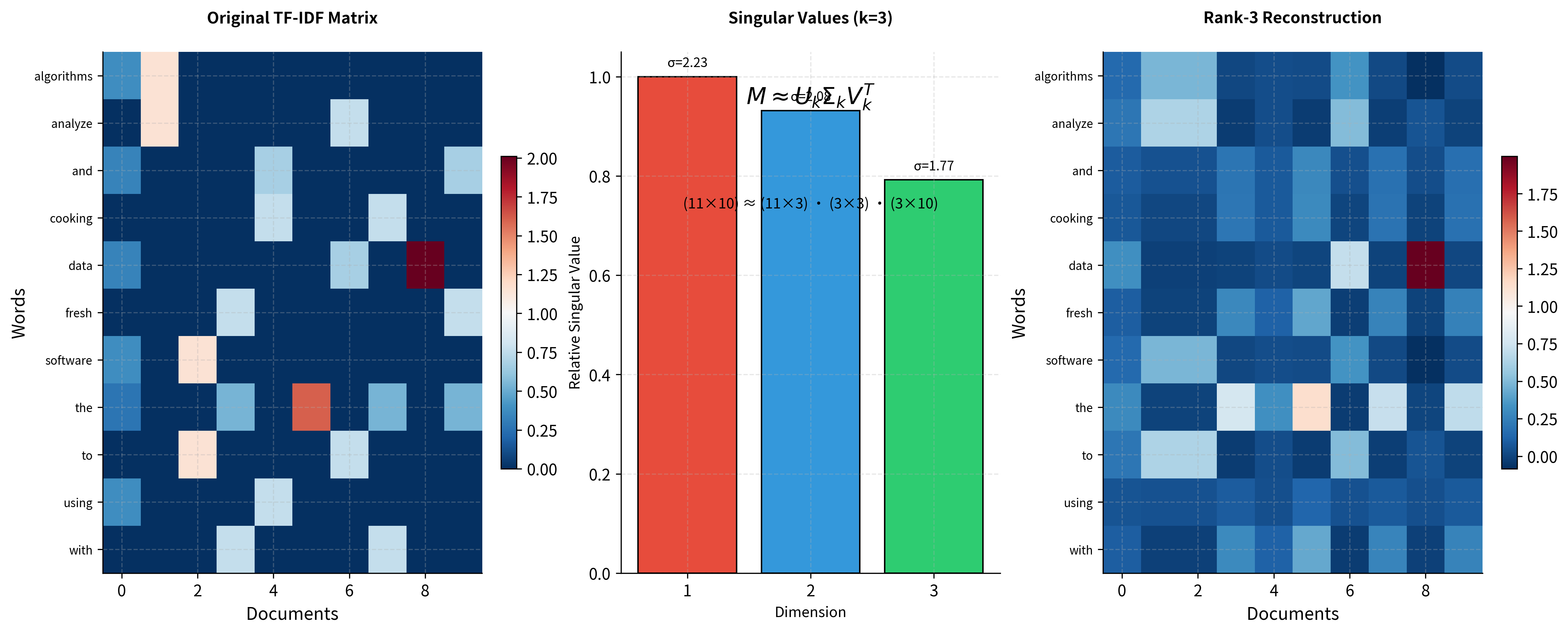
The visualization shows the SVD decomposition in action. The original matrix on the left contains the TF-IDF weighted word counts. The middle panel shows the singular values that weight each dimension. The reconstruction on the right shows what we get when we multiply the truncated components back together. The essential patterns are preserved while noise is smoothed out.
But what do these dimensions mean? This is where LSA becomes fascinating.
Interpreting the Latent Dimensions
Unlike hand-crafted features, SVD dimensions don't have predetermined meanings. But we can interpret them by examining which words load most strongly on each pole. A dimension might separate "technology vs. cooking," or "abstract vs. concrete," or capture some other semantic contrast that emerges from the data.
The output reveals interpretable structure. Each dimension has two poles, positive and negative loadings, and words cluster according to their semantic properties. Technology terms group together at one pole; cooking terms at another.
This is the magic of LSA: we never told the algorithm about "technology" or "cooking." It discovered these categories by analyzing which words appear in similar documents. The latent dimensions are emergent properties of the corpus structure.
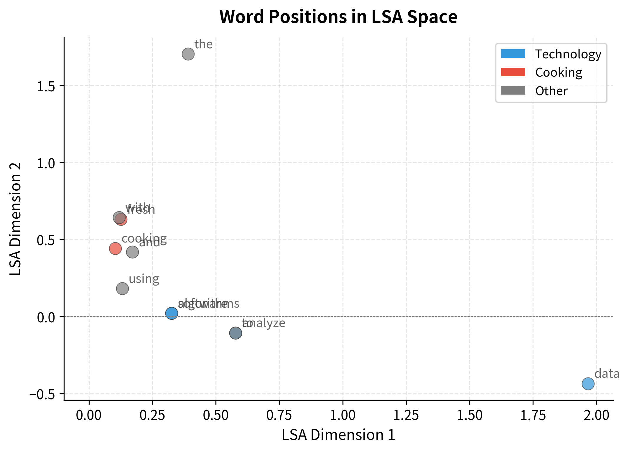
Visualizing the Semantic Space
The scatter plot below shows words positioned by their first two LSA coordinates. Even with just two dimensions, the semantic organization is visible.
Documents can also be visualized in the same LSA space, revealing how they cluster by topic.
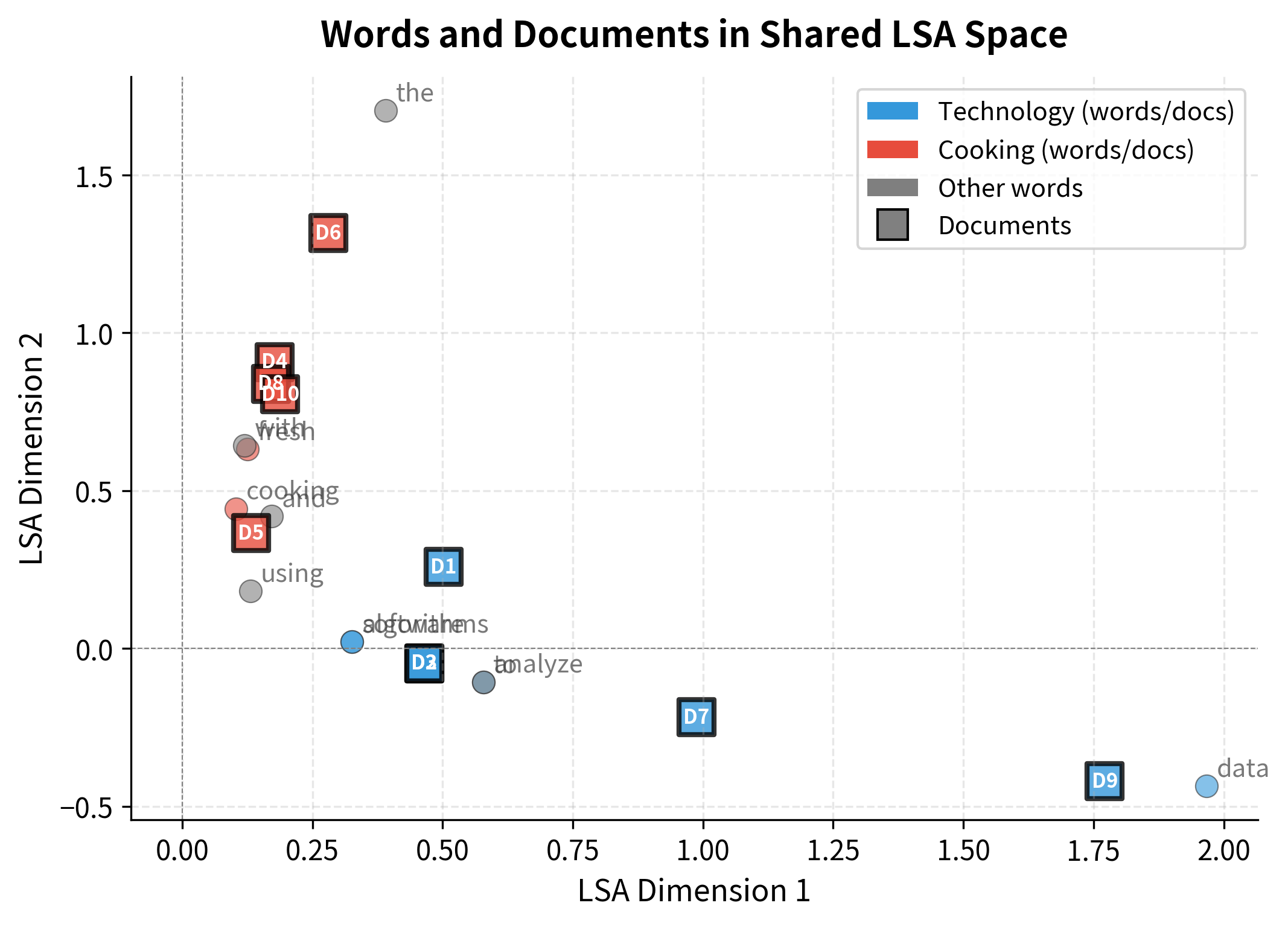
This joint visualization reveals a key property of LSA: words and documents live in the same semantic space. A document's position is essentially the weighted average of its words' positions. This shared representation enables powerful applications like finding documents similar to a query word, or finding words that characterize a document.
Computing Semantic Similarity
With words represented as dense vectors, computing similarity becomes straightforward and efficient. We use cosine similarity, the cosine of the angle between two vectors, which measures how aligned two words are in the semantic space, regardless of their vector magnitudes.
The results demonstrate LSA's power: words are similar based on meaning, not just co-occurrence. "Data" clusters with "algorithms" because they appear in similar documents, such as technology articles, programming tutorials, and data science content. "Cooking" clusters with "chef" and "kitchen" for the same reason.
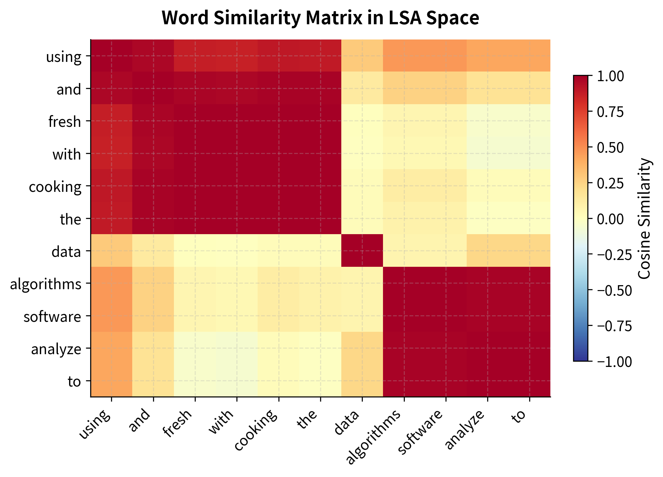
The similarity heatmap reveals the semantic structure LSA has discovered. Words are reordered using hierarchical clustering to group similar words together. The resulting block structure shows clear semantic clusters: technology terms cluster together, cooking terms form another block, with low similarity (cooler colors) between the domains.
The key insight: LSA discovers similarity through transitive relationships. Even if "data" and "algorithms" never appear in the same sentence, they're similar because they both appear with words like "computer," "software," and "analysis." The SVD compression captures these indirect relationships that raw co-occurrence counts miss.
Choosing the Number of Dimensions
We've seen that truncated SVD works, but we've glossed over a critical decision: how many dimensions should we keep?
This isn't just a technical detail. The choice of fundamentally affects what your model captures:
- Too few dimensions: You lose important distinctions. "Car" and "automobile" might be similar, but so might "car" and "truck" if you've collapsed too much structure.
- Too many dimensions: You keep noise. The model memorizes idiosyncratic patterns that don't generalize to new data.
The sweet spot depends on your data and your task. Here are the main approaches for finding it.
The Elbow Method: Visual Inspection
The simplest approach is to plot the singular values and look for an elbow, a point where the curve bends from steep decline to gradual decay. Dimensions before the elbow capture signal; those after capture noise.
Task-Based Selection: Let Performance Decide
The elbow method gives a starting point, but the best approach is often empirical: evaluate different dimension counts on your actual task.
- For document retrieval: Measure precision and recall at different values
- For word similarity: Compare against human similarity judgments (datasets like SimLex-999)
- For classification: Use cross-validation accuracy as your guide
The "optimal" varies by task. A word similarity task might need 300 dimensions to capture fine distinctions, while a topic classification task might work best with 50 dimensions that capture broad categories.
The reconstruction error drops rapidly with the first few dimensions, then levels off. This pattern of steep initial decline followed by diminishing returns is characteristic of structured data. The first dimensions capture the dominant patterns; additional dimensions add progressively less information, eventually just fitting noise.
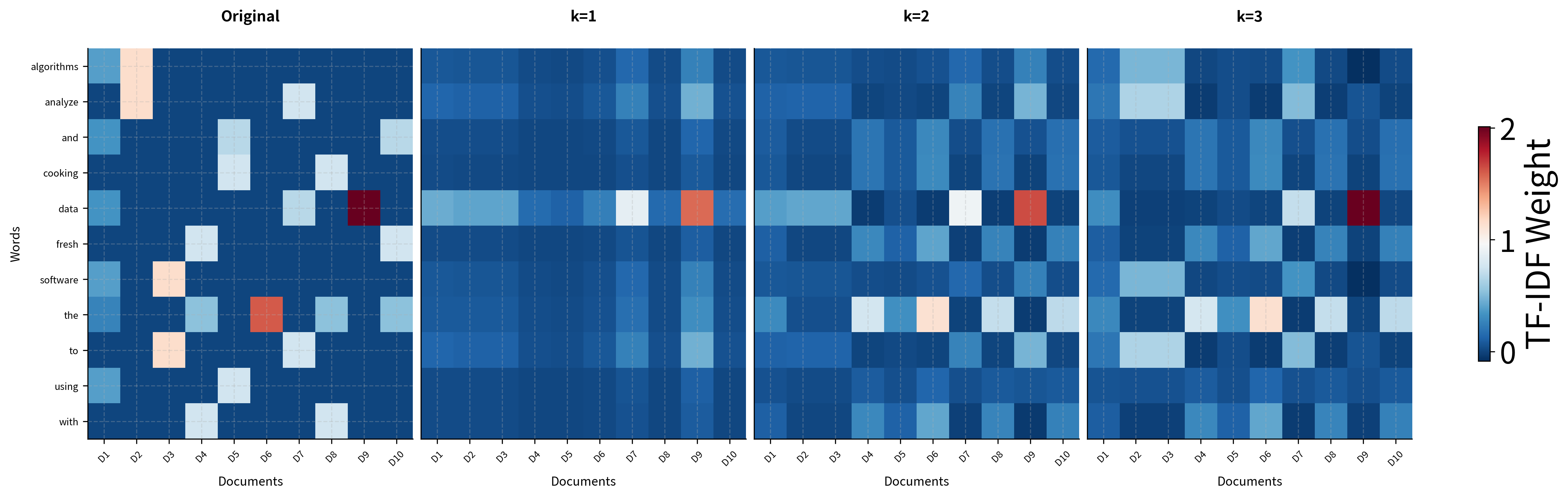
The progression from k=1 to k=3 shows how each additional dimension adds information. The rank-1 approximation captures only the most dominant pattern (overall word frequency). Rank-2 begins to distinguish between document types. By rank-3, the reconstruction closely matches the original, capturing the essential semantic structure while smoothing out idiosyncratic noise.
Practical Guidelines
For LSA on typical document collections:
- 50-300 dimensions is a common range for document retrieval and topic modeling
- 100-500 dimensions works well for word similarity tasks
- Start with 100 dimensions as a baseline and tune from there
- More data generally supports more dimensions without overfitting
Rule of thumb: Start with where is the number of documents, then tune based on task performance. For word-word matrices, between 100 and 500 typically works well.
Computational Complexity: The Scaling Challenge
Everything we've discussed works beautifully on small datasets. But real-world NLP deals with massive scale: vocabularies of 100,000+ words, corpora with millions of documents. Here, SVD's computational cost becomes a serious obstacle.
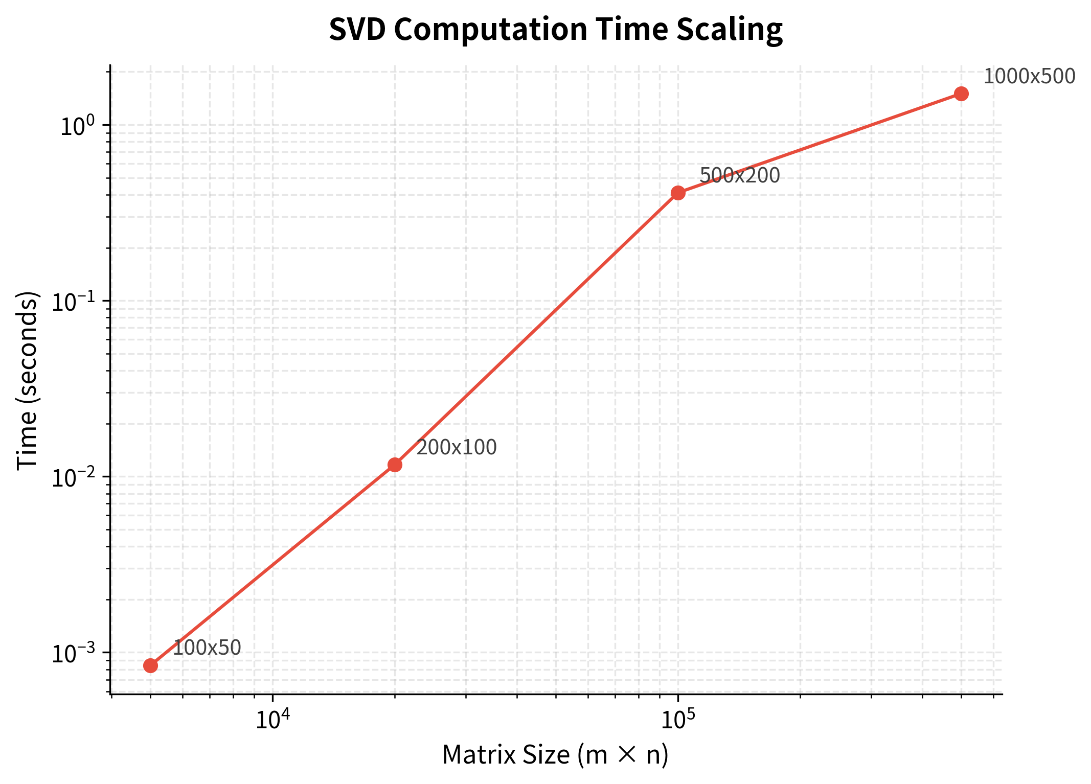
Full SVD has complexity , where is the number of rows (vocabulary size) and is the number of columns (documents or context words). This is roughly cubic in the matrix dimensions. For a 100,000 × 50,000 matrix, this means billions of operations. Even on fast hardware, computation takes hours or days.
Randomized SVD: Making Scale Tractable
The scaling problem seems insurmountable, until you realize we don't actually need the full SVD. We only want the top components, and we've seen that is typically small (50-500). Can we compute just those components without computing everything?
Randomized SVD answers yes, achieving complexity, where and are the matrix dimensions and is the number of components we want to keep. This is linear in the matrix size. For a 100,000 × 50,000 matrix with , this is 500× faster than full SVD.
The Key Insight: Random Projection
The algorithm rests on a beautiful idea: random projection preserves structure. If we multiply our matrix by a random matrix, we get a smaller matrix that captures most of the original's important directions. We can then compute SVD on this smaller matrix and recover an approximation to the original SVD.
Why does randomness help? Because the important directions (those with large singular values) are robust and show up even after random projection. The unimportant directions (small singular values) get scrambled, but we didn't want them anyway.
Comparing Randomized to Full SVD
Let's verify that randomized SVD delivers on its promise: comparable accuracy at a fraction of the cost.
The results confirm the theory: randomized SVD achieves nearly identical reconstruction error while running significantly faster. The small accuracy gap (typically 1-2%) is a worthwhile trade-off for the dramatic speedup.
Production Implementation: scikit-learn
For production use, scikit-learn's TruncatedSVD provides an optimized implementation with sensible defaults. It uses randomized algorithms automatically for large matrices.
Scikit-learn's implementation is fast, numerically stable, and handles edge cases gracefully. For most applications, this is the recommended approach. There's no need to implement randomized SVD yourself unless you have specialized requirements.
Interpreting SVD Dimensions
One of SVD's advantages over neural embeddings is interpretability. While the dimensions don't have predetermined meanings, we can often understand what they capture by examining which words load most strongly on each pole.
This interpretability has practical value: it helps us understand what our model has learned, diagnose problems, and explain results to stakeholders.
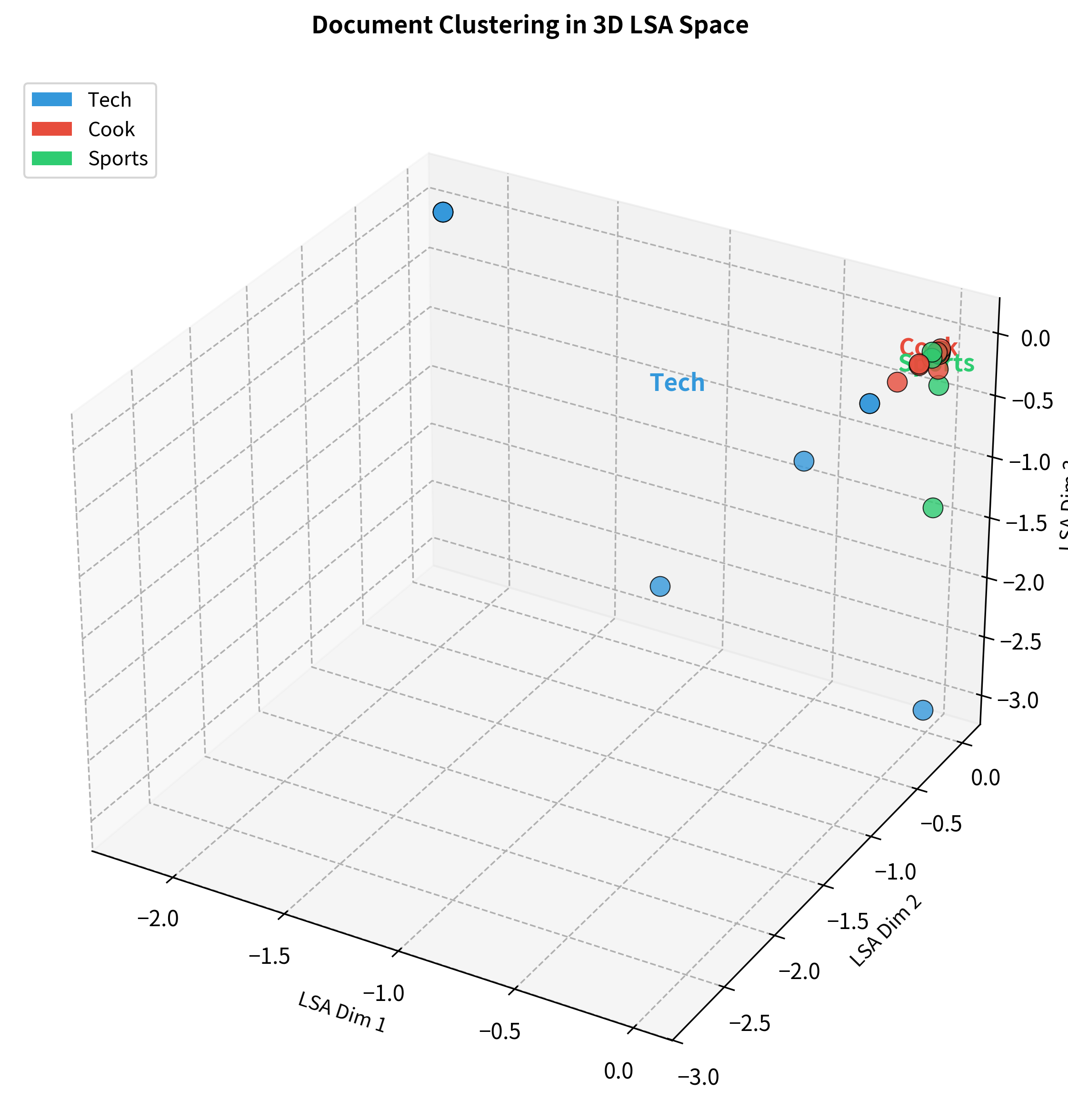
The 3D visualization shows how the three topic clusters separate in LSA space. Technology documents cluster in one region, cooking documents in another, and sports documents in a third. This clear separation emerges purely from analyzing word co-occurrence patterns. We never told the algorithm about these categories.
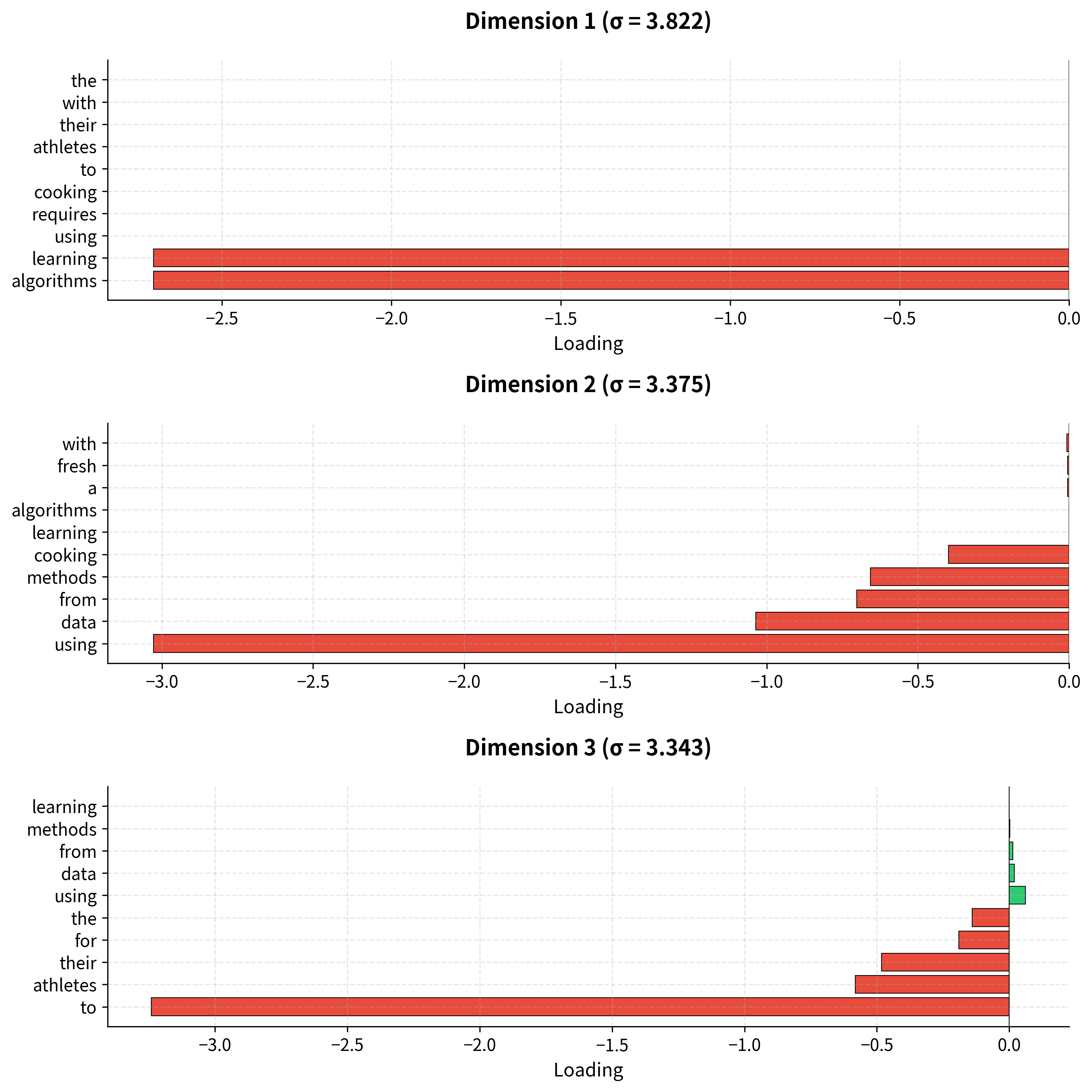
The bar charts reveal the semantic contrasts each dimension captures. The first dimension might separate technology from cooking; the second might capture a different contrast (perhaps abstract vs. concrete, or formal vs. informal). Later dimensions capture progressively subtler distinctions.
A note on interpretation: Not every dimension will have a clear human-interpretable meaning. Some capture complex combinations of features, or statistical patterns that don't map neatly to concepts. This is fine. The dimensions are optimized for reconstruction accuracy, not human interpretability.
SVD on Word-Word Matrices
So far we've applied SVD to term-document matrices, where similarity reflects shared document membership. But there's another approach: apply SVD to word-word co-occurrence matrices, where similarity reflects shared local context.
These two approaches capture different aspects of meaning:
- Term-document (LSA): Words are similar if they appear in similar documents → captures topical/thematic similarity
- Word-word (SVD on co-occurrence): Words are similar if they appear near similar words → captures syntactic and fine-grained semantic similarity
The word-word matrix is even sparser than the term-document matrix. Most word pairs never appear within a few words of each other. This extreme sparsity makes dimensionality reduction essential: the raw co-occurrence counts are too noisy and sparse for reliable similarity computation.
PPMI Transformation: Better Than Raw Counts
Before applying SVD, we transform the co-occurrence counts using Positive Pointwise Mutual Information (PPMI). This transformation converts raw counts into association scores that better reflect semantic relationships.
The intuition: raw counts overweight frequent words. "The" co-occurs with everything, but this tells us nothing about meaning. PPMI asks: "Does this word pair co-occur more than we'd expect by chance?" High PPMI indicates a meaningful association; low PPMI indicates coincidental co-occurrence.
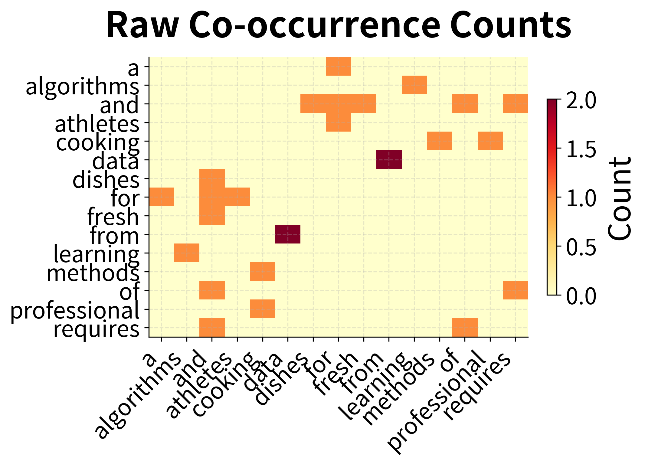
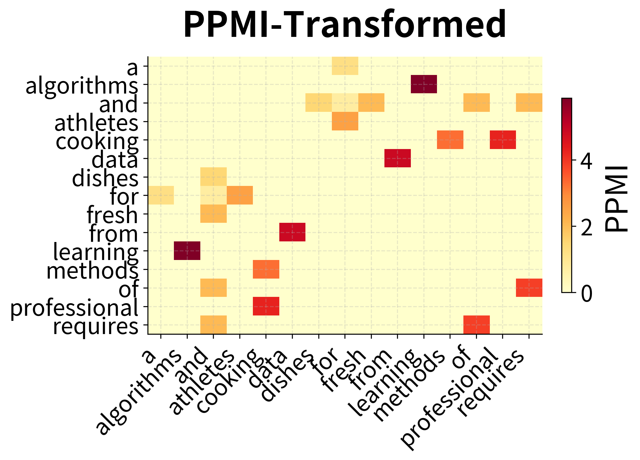
The comparison reveals PPMI's effect: raw counts show high values wherever frequent words appear, regardless of semantic meaning. PPMI normalizes for frequency, highlighting word pairs that co-occur more than expected by chance. These are the meaningful semantic associations.
Compare these results to the term-document LSA similarities earlier. The word-word approach captures different relationships, focusing more on syntactic and local semantic patterns, less on broad topical similarity.
Which approach is better? It depends on your task:
- For document retrieval and topic modeling: Term-document LSA captures the relevant structure
- For word similarity and analogy tasks: Word-word SVD often performs better
- For general-purpose embeddings: Word-word approaches (which inspired Word2Vec and GloVe) have become the standard
Limitations of SVD-Based Methods
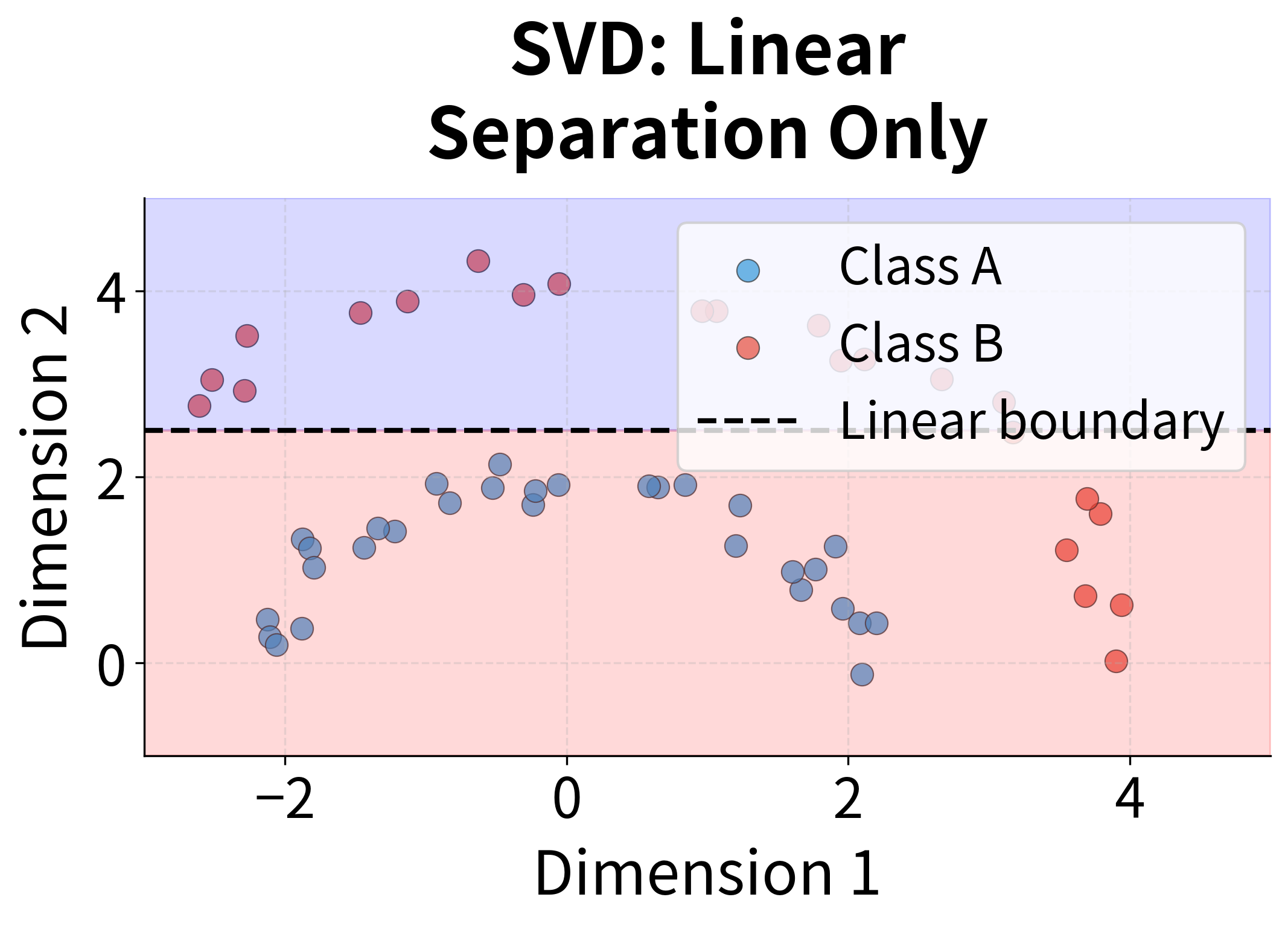
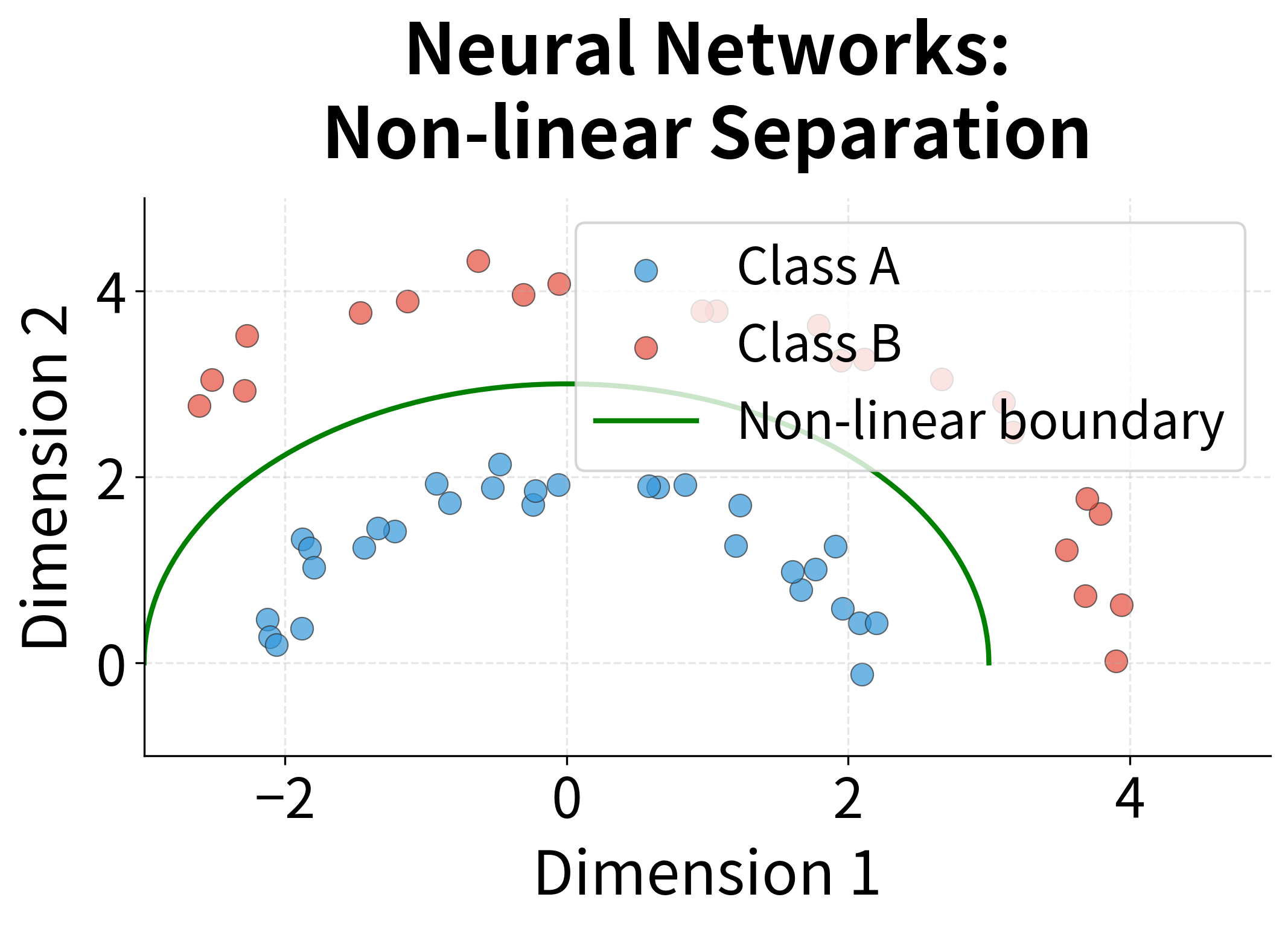
While powerful, SVD has limitations that motivated the development of neural word embeddings:
- Linear assumption: SVD finds linear combinations of the original dimensions. It cannot capture non-linear relationships in the data.
- Static representations: Each word gets a single vector regardless of context. "Bank" (financial) and "bank" (river) have the same representation.
- Scalability: Even with randomized algorithms, SVD struggles with web-scale corpora containing billions of words.
- Incremental updates: Adding new documents requires recomputing the entire decomposition. There's no efficient way to update the model incrementally.
- Out-of-vocabulary words: Words not seen during training have no representation.
Historical Impact and Modern Relevance
Despite its limitations, SVD-based methods had enormous impact on NLP:
- Information retrieval: LSA revolutionized document search by enabling semantic matching. Queries could find relevant documents even without exact keyword overlap.
- Dimensionality reduction: The principle of finding low-rank approximations influenced all subsequent embedding methods, including Word2Vec and GloVe.
- Interpretability: SVD dimensions often correspond to interpretable concepts, unlike the opaque representations of deep neural networks.
- Theoretical foundation: SVD provides optimality guarantees that neural methods lack. The Eckart-Young theorem ensures we're finding the best possible low-rank approximation.
Modern neural embeddings like Word2Vec can be understood as implicit matrix factorization. Levy and Goldberg (2014) showed that skip-gram with negative sampling implicitly factorizes a shifted PMI matrix, connecting neural methods back to the SVD tradition.
Summary
Singular Value Decomposition transforms sparse, high-dimensional co-occurrence data into dense, low-dimensional representations that capture semantic structure.
Key concepts:
- SVD factorization decomposes a matrix into , where and are orthogonal matrices and contains singular values
- Truncated SVD keeps only the top dimensions, providing the optimal rank- approximation
- Singular values indicate dimension importance; their decay reveals the data's intrinsic dimensionality
- LSA applies SVD to term-document matrices to discover latent semantic structure
- Randomized SVD enables scaling to large matrices with complexity
Practical considerations:
- Choose dimensions using the elbow method or task-based evaluation
- Apply TF-IDF or PPMI weighting before SVD for better results
- Use randomized algorithms (like scikit-learn's TruncatedSVD) for large matrices
- Interpret dimensions by examining top-loading words on each pole
Limitations:
- Linear method cannot capture non-linear relationships
- Static representations don't handle polysemy
- Requires recomputation for new documents
- No representation for out-of-vocabulary words
SVD-based methods remain relevant as baselines and for interpretability. Understanding them provides essential background for the neural embedding methods that followed, which we'll explore in subsequent chapters.
Key Parameters
When applying SVD to text data, these parameters have the greatest impact on the quality and utility of the resulting representations:
| Parameter | Typical Range | Effect |
|---|---|---|
n_components | 50-500 | Number of dimensions to retain. More components capture more variance but increase computation and may include noise. |
algorithm | 'arpack', 'randomized' | 'randomized' is faster for large matrices; 'arpack' is more precise for small matrices. |
n_iter | 2-10 | Power iterations for randomized SVD. More iterations improve accuracy at the cost of speed. |
n_oversamples | 10-20 | Extra dimensions sampled in randomized SVD. Improves approximation quality with minimal overhead. |
Choosing n_components:
- For document retrieval and topic modeling: 50-300 dimensions typically work well
- For word similarity tasks: 100-500 dimensions capture finer distinctions
- Use the elbow method on singular value decay to identify where signal ends and noise begins
- When in doubt, start with 100 and tune based on downstream task performance
Preprocessing choices:
- TF-IDF weighting: Almost always beneficial for term-document matrices. Down-weights frequent terms that appear everywhere.
- PPMI transformation: Recommended for word-word matrices. Converts raw counts to association scores.
- Centering: Optional. Mean-centering rows or columns can improve results for some tasks.
Computational considerations:
- For matrices larger than 10,000 x 10,000, use randomized SVD (
algorithm='randomized') - Sparse matrix formats (CSR, CSC) reduce memory requirements significantly
- Consider incremental/online variants if data arrives in streams
Quiz
Ready to test your understanding? Take this quick quiz to reinforce what you've learned about Singular Value Decomposition and Latent Semantic Analysis.

Comments