

Learn how Pointwise Mutual Information (PMI) transforms raw co-occurrence counts into meaningful word association scores by comparing observed frequencies to expected frequencies under independence.

This article is part of the free-to-read Language AI Handbook
Choose your expertise level to adjust how many terms are explained. Beginners see more tooltips, experts see fewer to maintain reading flow. Hover over underlined terms for instant definitions.
Pointwise Mutual Information
Raw co-occurrence counts tell us how often words appear together, but they have a fundamental problem: frequent words dominate everything. The word "the" co-occurs with nearly every other word, not because it has a special relationship with them, but simply because it appears everywhere. How do we separate meaningful associations from mere frequency effects?
Pointwise Mutual Information (PMI) solves this problem by asking a different question: does this word pair co-occur more than we'd expect by chance? Instead of counting raw co-occurrences, PMI measures the surprise of seeing two words together. When "New" and "York" appear together far more often than their individual frequencies would predict, PMI captures that strong association. When "the" and "dog" appear together only as often as expected, PMI correctly identifies this as an unremarkable pairing.
This chapter derives the PMI formula from probability theory, shows how it transforms co-occurrence matrices into more meaningful representations, and demonstrates its practical applications from collocation extraction to improved word vectors.
The Problem with Raw Counts
Let's start by understanding why raw co-occurrence counts are problematic. Consider a corpus about animals and food:
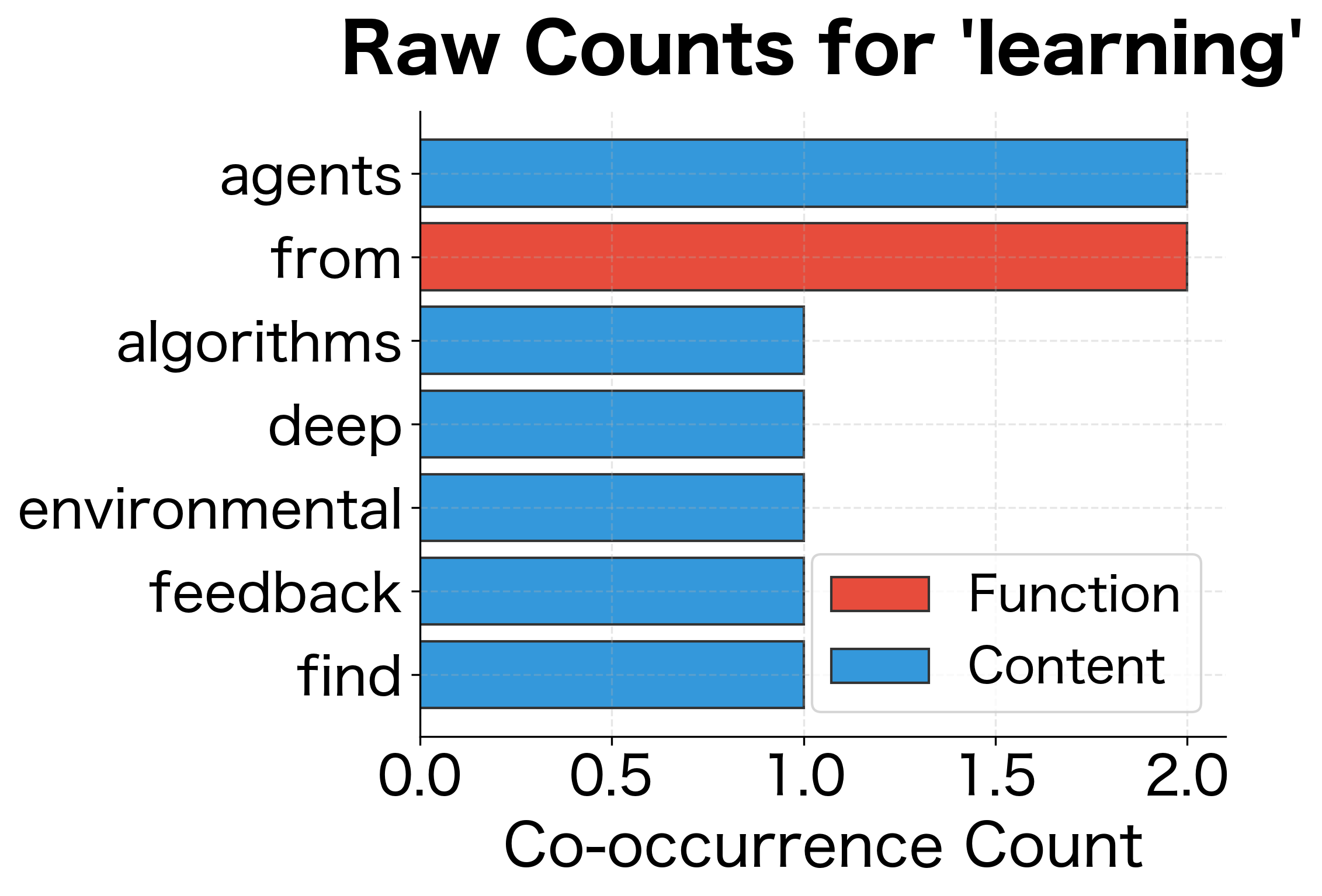
The word "the" appears 18 times, dwarfing content words like "cat" (5 times) or "new" (3 times). In a raw co-occurrence matrix, "the" will have high counts with almost everything, obscuring the meaningful associations we care about.
The raw counts show "the" as the top co-occurrence for "cat," but this tells us nothing about cats. The word "the" appears near everything. We need a measure that accounts for how often we'd expect words to co-occur given their individual frequencies.
The PMI Formula
The problem we identified, that frequent words dominate co-occurrence counts, stems from a fundamental issue: raw counts conflate two distinct phenomena. When "the" appears near "cat" 10 times, is that because "the" and "cat" have a special relationship, or simply because "the" appears near everything 10 times? To separate genuine associations from frequency effects, we need to ask a different question: how does the observed co-occurrence compare to what we'd expect if the words were unrelated?
Pointwise Mutual Information answers this question directly. Instead of asking "how often do these words appear together?" PMI asks "do these words appear together more or less than chance would predict?"
The Intuition: Observed vs Expected
Consider two words, and . If they have no special relationship, their co-occurrence should follow a simple pattern: the probability of seeing them together should equal the product of their individual probabilities. This is the definition of statistical independence.
For example, if "cat" appears in 5% of contexts and "mouse" appears in 2% of contexts, and they're independent, we'd expect "cat" and "mouse" to co-occur in roughly of word pairs. If they actually co-occur in 1% of pairs, that's 10 times more than expected. This excess reveals a genuine association.
PMI formalizes this comparison by taking the ratio of observed to expected co-occurrence:
where:
- : the target word whose associations we want to measure
- : the context word that may or may not be associated with
- : the joint probability of observing and together in the same context window
- : the marginal probability of word appearing in any context
- : the marginal probability of word appearing in any context
- : the expected joint probability if and were statistically independent
- : the base-2 logarithm, which converts ratios to bits of information
PMI measures the association between two words by comparing their joint probability of co-occurrence to what we'd expect if they were independent. High PMI indicates the words are strongly associated; low or negative PMI indicates they co-occur less than expected by chance.
Let's unpack each component of this formula:
-
Numerator : The joint probability, measuring how often words and actually co-occur in the corpus. This is the observed co-occurrence rate.
-
Denominator : The expected probability under independence. If the words were unrelated, this is how often they would co-occur by chance. This follows from the definition of statistical independence: two events and are independent if and only if .
-
The ratio : When observed equals expected, the ratio is 1. When observed exceeds expected, the ratio is greater than 1. When observed falls short of expected, the ratio is less than 1.
-
The logarithm: Taking converts multiplicative relationships to additive ones. A ratio of 2 (twice as often as expected) becomes PMI of 1. A ratio of 4 becomes PMI of 2. This logarithmic scale makes PMI values easier to interpret and compare.
Why the Logarithm?
The logarithm serves three important purposes in the PMI formula.
1. Converting ratios to differences (additive scale)
Without the logarithm, we'd be working with a ratio that has an asymmetric range: values above 1 indicate positive association, while values between 0 and 1 indicate negative association. The logarithm maps this to a symmetric scale:
| Ratio (observed/expected) | PMI ( of ratio) |
|---|---|
| 8× | +3 |
| 4× | +2 |
| 2× | +1 |
| 1× (independence) | 0 |
| 0.5× | −1 |
| 0.25× | −2 |
| 0.125× | −3 |
The additive scale is more intuitive: PMI of 2 means "4 times more than expected," while PMI of 1 means "2 times more." Each unit of PMI represents a doubling.
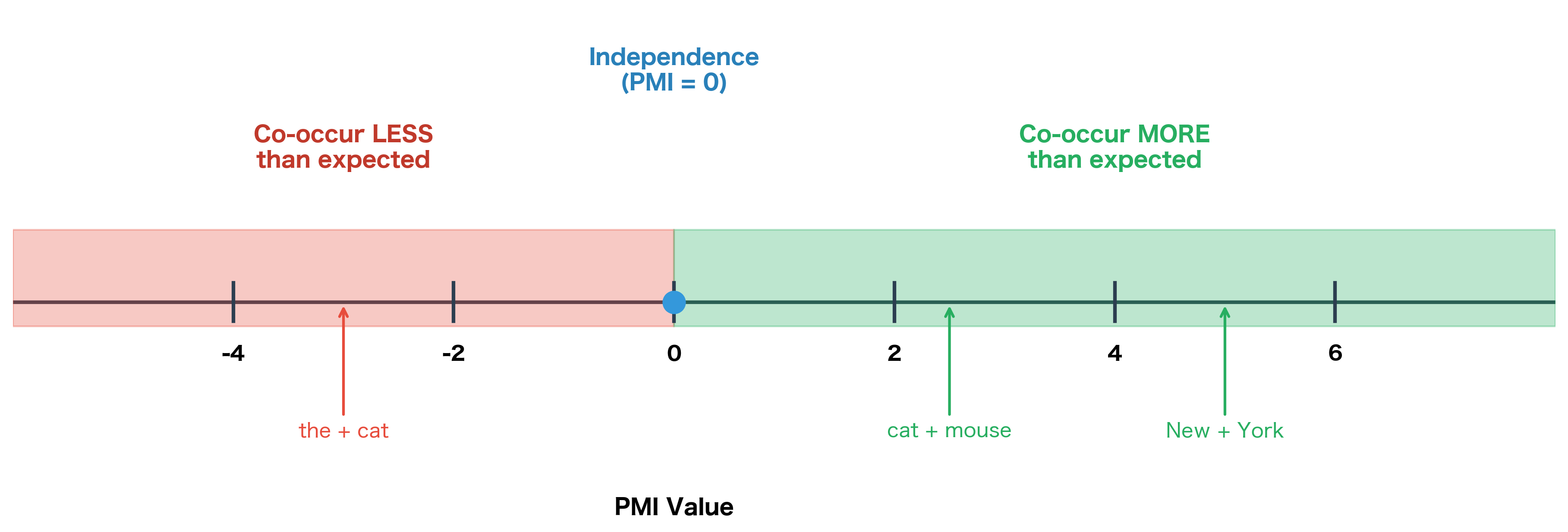
2. Creating symmetry around zero
Positive PMI indicates attraction (words co-occur more than expected), negative PMI indicates repulsion (words co-occur less than expected), and zero indicates independence. This symmetry makes it easy to compare and rank associations.
3. Connection to information theory
PMI measures how much information (in bits, when using ) observing one word provides about the other. In information-theoretic terms, PMI quantifies the reduction in uncertainty about word when we observe word . When two words are strongly associated, seeing one tells you a lot about whether you'll see the other.
From Probabilities to Counts
In practice, we don't know the true probabilities. We estimate them from corpus counts using the maximum likelihood principle: the best estimate of a probability is the observed frequency. Let denote how many times words and co-occur within the same context window, and let be the total number of word-context pairs in our co-occurrence matrix.
The probability estimates follow naturally from frequency ratios:
Joint probability (how often and appear together):
where:
- : the count of times words and co-occur within a context window
- : the total number of word-context pairs (sum of all entries in the co-occurrence matrix)
This is the fraction of all word pairs that are specifically the pair.
Marginal probability of the target word (how often appears with any context):
where:
- : the sum of co-occurrence counts across all context words
- : a shorthand notation meaning "sum over all context words"
This is the fraction of all pairs where the target word is . In the co-occurrence matrix, this equals the row sum for word .
Marginal probability of the context word (how often appears as context for any word):
where:
- : the sum of co-occurrence counts across all target words
- : a shorthand notation meaning "sum over all target words"
This equals the column sum for context word in the co-occurrence matrix.
The Practical Formula
Substituting these probability estimates into the PMI formula, we can derive a count-based version that's easier to compute directly from the co-occurrence matrix.
Step 1: Start with the definition and substitute our probability estimates:
Step 2: Simplify the denominator by multiplying the two fractions:
Step 3: Dividing by a fraction is equivalent to multiplying by its reciprocal:
Step 4: Cancel one factor of from numerator and denominator:
This is the formula we implement: multiply the co-occurrence count by the total, divide by the product of marginals, and take the logarithm.
where:
- : how often and actually co-occur (the observed count)
- : total co-occurrences in the matrix (sum of all entries)
- : how often appears with any context (row sum for word )
- : how often appears as context for any word (column sum for context )
The product represents the expected count under independence: if word appears in a fraction of all pairs, and context appears in a fraction of all pairs, then under independence they should co-occur in approximately pairs.
Implementing PMI
Let's translate this formula into code. The implementation follows the mathematical derivation closely, computing each component step by step.
The key insight in this implementation is computing the expected counts efficiently. Rather than looping through all word pairs, we use matrix multiplication: row_sums @ col_sums produces an outer product where each cell contains . Dividing by gives us the expected count for each pair.
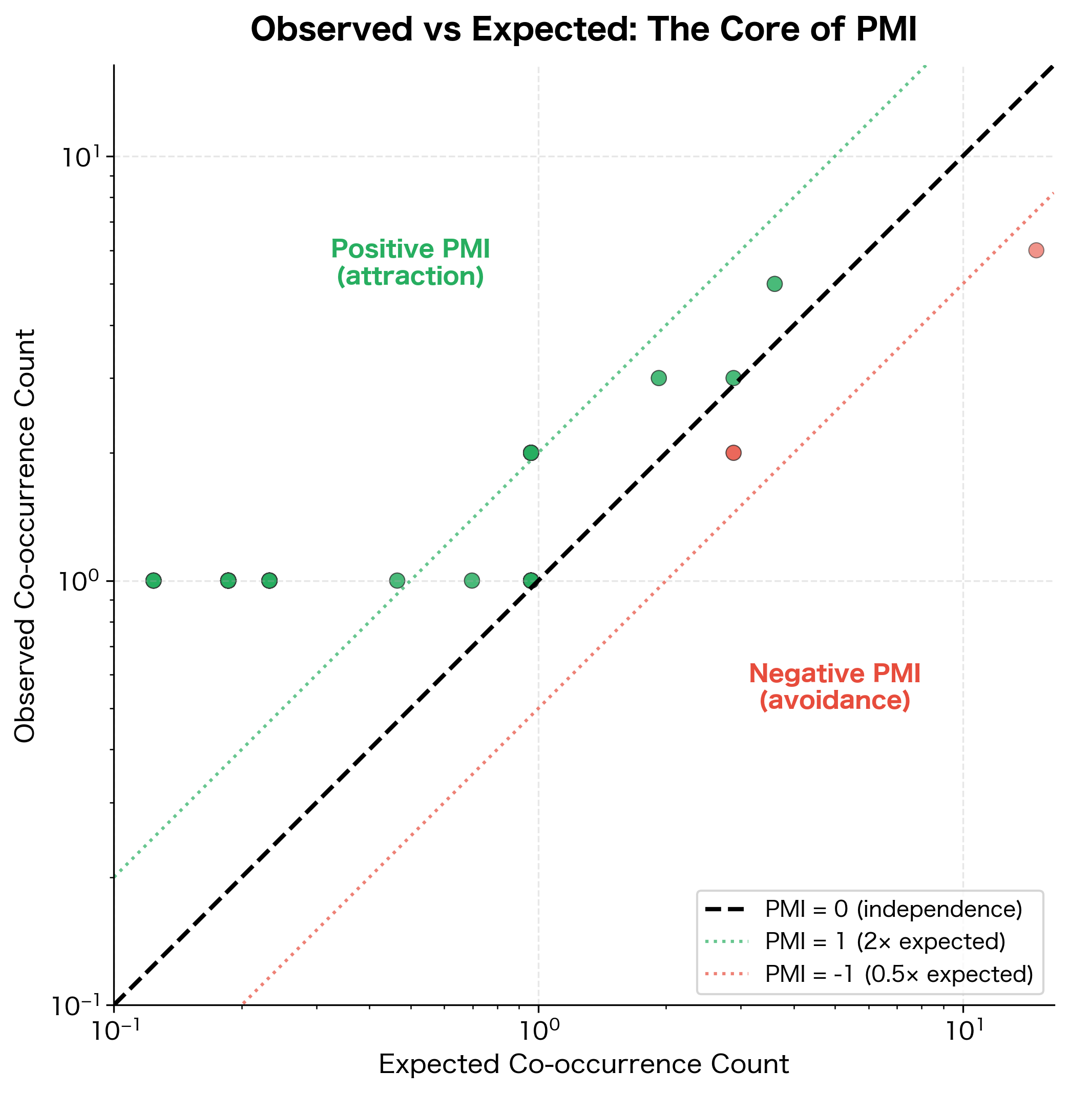
This scatter plot visualizes the fundamental idea behind PMI: comparing what we observe to what we'd expect. Word pairs above the diagonal have positive PMI (they co-occur more than chance predicts), while pairs below have negative PMI.
The transformation is dramatic. Raw counts ranked "the" as the top co-occurrence for "cat," but PMI reveals a different picture. Words that specifically associate with "cat," rather than appearing everywhere, now rise to the top. The word "the" has low or negative PMI because its high frequency means it co-occurs with "cat" about as often as we'd expect by chance.
Interpreting PMI as Association Strength
The logarithmic scale of PMI creates a natural interpretation centered on zero. Because we're measuring , the value tells us directly how the actual co-occurrence compares to the baseline of independence.
The key insight is that PMI values correspond to powers of 2. If , then:
This means the observed probability equals times the expected probability under independence. Conversely, we can convert a ratio of observed to expected into PMI via .
-
PMI > 0: The words co-occur more than expected. A PMI of 1 means times as often as chance; PMI of 2 means times as often; PMI of 3 means times. The higher the value, the stronger the positive association.
-
PMI = 0: The words co-occur exactly as expected under independence (, so observed equals expected). There's no special relationship, either attractive or repulsive.
-
PMI < 0: The words co-occur less than expected. They tend to avoid each other. A PMI of -1 means times as often as chance would predict (i.e., half as often).
A Worked Example: Computing PMI Step by Step
To solidify understanding, let's walk through a complete PMI calculation by hand. We'll compute the PMI between "cat" and "mouse," two words we'd expect to have a strong association.
The calculation proceeds in three stages:
- Gather the raw counts from our co-occurrence matrix
- Compute the expected count under the assumption of independence
- Calculate PMI as the log ratio of observed to expected
The positive PMI confirms our linguistic intuition: "cat" and "mouse" have a genuine association in language. They appear together in contexts about predator-prey relationships, children's stories, and idiomatic expressions far more often than their individual frequencies would suggest.
This is exactly the kind of meaningful relationship PMI is designed to uncover. Raw counts would have told us that "the" co-occurs with "cat" more often than "mouse" does, simply because "the" is everywhere. PMI cuts through this noise by asking the right question: not "how often?" but "how much more than expected?"
The Problem with Negative PMI
While PMI can be negative (indicating words that avoid each other), negative values cause practical problems. Most word pairs never co-occur at all, giving them PMI of negative infinity. Even pairs that co-occur rarely get large negative values.
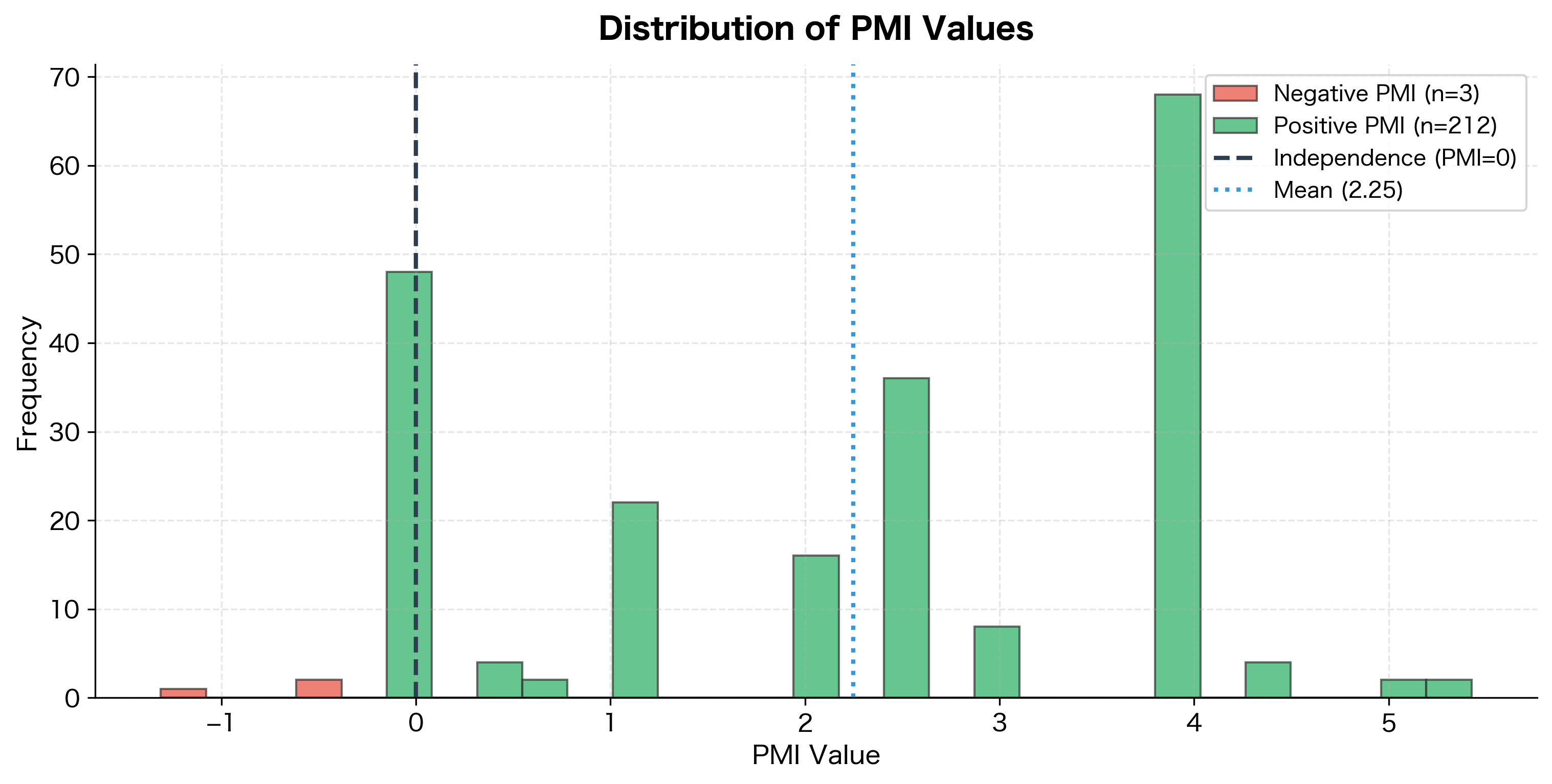
The histogram reveals a key characteristic of PMI: many word pairs have negative values, meaning they co-occur less than expected. This asymmetry, combined with the issues below, motivates the PPMI transformation.
Negative PMI values are problematic for several reasons:
-
Unreliable estimates: Low co-occurrence counts produce noisy PMI values. A word pair that co-occurs once when we expected two has PMI of -1, but this could easily be sampling noise.
-
Asymmetric information: Knowing that words don't co-occur is less informative than knowing they do. The absence of co-occurrence could mean many things.
-
Computational issues: Large negative values dominate distance calculations and can destabilize downstream algorithms.
Positive PMI (PPMI)
The standard solution is Positive PMI (PPMI), which simply clips negative values to zero:
where:
- : the pointwise mutual information between words and , as defined earlier
- : the maximum of 0 and , which returns if and returns 0 otherwise
The function effectively acts as a threshold: any word pair with negative PMI (indicating the words co-occur less than expected) is set to zero, while positive associations are preserved unchanged.
PPMI retains only the positive associations from PMI, treating all negative or zero associations as equally uninformative. This produces sparse, non-negative matrices that work well with many machine learning algorithms.
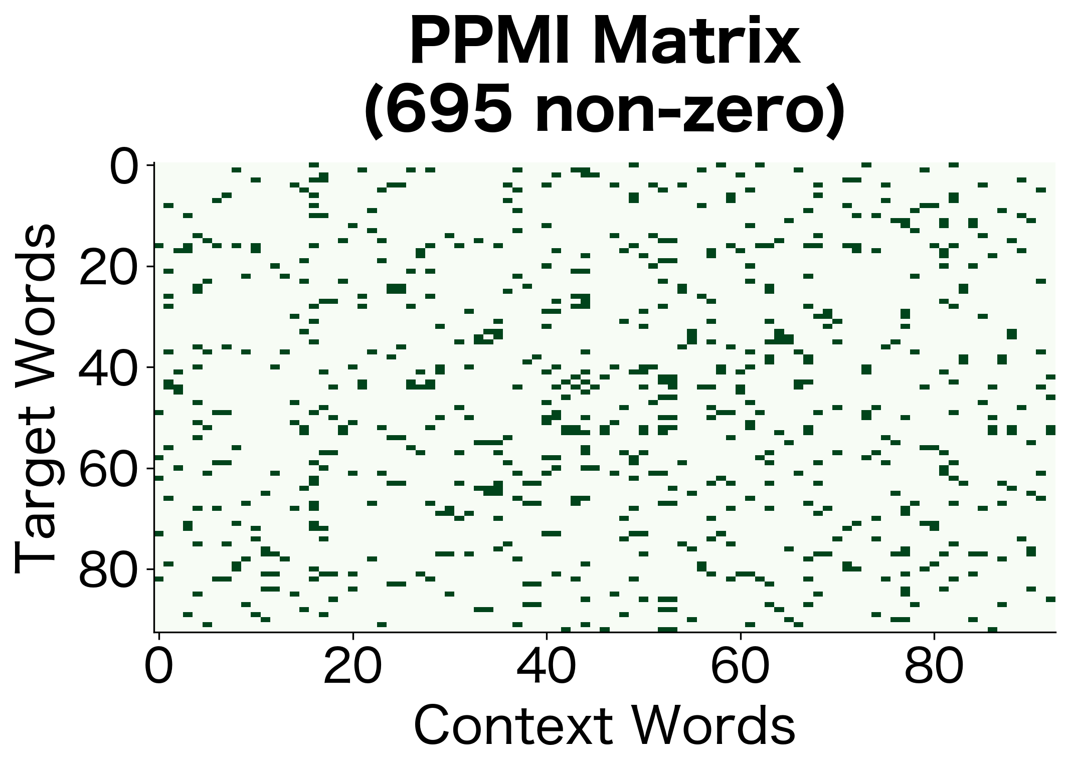
The high sparsity indicates that PPMI has filtered out most word pairs, retaining only those with genuine positive associations. The remaining non-zero entries represent meaningful relationships that exceed what independence would predict.
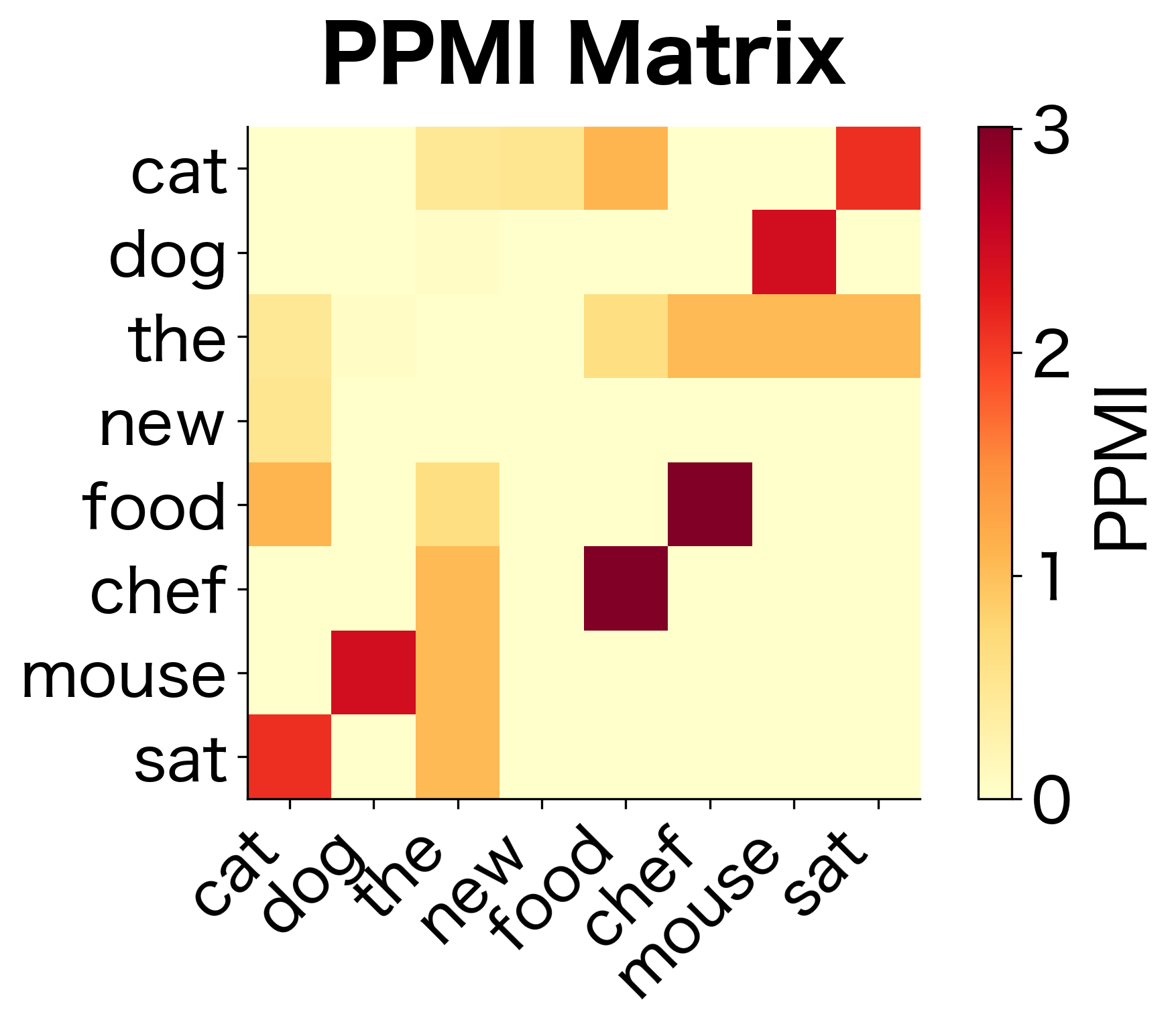
The PPMI matrix is much sparser than the raw co-occurrence matrix. Only word pairs with genuine positive associations retain non-zero values. This sparsity is a feature, not a bug: it means we've filtered out the noise of random co-occurrences.
Shifted PPMI Variants
While PPMI works well, researchers have developed variants that address specific issues. The most important is Shifted PPMI, which subtracts a constant before clipping:
where:
- : the pointwise mutual information between words and
- : the shift parameter, a positive integer typically between 1 and 15
- : the shift amount in bits (e.g., bits for )
The shift effectively raises the threshold for what counts as a "meaningful" association. To understand why, consider what the shift means mathematically:
- With : The shift is , so SPPMI equals standard PPMI. Any positive PMI is retained.
- With : The shift is . Only word pairs with PMI > 1 (co-occurring at least twice as often as expected) are retained.
- With : The shift is . Only word pairs that co-occur at least 5 times more than expected survive.
Shifted PPMI raises the bar for what counts as a positive association by subtracting before clipping. This filters out weak associations that might be due to noise, keeping only the strongest signals. Higher values produce sparser, more selective matrices.
The results show the filtering effect of higher values. As increases from 1 to 5, the number of retained associations drops substantially. This represents a trade-off: higher values filter out weaker (potentially noisy) associations but may also discard some genuine relationships.
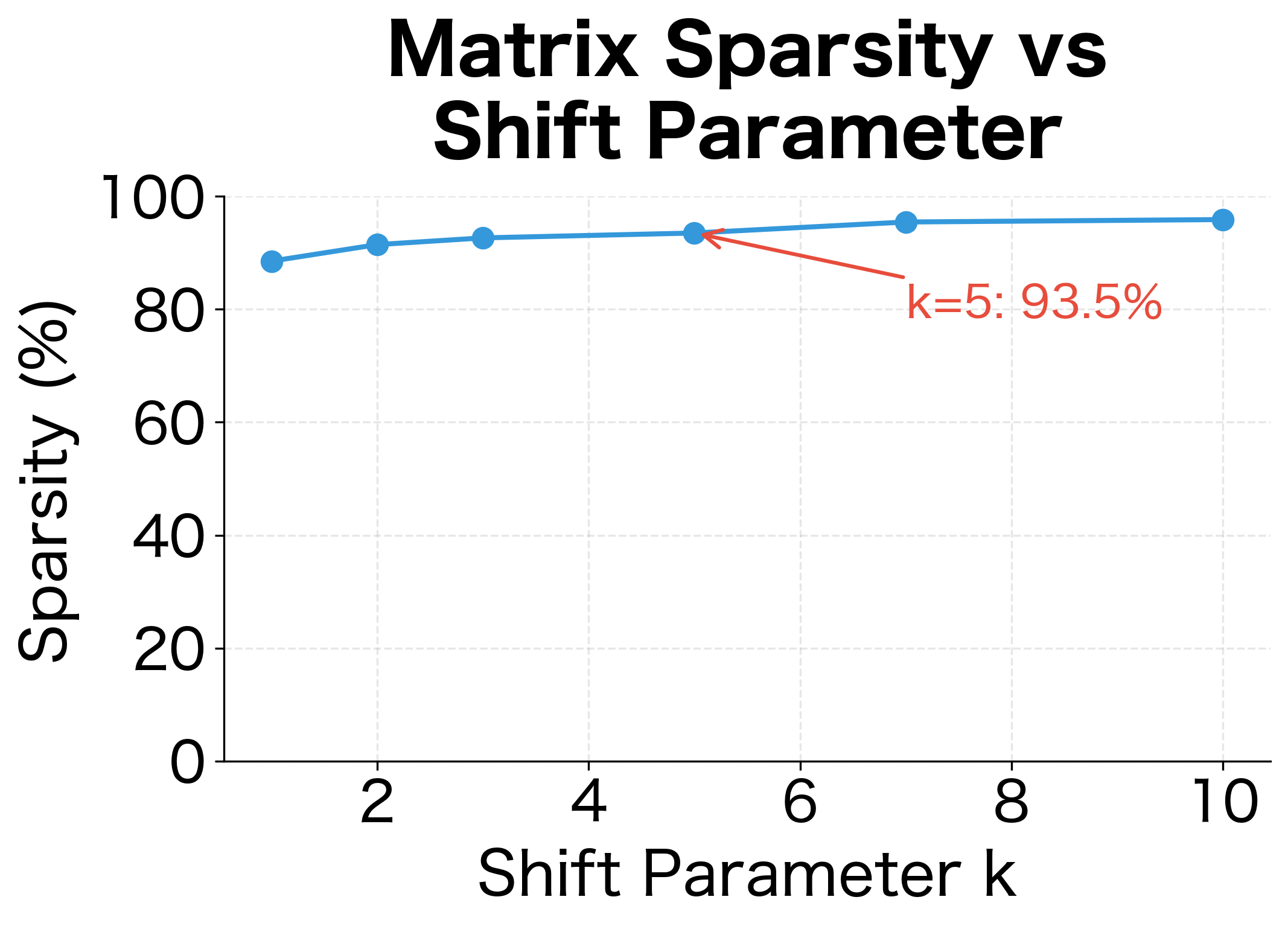
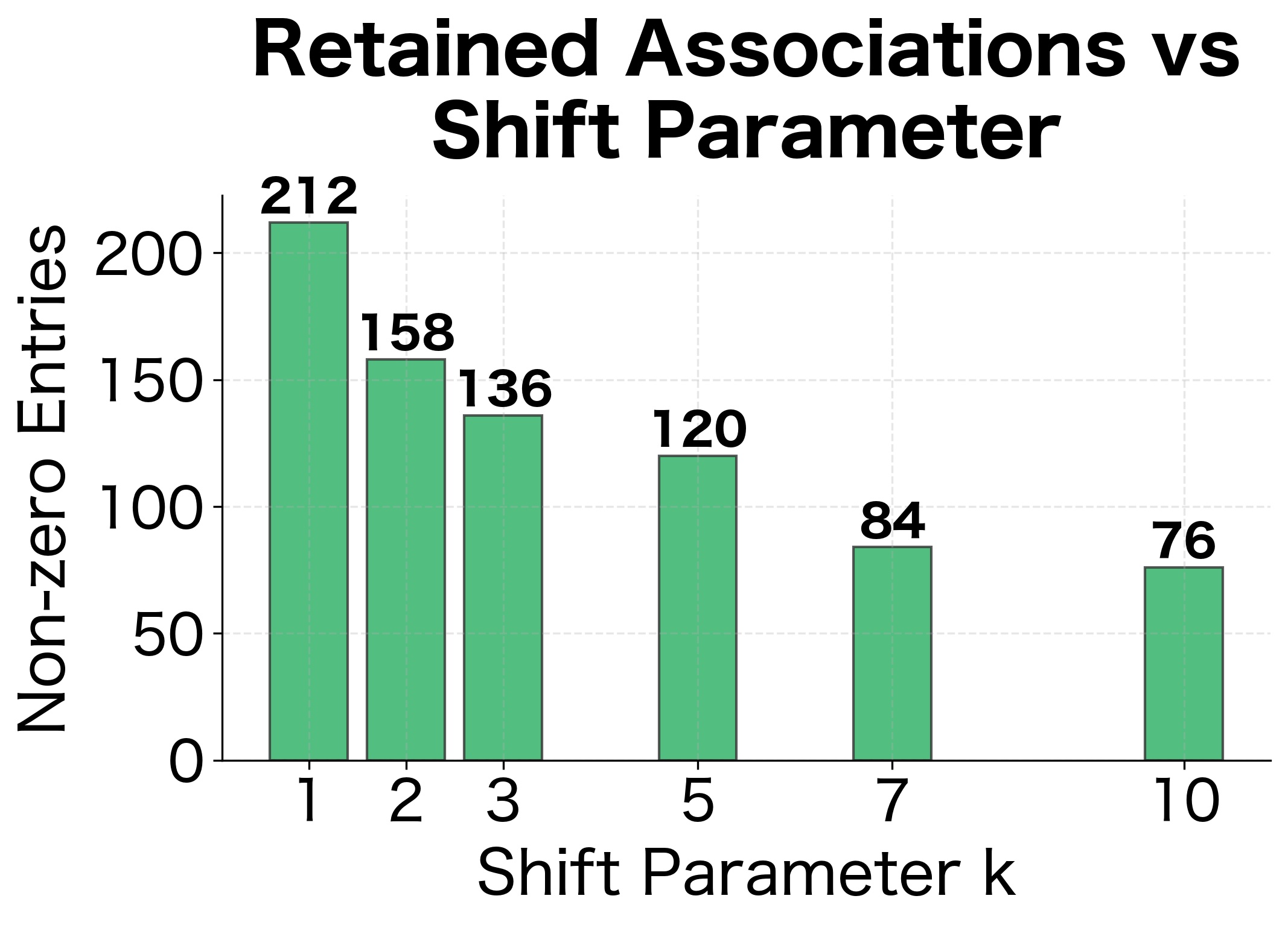
The visualization shows the trade-off clearly: higher shift values produce sparser matrices by filtering out weaker associations. A common choice is , which corresponds to Word2Vec's default of 5 negative samples.
The connection to Word2Vec is notable: Levy and Goldberg (2014) showed that Word2Vec's skip-gram model with negative sampling implicitly factorizes a shifted PMI matrix with equal to the number of negative samples. This theoretical connection explains why PMI-based methods and neural embeddings often produce similar results.
PMI vs Raw Counts: A Comparison
Let's directly compare how raw counts and PPMI rank word associations. We'll use a larger corpus to see clearer patterns.
The PPMI rankings are more semantically meaningful. Raw counts are dominated by frequent function words, while PPMI surfaces content words with genuine topical associations.
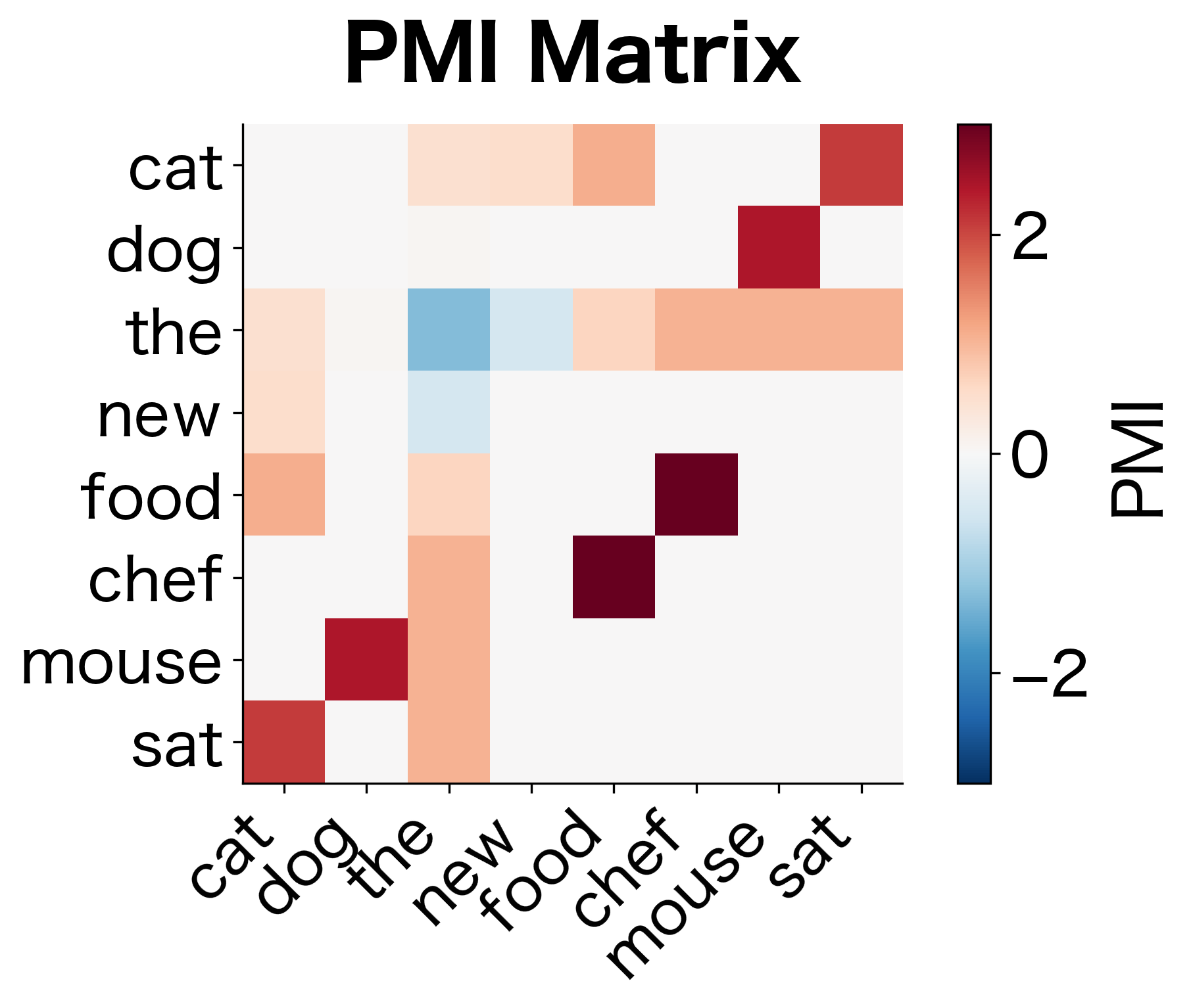
PMI Matrix Properties
PPMI matrices have several useful properties that make them well-suited for downstream NLP tasks.
Sparsity
PPMI matrices are highly sparse because most word pairs don't have positive associations. This sparsity enables efficient storage and computation.
The comparison reveals how PPMI filtering dramatically reduces the number of non-zero entries while increasing sparsity. This transformation discards pairs that co-occur at or below expected rates, retaining only the semantically meaningful associations.
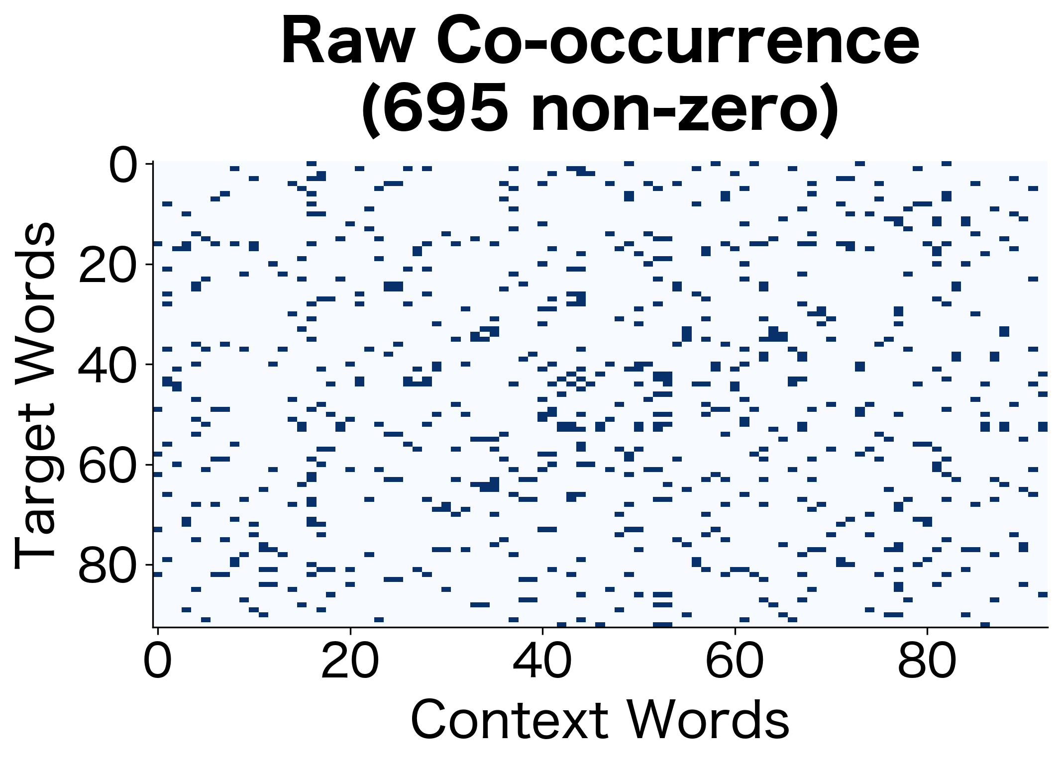
The sparsity visualization makes the filtering effect of PPMI immediately apparent. The raw matrix has entries wherever words co-occur at all, while the PPMI matrix retains only the genuinely positive associations. This much smaller subset captures the meaningful relationships.
Symmetry
For symmetric context windows (looking the same distance left and right), the co-occurrence matrix is symmetric, and so is the PPMI matrix: .
The matrix confirms symmetry, which means the association between words is bidirectional: if "neural" has high PPMI with "networks," then "networks" has equally high PPMI with "neural." This property holds when using symmetric context windows (looking the same distance left and right from each word).
Row Vectors as Word Representations
Each row of the PPMI matrix can serve as a word vector. Words with similar PPMI profiles (similar rows) tend to have similar meanings.
The similarity scores capture semantic relationships learned purely from co-occurrence patterns. Words appearing in similar contexts cluster together in the PPMI vector space, enabling applications like finding related terms or detecting semantic categories.
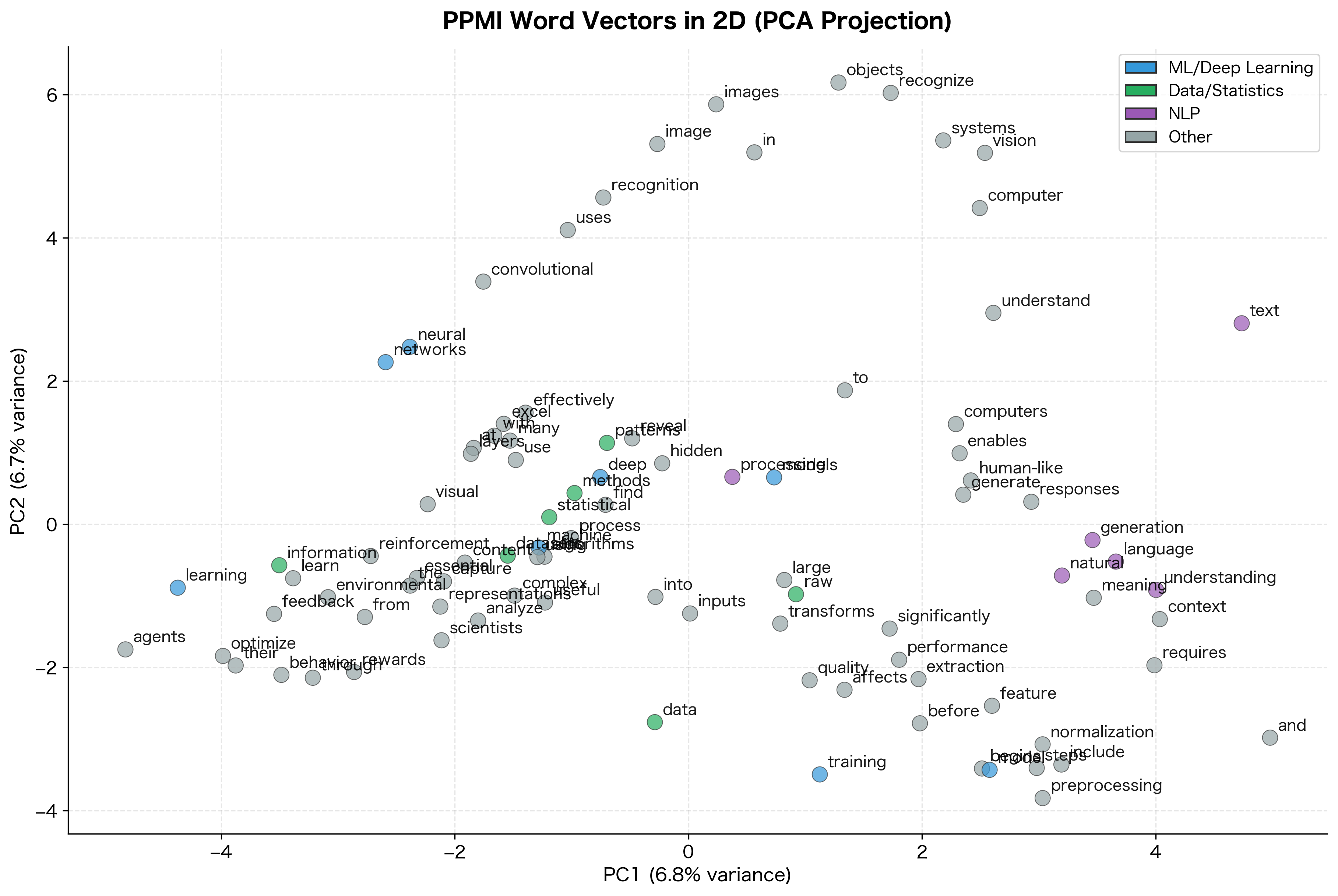
The 2D projection reveals the semantic structure captured by PPMI vectors. Even with our small corpus, related words cluster together: machine learning terms form one group, data-related terms another. This is the distributional hypothesis in action. Words with similar meanings appear in similar contexts, leading to similar PPMI vectors.
Collocation Extraction with PMI
One of PMI's most practical applications is identifying collocations: word combinations that occur together more than chance would predict. Collocations include compound nouns ("ice cream"), phrasal verbs ("give up"), and idiomatic expressions ("kick the bucket").
Collocations are word combinations whose meaning or frequency cannot be predicted from the individual words alone. PMI helps identify these by measuring which word pairs co-occur significantly more than their individual frequencies would suggest.
The top collocations are meaningful multi-word expressions like "machine learning," "neural networks," and "language models." PMI successfully identifies these as units that co-occur far more than chance would predict. The high PMI scores (often above 4) indicate these word pairs appear together 16 or more times more frequently than their individual frequencies would suggest.
The collocations table confirms that technical compound terms like "neural networks" and "machine learning" have exceptionally high PMI scores, identifying them as genuine multi-word units in this domain.
Implementation: Building a Complete PPMI Pipeline
Let's put everything together into a complete, reusable implementation for computing PPMI matrices from text.
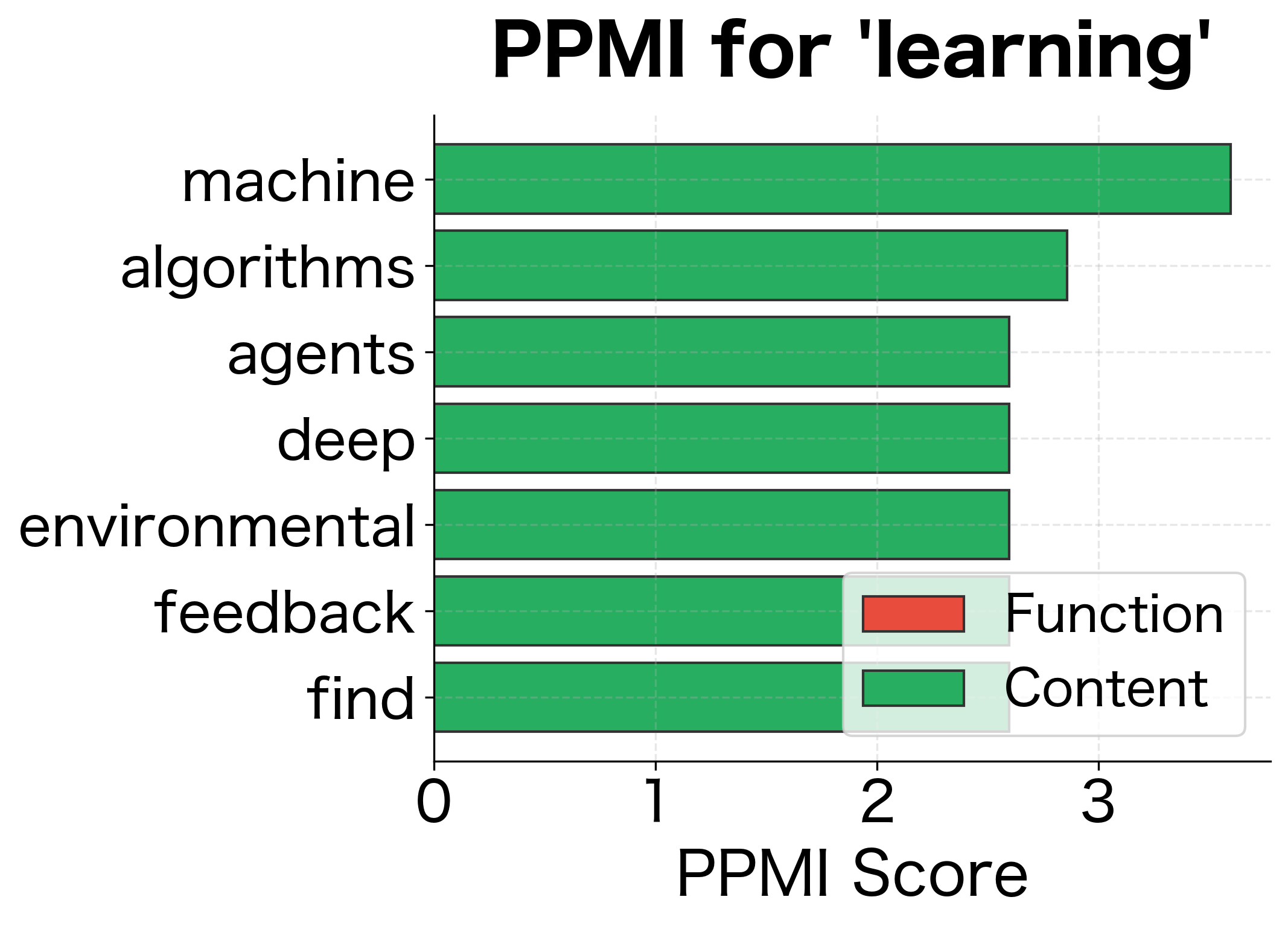
The vectorizer identifies semantically related words based on shared context patterns. For example, "learning" associates with related machine learning terms, while "data" connects to words from the data processing domain. The similarity scores (ranging from 0 to 1 for cosine similarity) reflect how closely the context distributions match between words.
Limitations and When to Use PMI
While PMI is powerful, it has limitations you should understand.
Sensitivity to Low Counts
PMI estimates are unreliable for rare word pairs. A word pair that co-occurs once when we expected 0.5 co-occurrences gets PMI of 1, but this could easily be noise. The standard solution is to require minimum co-occurrence counts before computing PMI.
The minimum count threshold removes word pairs that co-occur too rarely to provide reliable PMI estimates. The filtered entries may represent genuine but rare associations, or they may be sampling artifacts. In practice, this trade-off between precision and recall depends on corpus size and downstream application requirements.
Bias Toward Rare Words
PMI tends to give high scores to rare word pairs. If a rare word appears only in specific contexts, it gets high PMI with those contexts even if the association is coincidental. Shifted PPMI helps by raising the threshold for positive associations.
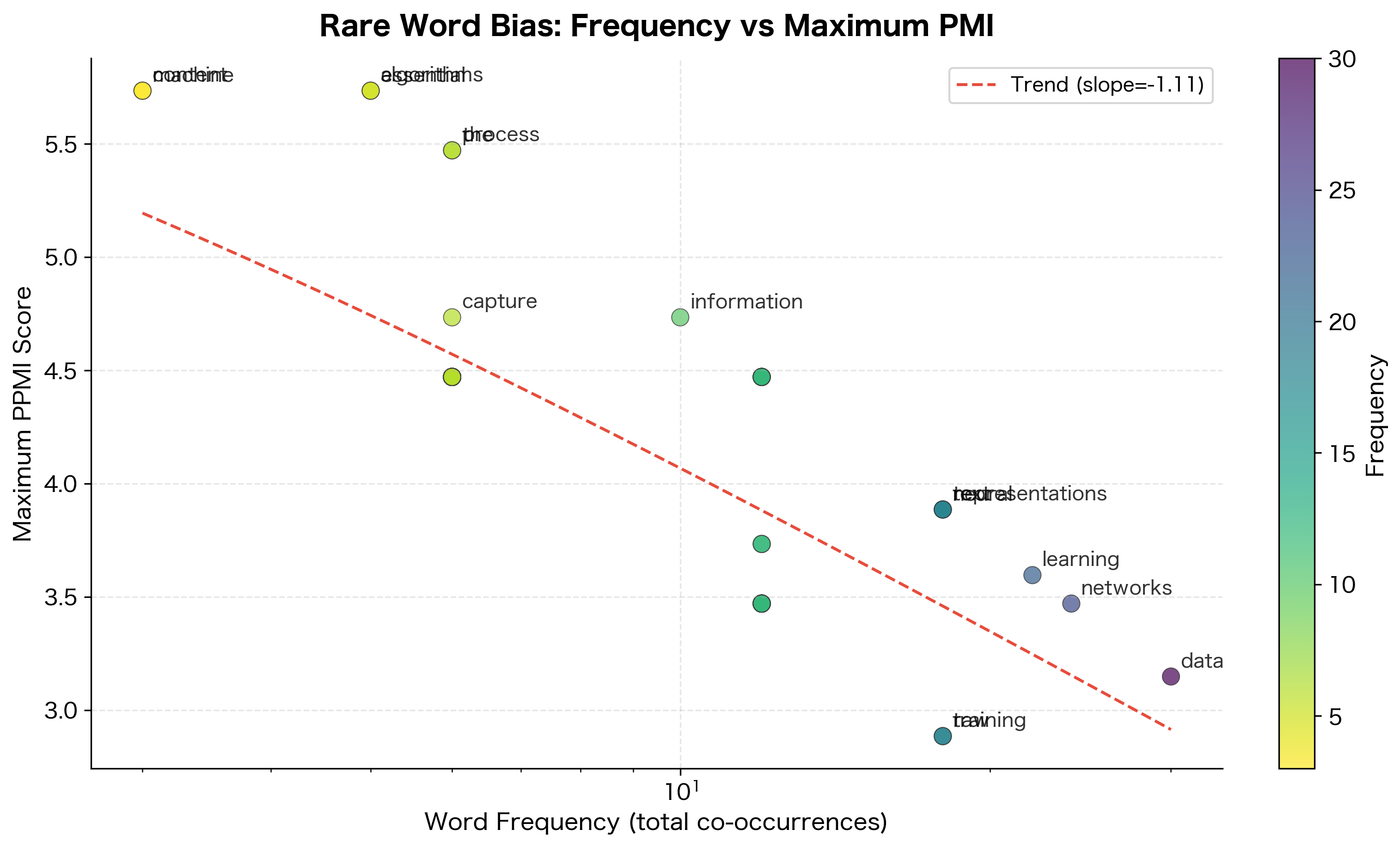
The downward trend confirms the rare word bias: words with fewer total co-occurrences tend to achieve higher maximum PMI scores. This happens because rare words have limited contexts, making each co-occurrence count proportionally more.
Computational Cost
For large vocabularies, PMI matrices become enormous. A 100,000-word vocabulary produces a 10-billion-cell matrix. While the matrix is sparse after PPMI transformation, the intermediate computations can be expensive. Practical implementations use sparse matrix formats and streaming algorithms.
When to Use PMI
PMI and PPMI are excellent choices when:
- You need interpretable association scores between words
- You're extracting collocations or multi-word expressions
- You want sparse, high-dimensional word vectors as input to other algorithms
- You need a baseline to compare against neural embeddings
- Computational resources are limited (no GPU required)
Neural methods like Word2Vec often outperform PPMI for downstream tasks, but the difference is smaller than you might expect. For many applications, PPMI provides a strong, interpretable baseline.
Summary
Pointwise Mutual Information transforms raw co-occurrence counts into meaningful association scores by comparing observed co-occurrence to what we'd expect under independence.
Key concepts:
- PMI formula:
measures how much more (or less) two words co-occur than chance would predict, where is the joint probability of co-occurrence and is the expected probability under independence.
-
Positive PMI (PPMI): clips negative values to zero, keeping only positive associations. This produces sparse matrices that work well with machine learning algorithms.
-
Shifted PPMI: subtracts before clipping, filtering out weak associations. Connected theoretically to Word2Vec's negative sampling.
-
PMI interpretation: Positive PMI means words co-occur more than expected (strong association). Zero means independence. Negative means avoidance.
Practical applications:
- Collocation extraction: Finding meaningful multi-word expressions
- Word similarity: Using PPMI vectors with cosine similarity
- Feature weighting: PPMI as a preprocessing step before dimensionality reduction
Key Parameters
| Parameter | Typical Values | Effect |
|---|---|---|
window_size | 2-5 | Larger windows capture broader topical context but may include more noise; smaller windows emphasize syntactic relationships |
min_count | 2-10 | Higher values filter unreliable associations from rare words; start with 2-5 for small corpora, 5-10 for larger ones |
shift_k | 1-15 | Higher values keep only the strongest associations; k=5 is common and corresponds to Word2Vec's default negative sampling |
Guidelines for choosing each parameter:
-
window_size: Smaller windows (2-3) tend to capture syntactic relationships and function word patterns. Larger windows (5-10) capture more topical or semantic relationships. For most NLP applications, a window of 2-5 provides a good balance. -
min_count: This threshold depends on corpus size. For small corpora (under 1 million words), use 2-5. For larger corpora, 5-10 reduces noise from rare co-occurrences. Higher thresholds produce more reliable but potentially incomplete association matrices. -
shift_k: The shift parameter controls sensitivity. With k=1 (standard PPMI), all positive associations are retained. With k=5, only associations at least 5 times stronger than expected survive. If downstream tasks show signs of noise from rare word artifacts, increase k.
The next chapter shows how to reduce the dimensionality of PPMI matrices using Singular Value Decomposition, producing dense vectors that capture the essential structure in fewer dimensions.
Quiz
Ready to test your understanding? Take this quick quiz to reinforce what you've learned about Pointwise Mutual Information and word associations.

Comments