Word Embedding Evaluation: Intrinsic & Extrinsic Methods with Bias Detection

Embedding EvaluationLink Copied

You've trained a word embedding model. The loss converged, the code ran without errors, and you have a matrix of 300-dimensional vectors. But how do you know if these embeddings are any good? What makes one set of embeddings better than another?

Evaluating word embeddings is surprisingly nuanced. Unlike classification tasks where accuracy provides a clear metric, embedding quality is multidimensional. Embeddings might excel at capturing analogies but fail at word similarity. They might perform brilliantly on sentiment analysis but contain harmful biases. The right evaluation depends entirely on how you plan to use the embeddings.

This chapter develops a comprehensive evaluation toolkit. We'll explore intrinsic evaluations that probe the embedding space directly, extrinsic evaluations that measure downstream task performance, visualization techniques for qualitative inspection, and methods for detecting embedded biases. By the end, you'll have the tools to rigorously assess any word embedding model.

Intrinsic vs Extrinsic EvaluationLink Copied

The fundamental split in embedding evaluation is between intrinsic and extrinsic methods. Understanding this distinction is crucial for interpreting evaluation results.

The relationship between intrinsic and extrinsic performance is complex and sometimes counterintuitive. Research has shown that embeddings with higher intrinsic scores don't always perform better on downstream tasks. This disconnect arises because intrinsic tests capture specific linguistic properties, while downstream tasks may require different capabilities.

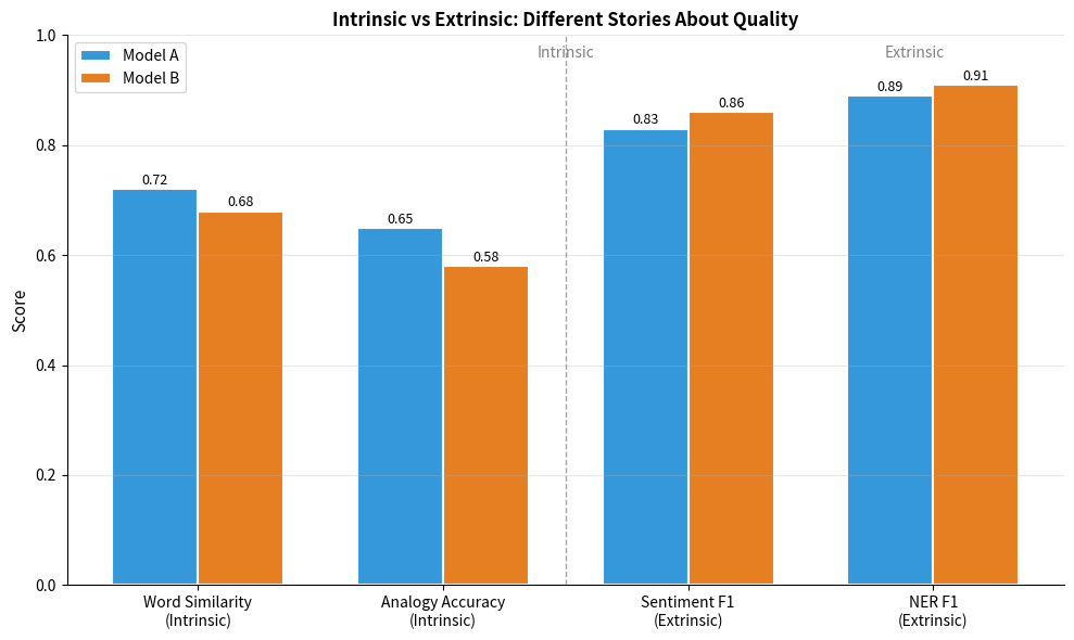
This example illustrates a common scenario: Model A achieves higher intrinsic scores, but Model B performs better on downstream tasks. If you're building a sentiment classifier, Model B is clearly the better choice, despite its lower analogy accuracy.

The practical takeaway: always include extrinsic evaluations relevant to your use case. Intrinsic metrics provide useful diagnostic information, but they don't tell the whole story.

Word Similarity EvaluationLink Copied

The most established intrinsic evaluation is word similarity. Humans rate the semantic similarity of word pairs on a scale (typically 0-10), and we measure how well embedding cosine similarities correlate with these human judgments.

Standard DatasetsLink Copied

Several benchmark datasets have become standard for word similarity evaluation:

WordSim-353 contains 353 word pairs rated by 13-16 human annotators. It mixes similarity (synonymy) and relatedness (associated but not similar). "Cup" and "coffee" are related but not similar. "Car" and "automobile" are both related and similar.

SimLex-999 addresses WordSim's conflation of similarity and relatedness. Its 999 pairs focus specifically on genuine similarity: words that could be substituted for each other. It's harder than WordSim because relatedness doesn't count.

MEN contains 3,000 pairs covering a range of parts of speech. Ratings come from crowd workers rather than expert annotators.

Computing Similarity CorrelationsLink Copied

The evaluation process involves two key measurements that work together to tell us how well embeddings capture human intuitions about word similarity.

First, we compute the cosine similarity between each word pair's embeddings. Cosine similarity measures the angle between two vectors, ignoring their magnitudes. Two vectors pointing in similar directions have high cosine similarity (close to 1), while perpendicular vectors have similarity near 0. For word embeddings, high cosine similarity indicates that two words appear in similar contexts and likely share related meanings.

Second, we calculate the Spearman correlation between these embedding similarities and the human ratings. Why Spearman rather than Pearson? Spearman correlation measures whether the rankings match, not whether the actual values align linearly. This is exactly what we want: if humans rank "happy/cheerful" as more similar than "dog/cat", we care whether embeddings agree with that ordering, regardless of the exact numerical values. Spearman correlation ranges from -1 (perfect inverse ranking) through 0 (no relationship) to +1 (perfect agreement).

The Spearman correlation measures how well the embedding-based rankings match human rankings. A correlation above 0.7 indicates that the embeddings preserve human similarity intuitions reasonably well. The p-value tells us whether this correlation is statistically significant (values below 0.05 indicate significance).

Let's examine the individual similarities to understand what the embeddings capture:

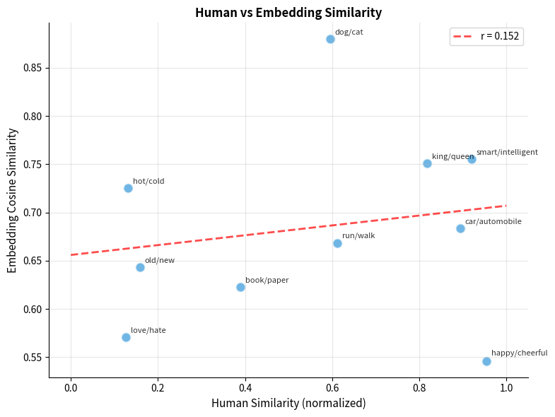
The scatter plot reveals both strengths and limitations. High-similarity pairs like "happy/cheerful" and "smart/intelligent" score high on both scales. Antonyms like "hot/cold" receive low human ratings but may have moderate embedding similarity because they appear in similar contexts (both are temperature words).

SimLex vs WordSim: Similarity vs RelatednessLink Copied

The distinction between similarity and relatedness is crucial. "Coffee" and "cup" are highly related but not similar. You can't substitute one for the other. SimLex-999 was specifically designed to test genuine similarity.

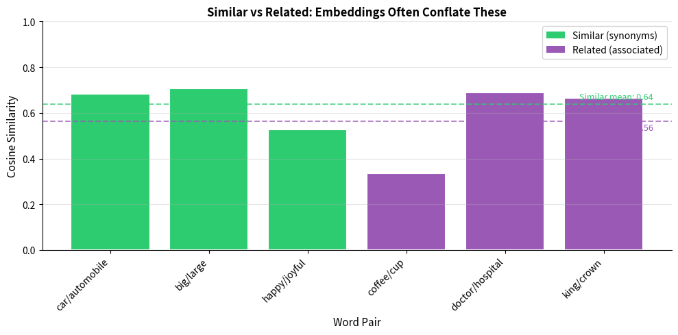
Standard word embeddings trained on co-occurrence tend to conflate similarity and relatedness because related words appear in similar contexts. This is why SimLex-999 is a harder benchmark. If you need embeddings that distinguish these concepts, you may need specialized training objectives.

Word Analogy EvaluationLink Copied

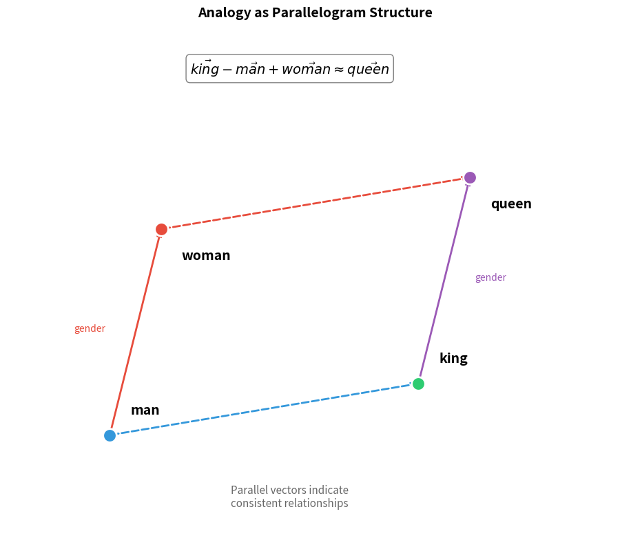
The analogy task tests whether embeddings capture semantic relationships through vector arithmetic. The classic example: "king - man + woman ≈ queen." If the embedding space encodes gender as a consistent direction, this arithmetic should work.

The Analogy TaskLink Copied

At first glance, the idea that you can do arithmetic with words seems almost magical. How can you subtract "man" from "king" and add "woman" to get "queen"? The key insight is that word embeddings aren't just arbitrary numbers assigned to words. They're geometric representations where directions carry meaning.

Think of it this way: if the embedding space has learned that "male" and "female" represent opposite ends of a direction (let's call it the gender axis), then moving from "man" to "woman" means traveling along that axis. Similarly, moving from "king" to "queen" should involve the same directional shift. If both relationships encode the same underlying concept (gender), their vector differences should be parallel.

This observation leads to a simple but powerful formula. Given three words A, B, and C, we want to find word D such that "A is to B as C is to D." The relationship between A and B is captured by the vector difference $\mathbf{b} - \mathbf{a}$. If the same relationship holds between C and D, then D should be located at:

where:

• $\mathbf{a}$, $\mathbf{b}$, $\mathbf{c}$: embedding vectors for words A, B, and C
• $\mathbf{b} - \mathbf{a}$: the relationship vector (what transforms A into B)
• $\mathbf{d}$: target vector representing the expected embedding for word D

The formula reads as: "Start at C, then apply the same transformation that takes A to B." We find D by locating the word whose embedding is closest to this computed vector (excluding A, B, and C to prevent trivial solutions).

This geometric property only works if the embedding space has organized itself so that analogous relationships point in consistent directions. When it works, it's evidence that the embeddings have captured genuine semantic structure. When it fails, it often reveals that the relationship isn't as consistent as we assumed, or that the training data didn't provide enough examples for the model to learn it.

Analogy CategoriesLink Copied

The Google Analogy Test Set contains approximately 19,500 analogies across two categories:

Semantic analogies test factual relationships:

• Capital-country: Paris : France :: Tokyo : Japan
• Currency: dollar : USA :: euro : Europe
• Gender: king : queen :: man : woman

Syntactic analogies test grammatical relationships:

• Tense: walk : walked :: run : ran
• Plural: cat : cats :: dog : dogs
• Comparative: big : bigger :: small : smaller

The accuracy breakdown reveals which relationship types the embeddings capture best. Syntactic analogies often achieve higher accuracy because grammatical patterns appear consistently in text. Semantic analogies like capital-country relationships may vary more depending on how well-represented each entity is in the training corpus.

Limitations of Analogy EvaluationLink Copied

While analogy tasks are popular, they have significant limitations:

1. Sensitivity to dataset: Performance varies dramatically across different analogy sets
2. Only tests specific relationships: Good analogy performance doesn't guarantee general embedding quality
3. Artifacts of training data: Some analogies work because of corpus biases, not linguistic understanding
4. Unclear relevance: Analogy performance often doesn't correlate with downstream task performance

Embedding VisualizationLink Copied

Visualization provides qualitative insights that quantitative metrics miss. By projecting high-dimensional embeddings to 2D or 3D, we can observe clustering patterns, outliers, and relationships.

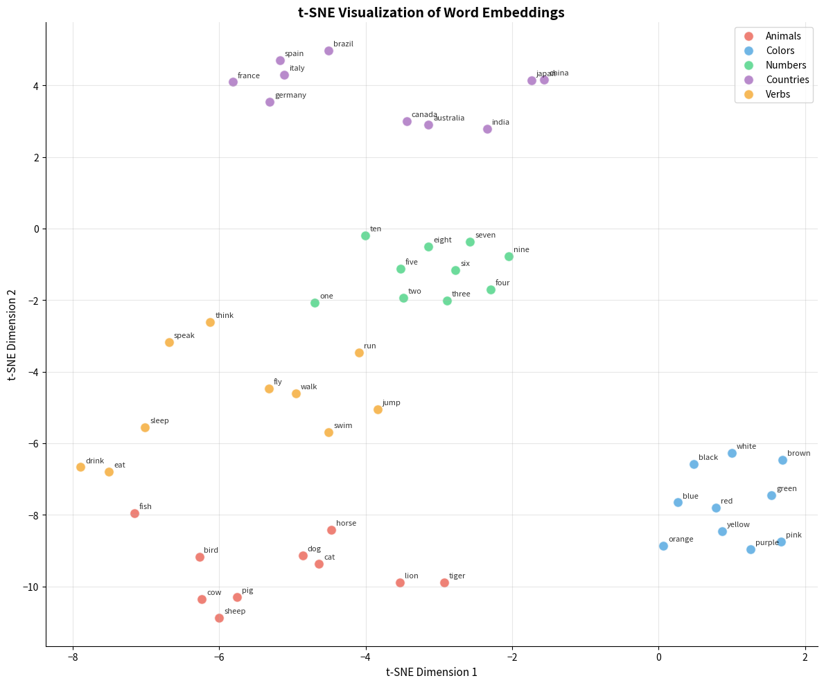
t-SNE VisualizationLink Copied

t-Distributed Stochastic Neighbor Embedding (t-SNE) is the most popular technique for embedding visualization. It preserves local structure: words that are close in high-dimensional space remain close in the projection.

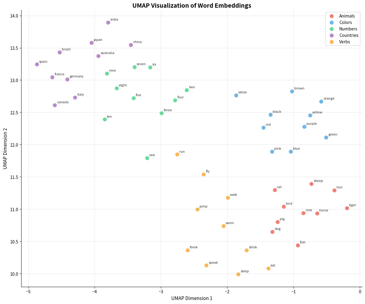
UMAP as an AlternativeLink Copied

Uniform Manifold Approximation and Projection (UMAP) is a newer alternative to t-SNE. It's faster, better preserves global structure, and produces more reproducible results.

Visualization CaveatsLink Copied

While visualization is valuable for building intuition, it has important limitations:

1. Projection distortion: Reducing from 100+ dimensions to 2 inevitably loses information
2. Non-determinism: t-SNE and UMAP can produce different layouts on different runs
3. Perplexity/neighbor sensitivity: Results depend heavily on hyperparameter choices
4. Misleading distances: Distances between clusters in the visualization may not reflect true embedding distances

Use visualization for exploration and communication, but don't make quantitative claims based on 2D projections.

Downstream Task EvaluationLink Copied

The ultimate test of embeddings is performance on real tasks. Let's evaluate embeddings on text classification, a common downstream application.

Topic ClassificationLink Copied

We'll use the 20 Newsgroups dataset to evaluate how well embeddings support text classification. This dataset contains posts from different newsgroups, making it ideal for testing whether embeddings capture topical information.

The high accuracy demonstrates that even simple mean-pooled embeddings can capture enough semantic information for topic classification. The key advantage of this evaluation approach is that it directly measures what matters: whether the embeddings help solve real tasks. If your application involves document classification, these results are far more relevant than intrinsic metrics.

Comparison Across TasksLink Copied

A thorough extrinsic evaluation tests embeddings across multiple tasks:

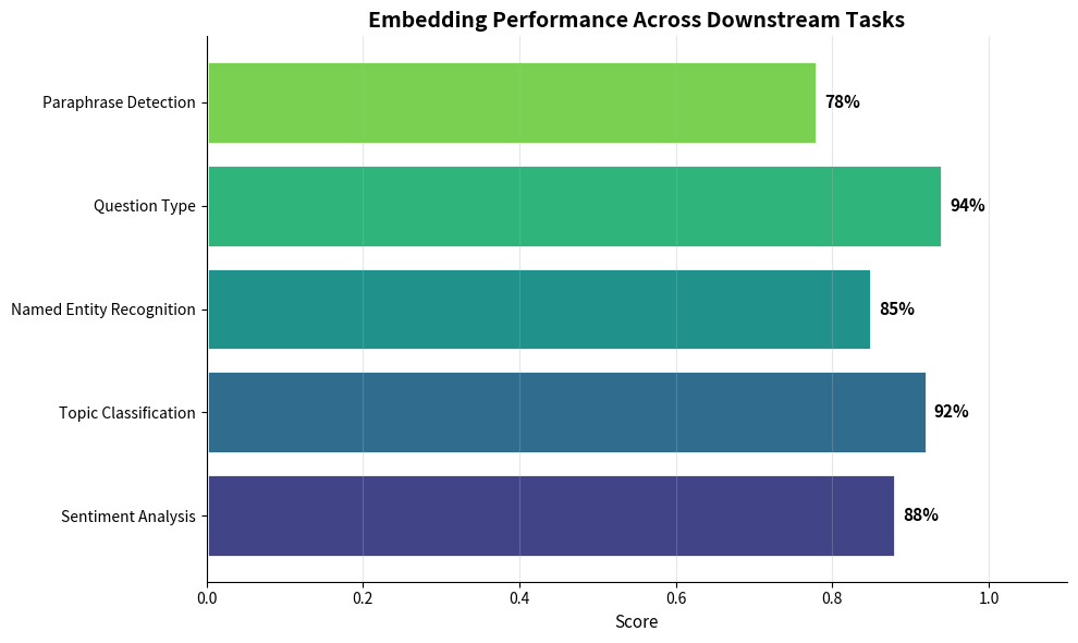
The variation across tasks highlights why no single metric captures embedding quality. Choose evaluation tasks that match your intended application.

Embedding Bias DetectionLink Copied

Word embeddings learn from human-generated text, and human text contains biases. These biases become encoded in the embedding geometry, potentially amplifying harmful stereotypes in downstream applications.

Detecting Gender BiasLink Copied

The most studied bias in word embeddings is gender bias. The key insight is that we can use the same geometric properties that make embeddings useful for analogies to detect problematic associations.

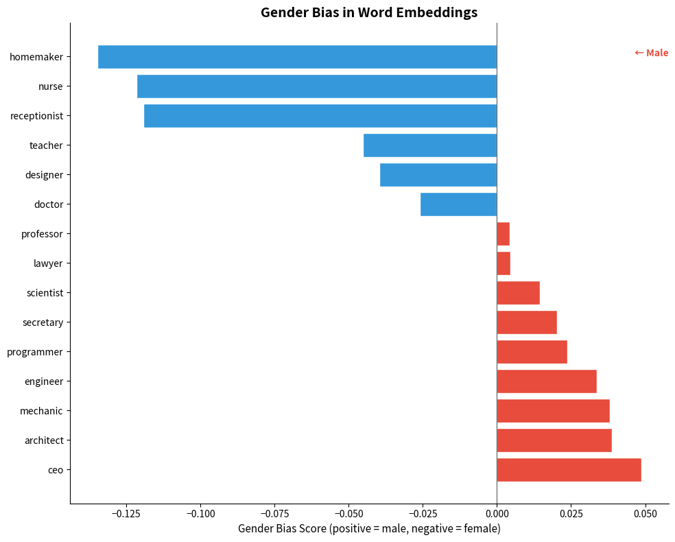
Consider an occupation word like "engineer." In an ideal world, this word should be equidistant from "he" and "she" since engineering has no inherent gender. But if the training corpus contains more sentences like "He is an engineer" than "She is an engineer," the embedding for "engineer" will drift closer to male-associated terms.

We can measure this drift with a simple bias score: compute the cosine similarity between a word and male terms, subtract the similarity to female terms. A score of zero means perfect balance. Positive scores indicate male association; negative scores indicate female association. By averaging across multiple gendered word pairs (he/she, man/woman, male/female), we reduce noise from any single comparison.

The bias scores reveal systematic associations between occupations and gender. Occupations like "engineer" and "programmer" show positive scores (male association), while "nurse" and "secretary" show negative scores (female association). These patterns reflect stereotypes present in the training text, not any inherent truth about these professions.

Word Embedding Association Test (WEAT)Link Copied

While individual bias scores reveal patterns, we need a more rigorous framework to quantify bias in a statistically meaningful way. The Word Embedding Association Test (WEAT) provides exactly this, drawing inspiration from psychology's Implicit Association Test (IAT).

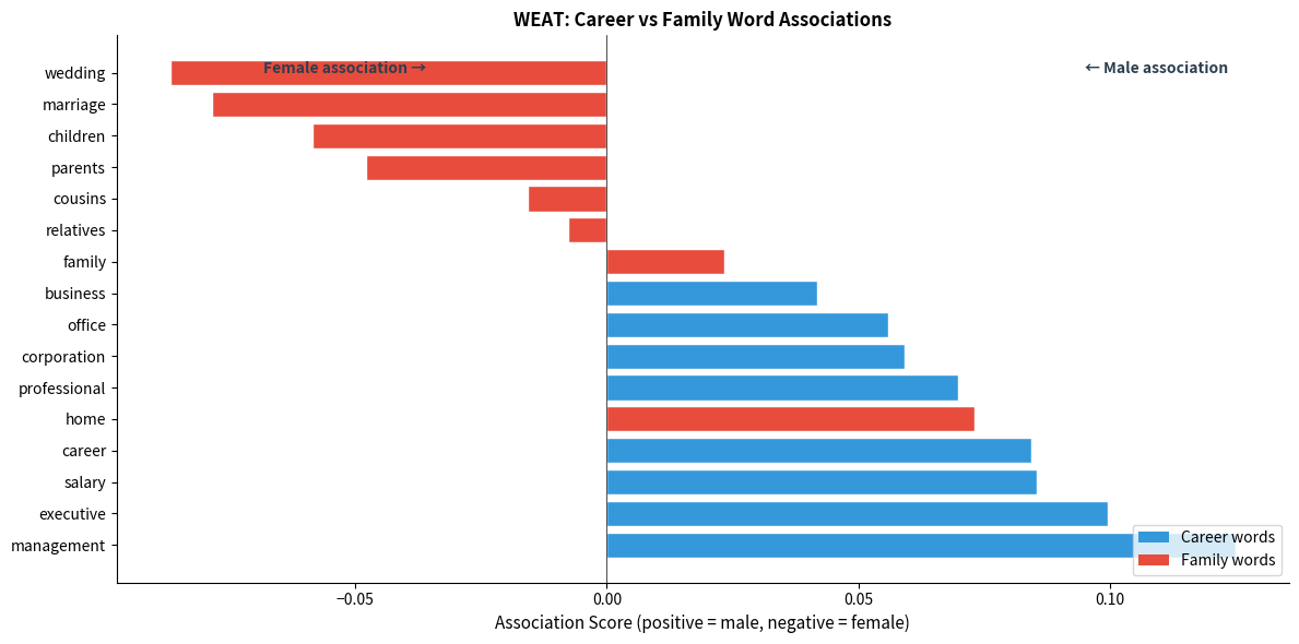
The core idea is elegant: if embeddings are unbiased, two conceptually neutral word sets (like careers and family) should associate equally with two attribute sets (like male and female terms). Any systematic difference indicates bias.

Here's how WEAT works step by step:

1. Define target word sets: Two sets we want to test for differential association. For example, career words (executive, salary, office) versus family words (home, parents, children).

2. Define attribute word sets: Two sets representing the dimension we're measuring bias along. For gender bias: male attributes (he, man, boy) versus female attributes (she, woman, girl).

3. Compute association scores: For each target word, calculate how much more it associates with one attribute set than the other. A career word that's closer to male terms than female terms receives a positive association score.

4. Compare target sets: The key question is whether one target set (careers) systematically associates more with one attribute set (male) than the other target set (family) does.

5. Compute effect size: The final WEAT score uses Cohen's d, a standardized measure of the difference between the two target sets' mean associations, divided by the pooled standard deviation. This normalization makes the score interpretable across different embedding models and word sets.

Implications of Embedded BiasLink Copied

Bias in embeddings has real-world consequences:

1. Resume screening: Systems using biased embeddings may rank male candidates higher for technical roles
2. Search engines: Queries for "CEO" might surface more male images
3. Machine translation: Gender-neutral terms might be translated with stereotypical gender
4. Sentiment analysis: Texts about certain demographic groups might receive biased sentiment scores

Bias detection should be part of any responsible embedding evaluation pipeline. Debiasing techniques exist but have limitations, so awareness and mitigation strategies are essential.

Evaluation PitfallsLink Copied

Even with the right metrics, embedding evaluation can go wrong. Here are common pitfalls to avoid:

1. Vocabulary Coverage IssuesLink Copied

Many evaluation datasets contain rare or archaic words missing from embedding vocabularies. Simply skipping these words can inflate scores.

Rare or specialized words often missing from embedding vocabularies can skew evaluation results. If your evaluation set contains many such words and you simply exclude them, you're only testing on common words where embeddings typically perform better. Always report coverage alongside performance metrics.

2. Dataset ContaminationLink Copied

If your embeddings were trained on text that includes the evaluation data, results are misleadingly optimistic.

3. Hyperparameter SensitivityLink Copied

Results can vary significantly with hyperparameters like the number of neighbors for nearest neighbor searches, or thresholds for similarity judgments.

4. Cherry-Picking CategoriesLink Copied

Reporting only the best-performing analogy or similarity categories creates a misleading picture. Always report aggregate scores.

5. Ignoring Statistical SignificanceLink Copied

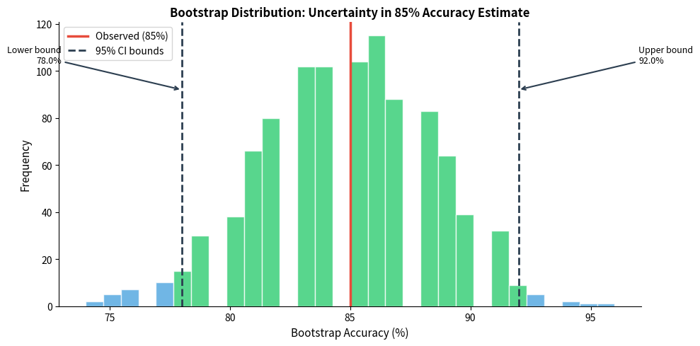
Small test sets can produce unreliable results. An accuracy of 85% on 100 test cases doesn't mean your model is exactly 85% accurate on all possible inputs. It's an estimate with uncertainty, and that uncertainty shrinks as you test on more examples.

Bootstrap confidence intervals offer a practical way to quantify this uncertainty. The idea is simple: resample your test results with replacement many times, compute the mean each time, and observe the distribution. The range containing 95% of these bootstrap means gives you a 95% confidence interval. If two models' confidence intervals don't overlap, you have evidence of a real difference.

Building an Evaluation PipelineLink Copied

Let's bring everything together into a reusable evaluation framework.

The evaluation pipeline produces a consolidated view of embedding performance across all dimensions. This modular approach allows you to add new evaluation methods as needed while maintaining a consistent reporting format.

Key ParametersLink Copied

When evaluating word embeddings, several parameters and choices significantly impact your results:

Word Similarity Evaluation

• Correlation metric: Spearman correlation (rank-based) is preferred over Pearson because it doesn't assume linearity between human scores and cosine similarities
• Dataset choice: SimLex-999 for pure similarity, WordSim-353 for similarity + relatedness, MEN for broader coverage

Analogy Evaluation

• Vocabulary search space: Limiting search to top-N frequent words (e.g., 50,000) balances accuracy with computation time
• Exclusion set: Always exclude the input words (a, b, c) from candidate answers to avoid trivial solutions

Visualization (t-SNE)

• perplexity: Controls the balance between local and global structure. Typical values: 5-50. Lower values emphasize local clusters, higher values show more global structure
• n_iter: Number of optimization iterations. Default 1000 is usually sufficient, but complex datasets may need more
• random_state: Set for reproducibility, as t-SNE is non-deterministic

Visualization (UMAP)

• n_neighbors: Number of neighbors for local structure. Higher values (15-50) preserve more global structure
• min_dist: Controls how tightly points cluster. Lower values (0.0-0.1) create denser clusters

Bias Detection

• Attribute word sets: Use multiple word pairs per concept (e.g., he/she, man/woman, male/female) to reduce noise from individual word idiosyncrasies
• Effect size thresholds: Cohen's d benchmarks: < 0.2 negligible, 0.2-0.5 small, 0.5-0.8 medium, > 0.8 large

Downstream Evaluation

• Aggregation method: Mean pooling is standard, but max pooling sometimes works better for sentiment tasks
• Classifier choice: Logistic regression provides a clean baseline; more complex models may overfit to artifacts rather than embedding quality

SummaryLink Copied

Evaluating word embeddings requires a multi-faceted approach. No single metric captures embedding quality completely.

Key takeaways:

1. Intrinsic vs extrinsic: Intrinsic evaluations (similarity, analogies) are fast and interpretable but may not predict downstream performance. Always include task-specific extrinsic evaluations.

2. Word similarity: Spearman correlation with human similarity judgments remains the standard intrinsic test. SimLex-999 tests genuine similarity, while WordSim-353 conflates similarity with relatedness.

3. Analogies: Vector arithmetic captures some semantic relationships, but analogy accuracy has limited correlation with real-world usefulness.

4. Visualization: t-SNE and UMAP reveal clustering structure but introduce projection distortions. Use for exploration, not quantitative claims.

5. Downstream tasks: The ultimate test is performance on your intended application. Classification, NER, and other tasks provide direct measures of utility.

6. Bias detection: Embeddings encode societal biases. WEAT and association tests can quantify these biases, which is essential for responsible deployment.

7. Pitfalls: Watch for vocabulary coverage issues, dataset contamination, hyperparameter sensitivity, and statistical significance. Report aggregate results, not cherry-picked categories.

The goal isn't perfect scores on every metric but rather understanding what your embeddings capture and whether it matches your needs. A model with lower intrinsic scores might be the right choice if it excels at your specific task. Evaluation is ultimately about making informed decisions.

QuizLink Copied

Ready to test your understanding? Take this quick quiz to reinforce what you've learned about evaluating word embeddings.