FastText: Subword Embeddings for OOV Words & Morphology

FastTextLink Copied

Word2Vec revolutionized word embeddings by learning dense vector representations from context. But it has a fundamental limitation: each word is treated as an atomic unit. The embedding for "running" shares nothing with "run," "runner," or "runs." Every word form needs to be seen during training to get a representation, and words absent from the training corpus receive no embedding at all.

This poses serious challenges for morphologically rich languages like German, Finnish, or Turkish, where a single root can spawn thousands of word forms through compounding and inflection. Even in English, rare words, typos, and domain-specific terms often lack embeddings despite being clearly related to known words.

FastText, introduced by Bojanowski et al. at Facebook AI Research in 2017, solves this elegantly: instead of treating words as atomic, it represents each word as a bag of character n-grams. The word "running" becomes a collection of substrings like "run," "unn," "nni," "nin," "ing," plus boundary markers. The word's embedding is simply the sum of its n-gram embeddings. This simple change unlocks three powerful capabilities: handling out-of-vocabulary words, capturing morphological patterns, and improving representations for rare words.

This chapter develops FastText from the ground up. We'll understand why subword representations matter, work through the architecture and training process, and implement a working FastText model that handles words it has never seen.

The Vocabulary Problem in Word2VecLink Copied

Before diving into FastText's solution, let's understand the problem it addresses. Word2Vec models learn one embedding per vocabulary entry. If a word wasn't in the training data, it has no representation.

The vocabulary problem becomes severe in three scenarios:

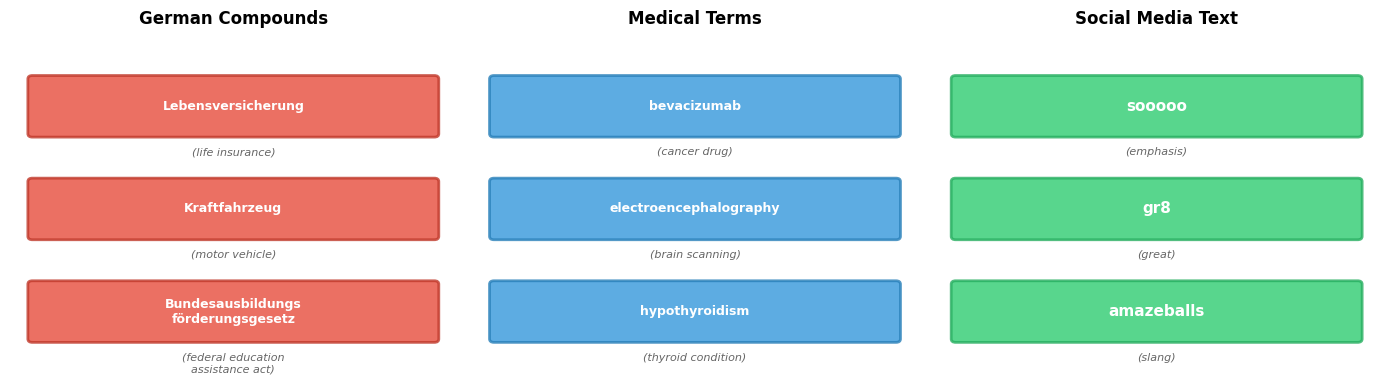
Morphologically rich languages: German compounds like "Lebensversicherungsgesellschaft" (life insurance company) or Finnish cases like "talossanikinko" (in my house, too?) generate enormous vocabularies. Training a model that sees every possible form is impractical.

Domain-specific text: Medical terms, product names, or technical jargon often don't appear in general-purpose training corpora. A model trained on news articles won't have embeddings for "bevacizumab" or "iPhone15ProMax."

Noisy text: Social media, user reviews, and informal writing contain typos, creative spellings, and neologisms. "Cooool," "gr8," and "amaziiing" are meaningful but likely absent from formal training data.

The FastText Solution: Character N-gramsLink Copied

Word2Vec treats each word as an indivisible symbol. "Running" and "runner" share nothing in their representations despite their obvious linguistic relationship. This atomic view ignores the internal structure of words, structure that humans naturally exploit when encountering unfamiliar terms. When you see "unfamiliar," you don't need to have seen it before to guess its meaning: the prefix "un-" signals negation, and you recognize the root "familiar."

FastText captures this intuition algorithmically. Instead of treating words as atomic symbols, it represents each word as a bag of character n-grams, overlapping substrings of characters. The word's embedding emerges from combining the embeddings of its constituent parts.

Why this representation? Consider what happens when two words share the same root. "Running" and "runner" both contain the substrings "run," "unn," and several others. If these shared substrings contribute to both words' embeddings, then related words will naturally have similar representations. This happens not because we explicitly encode morphological rules, but because the overlapping structure emerges from the character sequences themselves.

The decomposition process transforms each word through three steps:

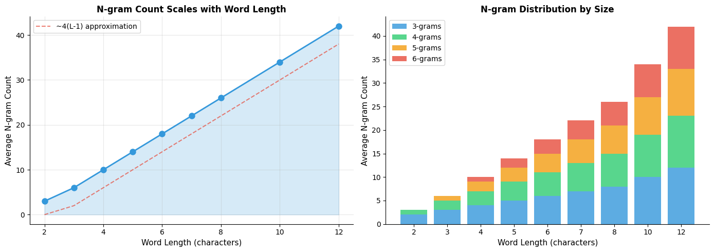
1. Add boundary markers: "where" → "" (these mark word boundaries, distinguishing prefixes from suffixes)
2. Extract all n-grams: Generate all substrings of length $n$ within the configured range (typically 3 to 6)
3. Include the word itself: The full word acts as an additional feature for known vocabulary items

The word "where" decomposes into 18 n-grams spanning lengths 3 to 6. This decomposition reveals something important: different n-grams encode different aspects of the word. The boundary markers "<wh" and "re>" capture positional information: "<wh" signals a word beginning, while "re>" indicates a word ending. Meanwhile, the n-gram "her" floating in the middle carries no positional constraints.

Why Boundary Markers MatterLink Copied

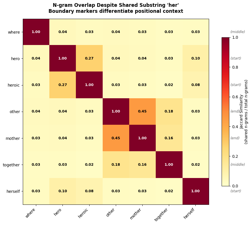
This positional encoding matters more than it might first appear. Consider the substring "her" appearing in three different words: "where," "hero," and "other." Without boundary markers, these would all contribute the same n-gram "her" to each word's representation. But linguistically, these are quite different situations:

• In "hero," "her" forms the start of the word (a prefix)
• In "other," "her" ends the word (a suffix)
• In "where," "her" sits in the middle

Boundary markers disambiguate these cases:

The boundary markers ensure that "hero" (containing "<he," "her," "ero," "ro>") and "other" (containing "the," "her," "er>") produce overlapping but distinct n-gram sets. They share "her" because both contain that substring internally, but their boundary-marked n-grams differ entirely. This encoding captures both the shared internal structure and the distinct positional contexts.

From N-grams to Word EmbeddingsLink Copied

With our words decomposed into n-gram sets, we need a mechanism to combine these pieces into a single word representation. FastText takes the simplest possible approach: summation.

Each n-gram $g$ has its own learnable embedding vector $\mathbf{z}_g$. To compute a word's embedding, we simply add up all its n-gram embeddings, optionally including a word-level embedding for vocabulary words:

The components of this formula reveal FastText's elegance:

• $\mathbf{v}_w$ is the final embedding we want, the vector that will represent word $w$ in downstream tasks
• $\mathbf{z}_w$ is an optional word-level embedding that captures any meaning not encoded by subwords (for vocabulary words only)
• $G_w$ is the set of character n-grams extracted from word $w$ (the decomposition we computed above)
• $\mathbf{z}_g$ is the learned embedding for n-gram $g$, shared across all words containing that n-gram

The sum means that words sharing n-grams automatically share portions of their representation. The n-gram embeddings $\mathbf{z}_g$ are the true learned parameters. They encode character-sequence semantics that transfer across all words containing those sequences.

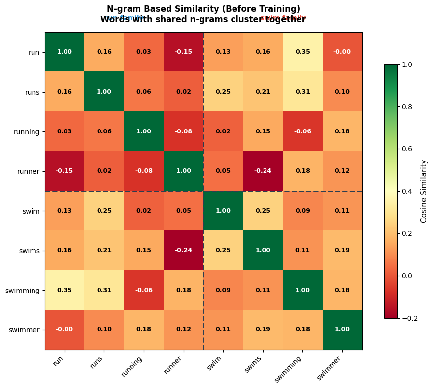
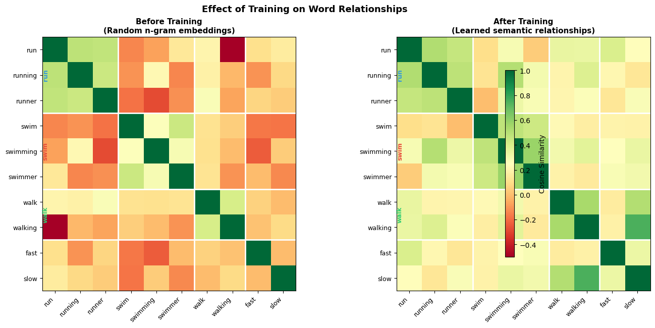
Even with random initialization, before any training has occurred, words sharing n-grams exhibit non-trivial similarity. This is the key insight: the structure of language is partially encoded in the character sequences themselves. Training amplifies this signal, making morphological variants cluster together not because we programmed morphological rules, but because the shared substrings naturally encode shared meaning.

Visualizing N-gram OverlapLink Copied

To build intuition for why this works, let's visualize which n-grams different word forms share. Consider the word family "run," "runs," "running," and "runner," all derived from the same root:

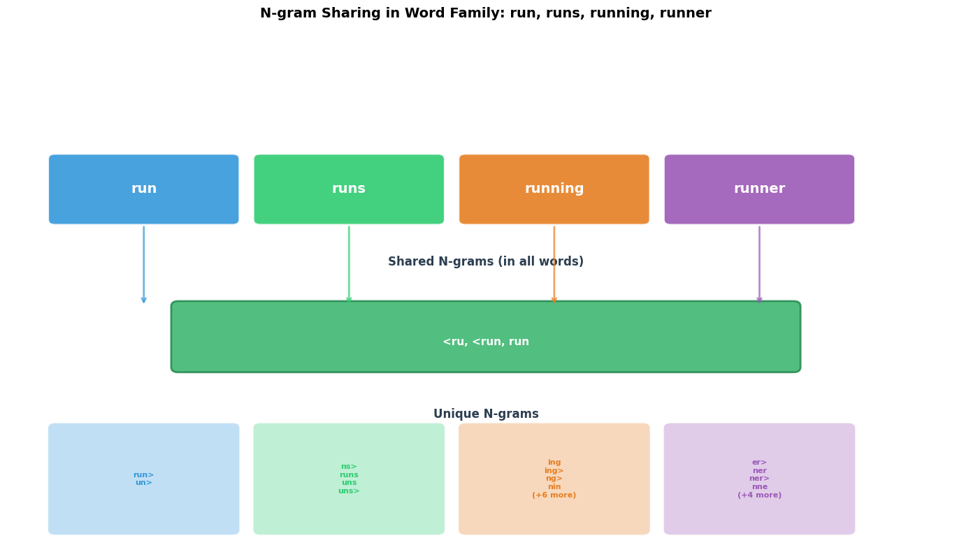
The FastText Training ObjectiveLink Copied

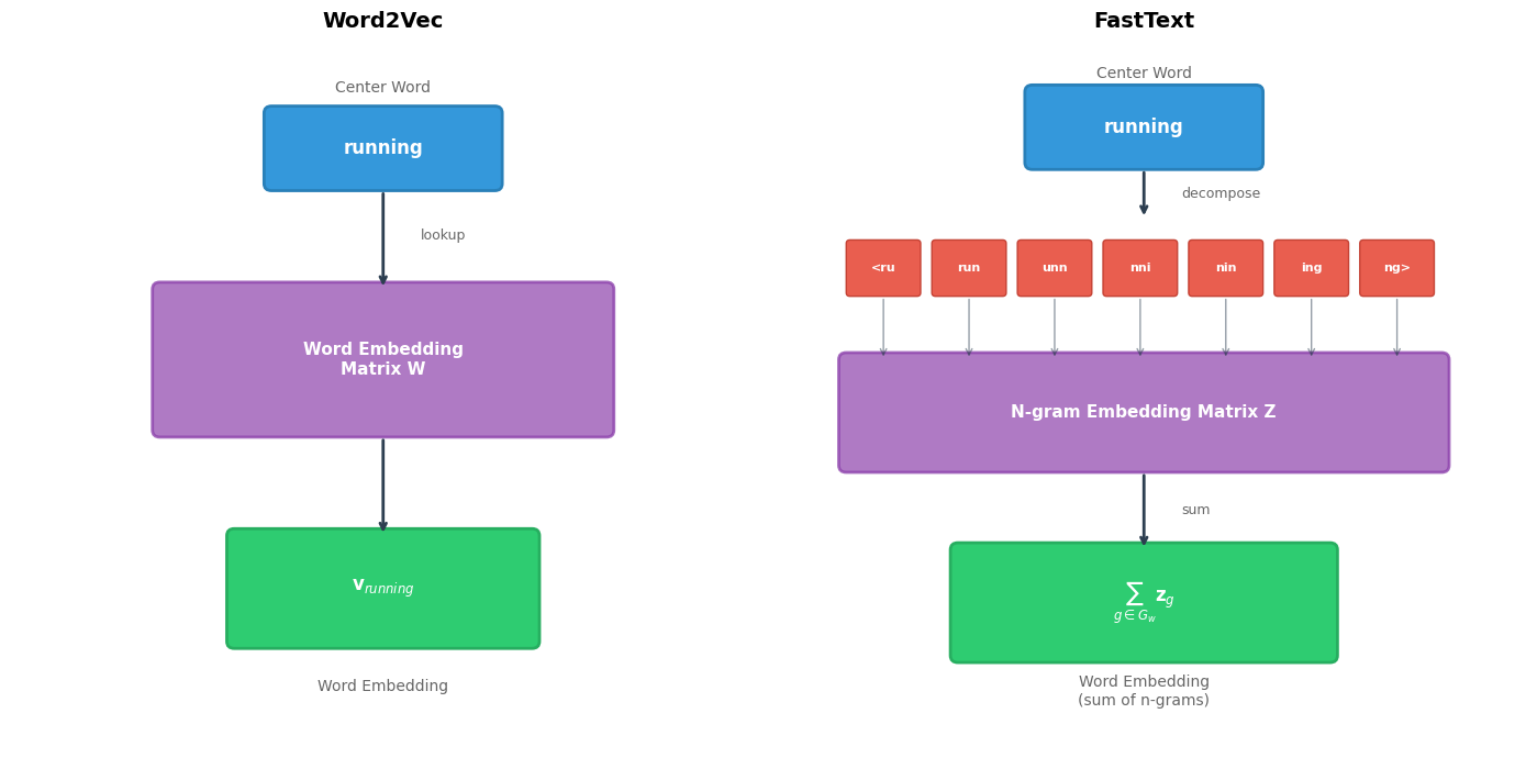
We've established how FastText represents words as sums of n-gram embeddings. But how do we learn what values those n-gram embeddings should take? The answer lies in adapting Word2Vec's Skip-gram training objective to operate on n-grams rather than words.

Recall that Skip-gram learns embeddings by predicting context words from center words. FastText uses the same principle, but with a crucial modification: instead of looking up a single embedding for the center word, we compute the center word's representation as the sum of its n-gram embeddings. This propagates gradients back to all n-grams during training, allowing them to learn from every word they appear in.

The scoring function measures how compatible a center word $w_t$ is with a context word $w_c$:

This formula computes a dot product, but with a twist: instead of a single center word vector, we sum over all n-gram vectors for the center word. The components are:

• $s(w_t, w_c)$: compatibility score (higher means the context word is more likely given the center word)
• $G_{w_t}$: the set of character n-grams for center word $w_t$ (our decomposition from earlier)
• $\mathbf{z}_g$: the learnable embedding for n-gram $g$
• $\mathbf{v}_{w_c}$: the context embedding for word $w_c$ (a separate embedding matrix, as in standard Skip-gram)

The key insight is that training this objective updates the n-gram embeddings $\mathbf{z}_g$. When we observe that "runner" appears near "fast" in training data, we don't just update an embedding for "runner." We update embeddings for all n-grams in "runner": "<ru," "run," "unn," "nne," "ner," "er>," etc. These same n-grams appear in "running," "runs," and other related words, so information flows between morphological variants through shared subword structure.

Training with Negative SamplingLink Copied

Computing the full softmax over all vocabulary words would be prohibitively expensive. Like Word2Vec, FastText uses negative sampling to make training tractable. For each genuine (center word, context word) pair, we sample $k$ random "negative" context words and train the model to distinguish real pairs from fake ones:

Breaking down this loss function:

• The first term $\log \sigma(s(w_t, w_c))$ rewards high scores for genuine context words. We want the sigmoid of the score to be close to 1.
• The second term $\sum_{i=1}^{k} \log \sigma(-s(w_t, w_{n_i}))$ penalizes high scores for randomly sampled negatives. We want the sigmoid of the negated score to be close to 1, meaning the original score should be negative.
• $\sigma(x) = \frac{1}{1 + e^{-x}}$ is the sigmoid function, squashing scores to the $(0, 1)$ range
• $k$ is the number of negative samples (typically 5-10)
• $w_{n_i}$ is the $i$-th randomly sampled negative word

Maximizing this loss encourages the model to score real word-context pairs higher than random pairs. Because the center word representation is built from n-gram embeddings, the gradients flow back through the sum to update each n-gram's embedding individually.

Implementing FastText TrainingLink Copied

With the conceptual foundation in place, let's implement a complete FastText model. The implementation mirrors our mathematical formulation: we'll maintain a matrix of n-gram embeddings, compute word representations as sums over relevant n-grams, and train using negative sampling.

The implementation has three key components:

1. N-gram extraction and indexing: Decompose vocabulary words into n-grams and assign each unique n-gram an index in our embedding matrix
2. Word embedding computation: Sum the n-gram embeddings for any word (including out-of-vocabulary words)
3. Training with negative sampling: Update n-gram embeddings based on the Skip-gram objective

Training on a Sample CorpusLink Copied

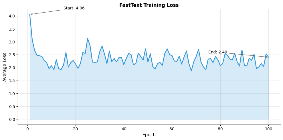
To see FastText in action, we'll train on a small corpus designed to highlight morphological patterns. The corpus contains word families with clear root-suffix relationships: "run/running/runner/runs," "walk/walking/walker/walks," and similar verb conjugations. This controlled setting lets us observe how shared n-grams lead to similar representations:

The model learns from a small corpus with clear morphological patterns. The substantial loss reduction indicates the model successfully learns to distinguish genuine context pairs from negative samples. The n-gram representations allow related word forms to share learned information through common substrings.

To understand what the model learned, let's compare word similarities before and after training:

Handling Out-of-Vocabulary WordsLink Copied

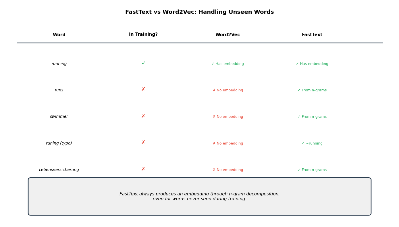
We've arrived at FastText's most compelling feature: the ability to generate meaningful embeddings for words never seen during training. Word2Vec would simply fail when encountering "unfamiliarizing" or "COVID-19" if those terms weren't in its training vocabulary. FastText, by contrast, decomposes any word into n-grams and sums whatever n-gram embeddings it learned during training.

Let's test this capability with a mix of in-vocabulary and out-of-vocabulary words:

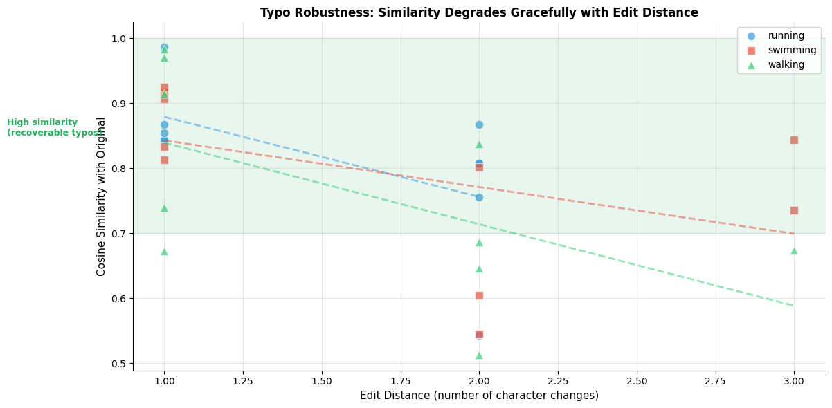
These results reveal FastText's power. Words absent from training (marked with ✗) still receive meaningful embeddings based on their subword structure. "Walked" relates to "walk" and "walker" through shared n-grams like "alk" and "<wa." The intentional typo "runing" correctly associates with "running" because they share most of the same character sequences. Only the doubled "n" differs.

This robustness to OOV words makes FastText particularly valuable for:

• Morphologically rich languages where every possible word form cannot be enumerated
• Domain adaptation where technical terms differ from general vocabulary
• Noisy text where typos and creative spellings are common

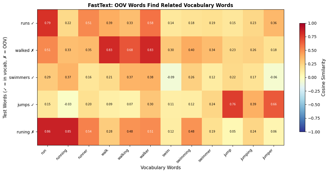
The heatmap reveals that OOV words find their morphological relatives. "Runs" has high similarity with "run," "running," and "runner." "Walked" relates to "walk," "walking," and "walker." Even the typo "runing" correctly associates with "running."

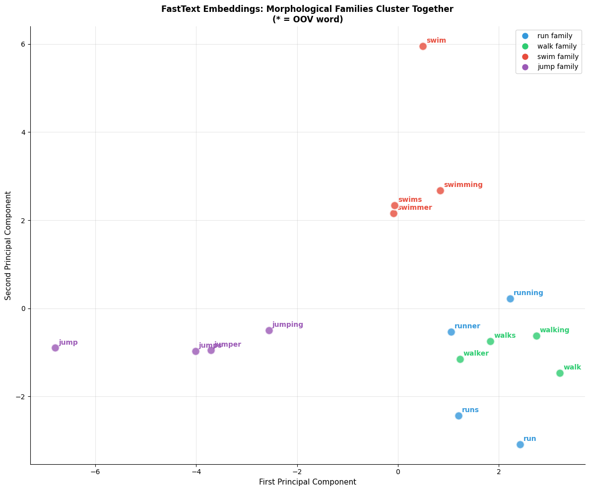
Visualizing the Embedding SpaceLink Copied

Hashing N-grams for Memory EfficiencyLink Copied

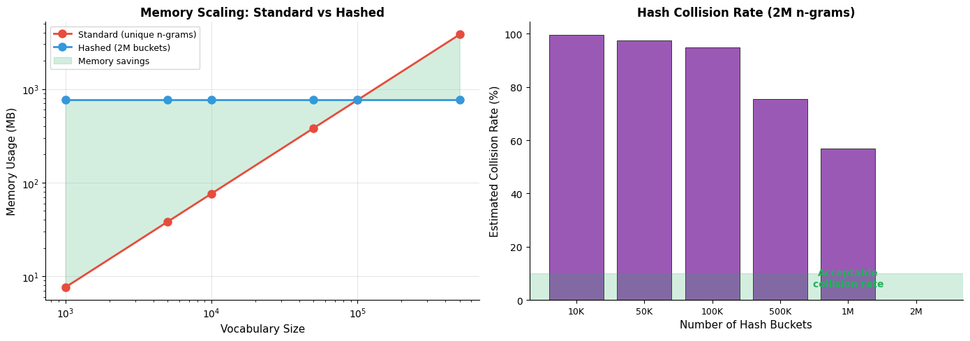
Our implementation so far stores a separate embedding vector for every unique n-gram. This works for toy examples, but scales poorly to real corpora. A vocabulary of 100,000 words with n-gram lengths 3-6 can generate millions of unique n-grams, each requiring a 300-dimensional embedding vector. At 4 bytes per float, this exceeds gigabytes of memory for n-gram embeddings alone.

FastText addresses this through hash-based bucketing: instead of giving each n-gram its own embedding, we hash n-grams to a fixed number of buckets and share embeddings within each bucket.

Even with our small vocabulary, hashing provides meaningful memory savings. The trade-off is that some n-grams will collide to the same bucket and share an embedding, but empirically this has minimal impact on downstream task performance when the number of buckets is sufficiently large.

FastText for Morphologically Rich LanguagesLink Copied

English has relatively simple morphology. Most word variations come from a handful of suffixes like "-ing," "-ed," "-er." But many languages are far more complex. German famously creates compound words by concatenation: "Lebensversicherungsgesellschaft" (life insurance company) combines three roots. Finnish and Turkish use extensive agglutination, where words accumulate suffixes to express grammatical relationships. Arabic and Hebrew have templatic morphology where roots interleave with vowel patterns.

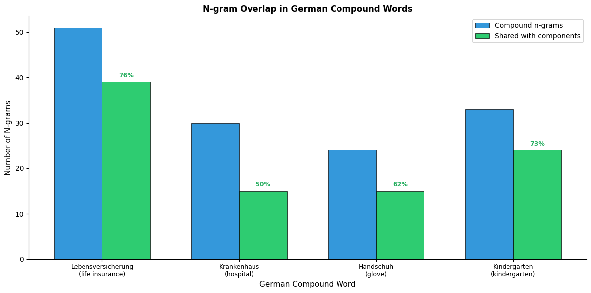
Word2Vec struggles with these languages because the vocabulary explodes. Every possible compound or inflection needs its own embedding. FastText, by contrast, automatically captures the compositional structure through shared n-grams. Let's examine how this works with German compound words:

German compound words share substantial n-gram overlap with their components. "Lebensversicherung" shares n-grams with both "Leben" (life) and "Versicherung" (insurance). This allows FastText to produce meaningful embeddings for unseen compounds based on their constituent parts.

Comparison with Word2VecLink Copied

Let's directly compare FastText and Word2Vec on handling morphological variants and OOV words:

Using Pre-trained FastText ModelsLink Copied

Training FastText from scratch requires substantial computational resources and large corpora. Fortunately, Meta (formerly Facebook) released pre-trained FastText models for 157 languages, trained on Wikipedia and Common Crawl data. These models provide high-quality embeddings out of the box, including the ability to generate vectors for OOV words through their learned n-gram embeddings.

Limitations of FastTextLink Copied

FastText's character n-gram approach solves the OOV problem elegantly, but introduces its own trade-offs. Understanding these limitations helps you decide when FastText is the right tool and when alternatives might serve better.

Static embeddings: Like Word2Vec, FastText produces one embedding per word regardless of context. The word "bank" receives the same vector whether it appears in "river bank" or "bank account." This fundamental limitation, shared by all static embedding methods, motivates the contextual embeddings we'll explore in later chapters.

Character-level noise: The n-gram mechanism has no way to distinguish meaningful subwords from random character sequences. A nonsensical string like "xyzqwk" produces a non-zero embedding through its n-gram components, even though no human would recognize it as a word. This can confuse downstream models that expect zero vectors for unknown tokens.

Memory overhead: Even with hash bucketing, storing embeddings for 2 million n-gram buckets at 300 dimensions requires about 2.4GB in 32-bit floats. Full binary models with word-level embeddings can exceed 7GB, making deployment challenging on memory-constrained devices.

Language-specific assumptions: The n-gram approach assumes that subword character sequences carry meaning. This works beautifully for European languages with alphabetic scripts and productive morphology. But for logographic languages like Chinese (where characters are meaning units, not phonetic components) or languages with complex scripts (Arabic, Devanagari), character n-grams may not capture the right linguistic structure.

Unlike Word2Vec which returns an error for unknown words, FastText always produces an embedding by summing n-gram vectors. While this handles legitimate OOV words well, it means completely meaningless strings also receive embeddings. Applications requiring explicit unknown-word detection need additional logic beyond checking embedding norms.

SummaryLink Copied

FastText extends Word2Vec with a deceptively simple modification that yields profound practical benefits: representing words as bags of character n-grams rather than atomic symbols. This single architectural change, summing n-gram embeddings instead of looking up word embeddings, unlocks capabilities that address Word2Vec's most limiting weakness:

• Out-of-vocabulary handling: Any word, even one never seen during training, receives a meaningful embedding through its subword components
• Morphological awareness: Words sharing the same root naturally cluster together because they share n-grams encoding that root
• Robustness to noise: Typos, creative spellings, and informal text retain most n-grams of their intended words
• Better rare word representations: Rare words benefit from shared n-grams with common words

Key takeaways:

• Subword representation: Words are decomposed into character n-grams (typically lengths 3-6) with boundary markers
• Embedding computation: A word's embedding is the sum of its n-gram embeddings
• Training objective: Same as Word2Vec Skip-gram with negative sampling
• Memory efficiency: Hashing n-grams to fixed buckets reduces memory requirements
• Language coverage: Particularly effective for morphologically rich languages

Despite these improvements, FastText retains Word2Vec's fundamental limitation: each word has exactly one embedding regardless of context. The same vector represents "bank" whether you're discussing finance or fishing. The next chapter examines GloVe, which takes a different approach to the embedding problem: learning from global co-occurrence statistics rather than local context windows. Later chapters will address the context problem directly with models that produce different embeddings for the same word in different sentences.

Key ParametersLink Copied

FastText Parameters:

• min_n (minimum n-gram length): Typically 3. Smaller values capture more context but increase vocabulary size. Setting to 2 captures bigrams like "th" and "ed."

• max_n (maximum n-gram length): Typically 6. Larger values capture longer morphemes but rapidly expand the n-gram vocabulary. For agglutinative languages, consider increasing to 8.

• bucket (number of hash buckets): Typically 2,000,000. Controls memory-quality trade-off. Larger values reduce hash collisions but increase memory usage.

• dim (embedding dimension): Typically 100-300. Higher dimensions capture more nuance but require more data and computation.

• word_ngrams: Whether to include word unigrams in addition to character n-grams. Usually set to 1 (include words).

• epoch: Number of training passes. Typically 5-25. More epochs help with smaller datasets.

• lr (learning rate): Typically 0.05. Higher values speed training but may overshoot. Use learning rate scheduling for best results.

• loss: Training objective. Options include negative sampling (ns), hierarchical softmax (hs), and softmax (softmax). Negative sampling is default and works well for most cases.

• neg (negative samples): Number of negative samples when using negative sampling loss. Typically 5-10. More negatives help with rare words.

• ws (window size): Context window for generating training pairs. Typically 5. Larger windows capture broader semantic relationships.

QuizLink Copied

Ready to test your understanding? Take this quick quiz to reinforce what you've learned about FastText and character n-gram embeddings.