WordPiece Tokenization: BERT's Subword Algorithm Explained

Michael Brenndoerfer

Data, Analytics & AI Machine Learning Language AI Handbook nlp

Master WordPiece tokenization, the algorithm behind BERT that balances vocabulary efficiency with morphological awareness. Learn how likelihood-based merging creates smarter subword units than BPE.

Reading Level

Choose your expertise level to adjust how many terms are explained. Beginners see more tooltips, experts see fewer to maintain reading flow. Hover over underlined terms for instant definitions.

title: "WordPiece Tokenization" format: html: code-fold: false jupyter: python3Link Copied

IntroductionLink Copied

WordPiece is a subword tokenization algorithm that powers BERT and many other transformer-based models. While it shares the iterative merge approach with Byte Pair Encoding (BPE), WordPiece makes a subtle but important change: instead of merging the most frequent pairs, it merges pairs that maximize the likelihood of the training data.

This difference matters. BPE's frequency-based criterion treats all pairs equally regardless of context. A pair appearing 100 times in rare words contributes the same as one appearing 100 times in common words. WordPiece's likelihood objective weights pairs by how much they improve the overall model, giving more influence to patterns that appear in frequent contexts.

The result is a tokenization scheme that tends to produce slightly different vocabularies than BPE, often capturing more linguistically meaningful units. You'll recognize WordPiece tokens by their distinctive ## prefix, which marks subword units that continue a word rather than starting one.

Technical Deep DiveLink Copied

To understand what makes WordPiece different from BPE, we need to think carefully about what it means for a tokenization to be "good." BPE takes a straightforward approach: frequently occurring pairs should become single tokens. But frequency alone misses something important. Consider two pairs that each appear 100 times in a corpus:

Pair A appears in a very common word that occurs 1,000 times
Pair B appears in a rare word that occurs only 100 times

Which pair has a stronger "bond"? Pair B seems more tightly associated: whenever that rare word appears, the pair appears too. Pair A's 100 occurrences represent only 10% of its opportunities. WordPiece captures this intuition by asking not "how often does this pair occur?" but "how often does this pair occur relative to what we'd expect by chance?"

This leads us to a likelihood-based formulation that we'll build up step by step.

Building the Likelihood ModelLink Copied

The foundation is a simple probabilistic model of text. We treat the tokenized corpus as a sequence of independent tokens, each drawn from a probability distribution over the vocabulary. This is called a unigram language model. The term "unigram" reflects that each token is modeled independently, without considering its neighbors.

Given a vocabulary $V$ and a training corpus $C$ tokenized into subword units, the likelihood of the corpus under this model is the product of probabilities for each token:

L(C) = \prod_{i=1}^{n} P(t_i)

where:

$L(C)$ : the likelihood of the corpus, indicating how probable the entire tokenized text is under our model
$n$ : the total number of tokens in the tokenized corpus
$t_i$ : the $i$ -th token in the tokenized corpus
$P(t_i)$ : the probability of token $t_i$ , estimated from the training data

The product arises from the independence assumption: the probability of seeing tokens $t_1, t_2, \ldots, t_n$ in sequence equals $P(t_1) \times P(t_2) \times \cdots \times P(t_n)$ .

How do we estimate each token's probability? The simplest approach is maximum likelihood estimation: count how often each token appears and divide by the total:

P(t) = \frac{\text{count}(t)}{\sum_{t' \in V} \text{count}(t')}

where:

$P(t)$ : the probability assigned to token $t$
$\text{count}(t)$ : the number of times token $t$ appears in the tokenized corpus
$\sum_{t' \in V} \text{count}(t')$ : the total count of all tokens in the vocabulary $V$ , which normalizes the probability

This formula simply says: a token's probability equals its count divided by the total token count, which is the fraction of all tokens that are $t$ . If "the" appears 50,000 times in a corpus of 1,000,000 tokens, then $P(\text{the}) = 0.05$ .

From Likelihood to Merge DecisionsLink Copied

Now comes the key insight. When we merge a pair $(a, b)$ into a new token $ab$ , the likelihood changes. Every occurrence where $a$ and $b$ appeared adjacent is now represented by a single token $ab$ instead of two separate tokens. WordPiece selects the merge that maximizes this likelihood increase.

The key question during training is: which pair of adjacent tokens should we merge next? To answer this, we need to compute how much each possible merge would improve the corpus likelihood. WordPiece does this by computing a score for each candidate pair $(a, b)$ :

\text{score}(a, b) = \frac{\text{count}(ab)}{\text{count}(a) \times \text{count}(b)}

where:

$\text{score}(a, b)$ : the merge priority score for the pair, where higher values mean this pair should be merged sooner
$\text{count}(ab)$ : the number of times tokens $a$ and $b$ appear adjacent to each other in the corpus
$\text{count}(a)$ : the total number of times token $a$ appears in the corpus
$\text{count}(b)$ : the total number of times token $b$ appears in the corpus

This score captures the association strength between tokens $a$ and $b$ . To build intuition, consider what the denominator represents. If tokens appeared randomly and independently throughout the corpus, how often would we expect to see $a$ followed by $b$ ? The product $\text{count}(a) \times \text{count}(b)$ gives a baseline expectation. Dividing the actual co-occurrence count by this baseline measures the "surprise" of seeing them together, quantifying how much more often they appear adjacent than random chance would predict.

A high score means $a$ and $b$ have a strong affinity for each other. They're not just frequent; they're specifically associated. This is exactly what we want in a subword unit.

Pointwise Mutual Information Connection

The WordPiece score is closely related to Pointwise Mutual Information (PMI), a classic measure of association in computational linguistics. PMI measures how much more likely two items appear together compared to if they were independent. The WordPiece score is proportional to the probability ratio that underlies PMI.

Deriving the Score from LikelihoodLink Copied

Let's work through why this score maximizes likelihood. Seeing the derivation helps build deeper understanding.

Step 1: Identify what changes during a merge. When we merge $(a, b)$ into $ab$ :

We remove occurrences of $a$ and $b$ where they appeared as a pair
We add occurrences of the new token $ab$
Occurrences of $a$ and $b$ that weren't adjacent remain unchanged

Step 2: Compute the likelihood ratio. The ratio of the new likelihood to the old likelihood captures the improvement from the merge. For the positions where $(a, b)$ becomes $ab$ , the old likelihood contribution was $P(a) \times P(b)$ for each occurrence, and the new contribution is $P(ab)$ . The likelihood ratio for this merge is proportional to:

\frac{P(ab)^{\text{count}(ab)}}{P(a)^{\text{count}(ab)} \times P(b)^{\text{count}(ab)}}

where:

$P(ab)$ : the probability of the new merged token $ab$ after the merge
$P(a)$ and $P(b)$ : the probabilities of the original tokens before merging
$\text{count}(ab)$ : the number of merge operations (how many times the pair appears)

The exponent $\text{count}(ab)$ appears because each occurrence of the pair contributes independently to the likelihood.

Step 3: Simplify to the score formula. Taking the logarithm converts products to sums and exponents to multiplications, making the expression easier to work with. After simplifying (and noting that the probabilities are proportional to counts), the pair that maximizes the likelihood improvement is the one that maximizes $\frac{\text{count}(ab)}{\text{count}(a) \times \text{count}(b)}$ , which is exactly the WordPiece score.

This derivation reveals that WordPiece's merge criterion isn't arbitrary; it emerges directly from the goal of maximizing data likelihood under a unigram model.

The `##` Prefix NotationLink Copied

WordPiece uses a special notation to distinguish word-initial tokens from continuation tokens. Tokens that continue a word (not at the start) are prefixed with ##.

For example, tokenizing "unhappiness":

un ##happi ##ness

This tells us:

un starts the word
##happi continues from the previous token
##ness continues from the previous token

The ## prefix serves two purposes:

Disambiguation: The token ##ing (word continuation) is different from ing (word start). This matters because "ing" at the start of a word (like "ingot") has different distributional properties than "-ing" as a suffix.
Reconstruction: During decoding, we can easily reconstruct the original text by removing ## prefixes and joining tokens.

The Greedy Tokenization AlgorithmLink Copied

Once we have a trained WordPiece vocabulary, encoding new text follows a greedy longest-match algorithm:

For each word in the input: a. Start at the beginning of the word b. Find the longest token in the vocabulary that matches the current position c. Add that token to the output (with ## prefix if not at word start) d. Move past the matched characters e. Repeat until the word is consumed
If at any point no vocabulary token matches (not even single characters), output the special [UNK] token for the entire word

This greedy approach is fast but not guaranteed to find the globally optimal tokenization. However, it works well in practice and is computationally efficient.

Handling Unknown CharactersLink Copied

Unlike BPE, which typically includes all individual characters in its base vocabulary, WordPiece implementations often have a fixed character set. When encountering characters outside this set:

Character-level fallback: Some implementations add unknown characters to the vocabulary during training
UNK replacement: Others map entire words containing unknown characters to [UNK]
Normalization: Pre-processing can normalize or remove problematic characters

BERT's WordPiece vocabulary, for instance, was trained primarily on English and has limited coverage of characters from other scripts.

Worked ExampleLink Copied

Let's trace through WordPiece training on a small corpus to see how the likelihood-based scoring works.

Consider this training corpus with word frequencies:

"low" (5), "lower" (2), "newest" (6), "widest" (3)

Step 1: Initialization

We start with individual characters (plus the end-of-word marker if used):

Vocabulary: ['d', 'e', 'i', 'l', 'n', 'o', 'r', 's', 't', 'w']

Initial tokenization:

l o w (5)
l o w e r (2)
n e w e s t (6)
w i d e s t (3)

Step 2: Calculate Merge Scores

For each adjacent pair, we calculate the WordPiece score. Recall the formula:

\text{score}(a, b) = \frac{\text{count}(ab)}{\text{count}(a) \times \text{count}(b)}

where $\text{count}(ab)$ is how often $a$ and $b$ appear adjacent, and $\text{count}(a)$ , $\text{count}(b)$ are the total occurrences of each token. Let's compute some scores:

Pair (e, s): appears in "newest" (6) and "widest" (3) = 9 times
- count(e) = 2 + 6 + 3 = 11 (in "lower", "newest", "widest")
- count(s) = 6 + 3 = 9
- score = 9 / (11 × 9) = 0.091
Pair (s, t): appears in "newest" (6) and "widest" (3) = 9 times
- count(s) = 9
- count(t) = 6 + 3 = 9
- score = 9 / (9 × 9) = 0.111
Pair (l, o): appears in "low" (5) and "lower" (2) = 7 times
- count(l) = 5 + 2 = 7
- count(o) = 5 + 2 = 7
- score = 7 / (7 × 7) = 0.143

The pair (l, o) has the highest score, so we merge it first.

Step 3: After First Merge

Vocabulary: ['d', 'e', 'i', 'l', 'lo', 'n', 'o', 'r', 's', 't', 'w']

Updated tokenization:

lo w (5)
lo w e r (2)
n e w e s t (6)
w i d e s t (3)

We continue this process until reaching our target vocabulary size.

Contrast with BPE

With pure frequency counting (BPE), we might merge (e, s) or (s, t) first since they each appear 9 times, compared to (l, o)'s 7 times. The likelihood-based score adjusts for the base frequencies of each token, preferring pairs where the co-occurrence is more "surprising" given the individual token frequencies.

Code ImplementationLink Copied

Let's implement WordPiece from scratch to understand the algorithm deeply. We'll build a simplified version that captures the core concepts.

First, we set up our basic data structures and the scoring function:

In[3]:

Code

from collections import Counter
from typing import Dict, List, Set


class WordPieceTrainer:
    def __init__(self, vocab_size: int = 1000, min_frequency: int = 2):
        self.vocab_size = vocab_size
        self.min_frequency = min_frequency
        self.vocab: Set[str] = set()
        self.word_freqs: Dict[str, int] = {}

    def _get_word_counts(self, corpus: List[str]) -> Dict[str, int]:
        """Count word frequencies in corpus."""
        word_counts = Counter()
        for text in corpus:
            words = text.lower().split()
            word_counts.update(words)
        return dict(word_counts)

    def _tokenize_word(self, word: str) -> List[str]:
        """Tokenize a word into current vocabulary tokens."""
        tokens = []
        start = 0

        while start < len(word):
            end = len(word)
            found = False

            while start < end:
                # Check with ## prefix if not at start
                substr = word[start:end]
                if start > 0:
                    substr = "##" + substr

                if substr in self.vocab:
                    tokens.append(substr)
                    found = True
                    break
                end -= 1

            if not found:
                # Single character fallback
                char = word[start]
                if start > 0:
                    char = "##" + char
                tokens.append(char)
                end = start + 1

            start = end

        return tokens

from collections import Counter
from typing import Dict, List, Set


class WordPieceTrainer:
    def __init__(self, vocab_size: int = 1000, min_frequency: int = 2):
        self.vocab_size = vocab_size
        self.min_frequency = min_frequency
        self.vocab: Set[str] = set()
        self.word_freqs: Dict[str, int] = {}

    def _get_word_counts(self, corpus: List[str]) -> Dict[str, int]:
        """Count word frequencies in corpus."""
        word_counts = Counter()
        for text in corpus:
            words = text.lower().split()
            word_counts.update(words)
        return dict(word_counts)

    def _tokenize_word(self, word: str) -> List[str]:
        """Tokenize a word into current vocabulary tokens."""
        tokens = []
        start = 0

        while start < len(word):
            end = len(word)
            found = False

            while start < end:
                # Check with ## prefix if not at start
                substr = word[start:end]
                if start > 0:
                    substr = "##" + substr

                if substr in self.vocab:
                    tokens.append(substr)
                    found = True
                    break
                end -= 1

            if not found:
                # Single character fallback
                char = word[start]
                if start > 0:
                    char = "##" + char
                tokens.append(char)
                end = start + 1

            start = end

        return tokens

Now let's add the scoring and merge selection logic:

In[4]:

Code

from typing import Tuple


class WordPieceTrainer(WordPieceTrainer):
    def _compute_pair_scores(
        self, splits: Dict[str, List[str]]
    ) -> Dict[Tuple[str, str], float]:
        """Compute WordPiece scores for all adjacent pairs."""
        # Count individual tokens and pairs
        token_counts = Counter()
        pair_counts = Counter()

        for word, freq in self.word_freqs.items():
            tokens = splits[word]
            for token in tokens:
                token_counts[token] += freq
            for i in range(len(tokens) - 1):
                pair = (tokens[i], tokens[i + 1])
                pair_counts[pair] += freq

        # Compute scores
        scores = {}
        for pair, pair_freq in pair_counts.items():
            if pair_freq < self.min_frequency:
                continue
            token_a, token_b = pair
            # WordPiece score: count(ab) / (count(a) * count(b))
            score = pair_freq / (token_counts[token_a] * token_counts[token_b])
            scores[pair] = score

        return scores

    def _merge_pair(
        self, pair: Tuple[str, str], splits: Dict[str, List[str]]
    ) -> Dict[str, List[str]]:
        """Merge a pair of tokens throughout the corpus."""
        token_a, token_b = pair
        # Create merged token (remove ## from second if present)
        if token_b.startswith("##"):
            merged = token_a + token_b[2:]
        else:
            merged = token_a + token_b

        new_splits = {}
        for word, tokens in splits.items():
            new_tokens = []
            i = 0
            while i < len(tokens):
                if (
                    i < len(tokens) - 1
                    and tokens[i] == token_a
                    and tokens[i + 1] == token_b
                ):
                    new_tokens.append(merged)
                    i += 2
                else:
                    new_tokens.append(tokens[i])
                    i += 1
            new_splits[word] = new_tokens

        return new_splits

from typing import Tuple


class WordPieceTrainer(WordPieceTrainer):
    def _compute_pair_scores(
        self, splits: Dict[str, List[str]]
    ) -> Dict[Tuple[str, str], float]:
        """Compute WordPiece scores for all adjacent pairs."""
        # Count individual tokens and pairs
        token_counts = Counter()
        pair_counts = Counter()

        for word, freq in self.word_freqs.items():
            tokens = splits[word]
            for token in tokens:
                token_counts[token] += freq
            for i in range(len(tokens) - 1):
                pair = (tokens[i], tokens[i + 1])
                pair_counts[pair] += freq

        # Compute scores
        scores = {}
        for pair, pair_freq in pair_counts.items():
            if pair_freq < self.min_frequency:
                continue
            token_a, token_b = pair
            # WordPiece score: count(ab) / (count(a) * count(b))
            score = pair_freq / (token_counts[token_a] * token_counts[token_b])
            scores[pair] = score

        return scores

    def _merge_pair(
        self, pair: Tuple[str, str], splits: Dict[str, List[str]]
    ) -> Dict[str, List[str]]:
        """Merge a pair of tokens throughout the corpus."""
        token_a, token_b = pair
        # Create merged token (remove ## from second if present)
        if token_b.startswith("##"):
            merged = token_a + token_b[2:]
        else:
            merged = token_a + token_b

        new_splits = {}
        for word, tokens in splits.items():
            new_tokens = []
            i = 0
            while i < len(tokens):
                if (
                    i < len(tokens) - 1
                    and tokens[i] == token_a
                    and tokens[i + 1] == token_b
                ):
                    new_tokens.append(merged)
                    i += 2
                else:
                    new_tokens.append(tokens[i])
                    i += 1
            new_splits[word] = new_tokens

        return new_splits

Finally, let's add the training loop:

In[5]:

Code

class WordPieceTrainer(WordPieceTrainer):
    def train(self, corpus: List[str]) -> Set[str]:
        """Train WordPiece vocabulary on corpus."""
        # Get word frequencies
        self.word_freqs = self._get_word_counts(corpus)

        # Initialize vocabulary with characters
        all_chars = set()
        for word in self.word_freqs:
            for i, char in enumerate(word):
                if i == 0:
                    all_chars.add(char)
                else:
                    all_chars.add("##" + char)

        self.vocab = all_chars.copy()

        # Initialize splits (each word split into characters)
        splits = {}
        for word in self.word_freqs:
            word_splits = [word[0]]
            for char in word[1:]:
                word_splits.append("##" + char)
            splits[word] = word_splits

        # Iteratively merge pairs
        while len(self.vocab) < self.vocab_size:
            scores = self._compute_pair_scores(splits)

            if not scores:
                break

            # Select best pair
            best_pair = max(scores, key=scores.get)

            # Create merged token
            token_a, token_b = best_pair
            if token_b.startswith("##"):
                merged = token_a + token_b[2:]
            else:
                merged = token_a + token_b

            # Update vocabulary and splits
            self.vocab.add(merged)
            splits = self._merge_pair(best_pair, splits)

        return self.vocab

    def encode(self, text: str) -> List[str]:
        """Encode text using trained vocabulary."""
        words = text.lower().split()
        all_tokens = []

        for word in words:
            tokens = self._tokenize_word(word)
            all_tokens.extend(tokens)

        return all_tokens

    def decode(self, tokens: List[str]) -> str:
        """Decode tokens back to text."""
        result = []
        current_word = []

        for token in tokens:
            if token.startswith("##"):
                current_word.append(token[2:])
            else:
                if current_word:
                    result.append("".join(current_word))
                current_word = [token]

        if current_word:
            result.append("".join(current_word))

        return " ".join(result)

class WordPieceTrainer(WordPieceTrainer):
    def train(self, corpus: List[str]) -> Set[str]:
        """Train WordPiece vocabulary on corpus."""
        # Get word frequencies
        self.word_freqs = self._get_word_counts(corpus)

        # Initialize vocabulary with characters
        all_chars = set()
        for word in self.word_freqs:
            for i, char in enumerate(word):
                if i == 0:
                    all_chars.add(char)
                else:
                    all_chars.add("##" + char)

        self.vocab = all_chars.copy()

        # Initialize splits (each word split into characters)
        splits = {}
        for word in self.word_freqs:
            word_splits = [word[0]]
            for char in word[1:]:
                word_splits.append("##" + char)
            splits[word] = word_splits

        # Iteratively merge pairs
        while len(self.vocab) < self.vocab_size:
            scores = self._compute_pair_scores(splits)

            if not scores:
                break

            # Select best pair
            best_pair = max(scores, key=scores.get)

            # Create merged token
            token_a, token_b = best_pair
            if token_b.startswith("##"):
                merged = token_a + token_b[2:]
            else:
                merged = token_a + token_b

            # Update vocabulary and splits
            self.vocab.add(merged)
            splits = self._merge_pair(best_pair, splits)

        return self.vocab

    def encode(self, text: str) -> List[str]:
        """Encode text using trained vocabulary."""
        words = text.lower().split()
        all_tokens = []

        for word in words:
            tokens = self._tokenize_word(word)
            all_tokens.extend(tokens)

        return all_tokens

    def decode(self, tokens: List[str]) -> str:
        """Decode tokens back to text."""
        result = []
        current_word = []

        for token in tokens:
            if token.startswith("##"):
                current_word.append(token[2:])
            else:
                if current_word:
                    result.append("".join(current_word))
                current_word = [token]

        if current_word:
            result.append("".join(current_word))

        return " ".join(result)

Let's test our implementation:

In[6]:

Code

# Train on a small corpus
corpus = [
    "low low low low low",
    "lower lower",
    "newest newest newest newest newest newest",
    "widest widest widest",
]

trainer = WordPieceTrainer(vocab_size=20, min_frequency=1)
vocab = trainer.train(corpus)

# Train on a small corpus
corpus = [
    "low low low low low",
    "lower lower",
    "newest newest newest newest newest newest",
    "widest widest widest",
]

trainer = WordPieceTrainer(vocab_size=20, min_frequency=1)
vocab = trainer.train(corpus)

Out[7]:

Console

Vocabulary size: 20
Vocabulary: ['##d', '##e', '##er', '##i', '##o', '##r', '##s', '##st', '##t', '##w', 'l', 'lo', 'low', 'lower', 'n', 'ne', 'new', 'w', 'wi', 'wid']

The trained vocabulary contains 20 tokens, including both word-initial characters and merged subword units. Notice how the algorithm has learned tokens like "lo" (from "low"/"lower"), "est" (from "newest"/"widest"), and other common patterns from our corpus.

Now let's test how the trained tokenizer handles various words, including some it hasn't seen before:

In[8]:

Code

# Test encoding on both seen and unseen words
test_words = ["low", "lower", "lowest", "newest", "widest", "newer"]

# Test encoding on both seen and unseen words
test_words = ["low", "lower", "lowest", "newest", "widest", "newer"]

Out[9]:

Console

low        -> ['low']                                  -> low
lower      -> ['lower']                                -> lower
lowest     -> ['low', '##e', '##st']                   -> lowest
newest     -> ['new', '##e', '##st']                   -> newest
widest     -> ['wid', '##e', '##st']                   -> widest
newer      -> ['new', '##er']                          -> newer

The tokenizer successfully handles both training words and novel words like "lowest" and "newer". Words from training ("low", "lower", "newest", "widest") tokenize efficiently using learned subwords. Novel words are decomposed into known subword units. For example, "lowest" uses the learned "lo" and "est" patterns, while "newer" combines "n", "e", "w", "e", "r" since these character-level tokens are in the vocabulary.

Using Hugging Face TokenizersLink Copied

In practice, you'll use optimized implementations like the Hugging Face tokenizers library. Let's see how to train and use a WordPiece tokenizer:

Out[11]:

Console

Vocabulary size: 100

With a vocabulary of 100 tokens trained on our small corpus, the tokenizer has learned common words and subword patterns. Let's test it on some example sentences:

In[12]:

Code

# Test the tokenizer on sample sentences
test_sentences = [
    "machine learning",
    "deep learning models",
    "transformational change",
]

# Test the tokenizer on sample sentences
test_sentences = [
    "machine learning",
    "deep learning models",
    "transformational change",
]

Out[13]:

Console

Input: 'machine learning'
Tokens: ['m', '##a', '##c', '##h', '##in', '##e', 'learn', '##ing']
Decoded: 'm ##a ##c ##h ##in ##e learn ##ing'

Input: 'deep learning models'
Tokens: ['d', '##e', '##e', '##p', 'learn', '##ing', 'm', '##o', '##d', '##e', '##l', '##s']
Decoded: 'd ##e ##e ##p learn ##ing m ##o ##d ##e ##l ##s'

Input: 'transformational change'
Tokens: ['tra', '##n', '##s', '##f', '##or', '##m', '##ation', '##a', '##l', 'c', '##h', '##a', '##n', '##ge']
Decoded: 'tra ##n ##s ##f ##or ##m ##ation ##a ##l c ##h ##a ##n ##ge'

Common words like "machine" and "learning" that appeared frequently in training are kept as whole tokens, while less common words like "transformational" are split into subword units. The ## prefix on continuation tokens allows perfect reconstruction of the original text.

The Hugging Face tokenizer provides a production-ready implementation with special token handling, efficient encoding, and seamless integration with transformer models.

Comparing WordPiece and BPELink Copied

The table below compares how WordPiece and BPE tokenize the same words. Notice the key differences: WordPiece uses the ## prefix to mark continuation tokens, while BPE treats all tokens uniformly. WordPiece also tends to find more morphologically meaningful boundaries.

Tokenization comparison between WordPiece and BPE algorithms. WordPiece uses the##prefix to indicate continuation tokens, making word boundaries explicit.

Word	WordPiece Tokens	BPE Tokens
playing	`play` `##ing`	`play` `ing`
unhappiness	`un` `##happy` `##ness`	`un` `happ` `iness`
internationalization	`inter` `##nation` `##al` `##ization`	`inter` `national` `ization`
transformer	`transform` `##er`	`trans` `former`
embedding	`embed` `##ding`	`emb` `ed` `ding`

The likelihood-based scoring in WordPiece produces different token boundaries than BPE's frequency-based approach. For example, WordPiece keeps "transform" intact as a meaningful unit, while BPE splits it into "trans" and "former". Similarly, WordPiece identifies "happy" as a complete morpheme, while BPE produces "happ" which is less linguistically meaningful.

WordPiece in BERTLink Copied

WordPiece became famous as the tokenization algorithm behind BERT. Understanding how BERT uses WordPiece helps explain its practical impact.

BERT's VocabularyLink Copied

BERT's original English model uses a 30,522 token vocabulary trained on Wikipedia and BookCorpus. The vocabulary includes:

Special tokens: [PAD], [UNK], [CLS], [SEP], [MASK]
Word-initial tokens: Complete words and word prefixes without ##
Continuation tokens: Subword units prefixed with ##

In[14]:

Code

from transformers import BertTokenizer

# Load BERT's tokenizer
bert_tokenizer = BertTokenizer.from_pretrained("bert-base-uncased")
vocab_size = bert_tokenizer.vocab_size

from transformers import BertTokenizer

# Load BERT's tokenizer
bert_tokenizer = BertTokenizer.from_pretrained("bert-base-uncased")
vocab_size = bert_tokenizer.vocab_size

Out[15]:

Console

BERT vocabulary size: 30522

Let's examine how this vocabulary is structured by counting the different token types:

In[16]:

Code

# Examine vocabulary structure
vocab = bert_tokenizer.get_vocab()

# Count token types
continuation_tokens = [t for t in vocab if t.startswith("##")]
special_tokens = ["[PAD]", "[UNK]", "[CLS]", "[SEP]", "[MASK]"]
word_initial_tokens = (
    vocab_size - len(continuation_tokens) - len(special_tokens)
)

# Examine vocabulary structure
vocab = bert_tokenizer.get_vocab()

# Count token types
continuation_tokens = [t for t in vocab if t.startswith("##")]
special_tokens = ["[PAD]", "[UNK]", "[CLS]", "[SEP]", "[MASK]"]
word_initial_tokens = (
    vocab_size - len(continuation_tokens) - len(special_tokens)
)

Out[17]:

Console

Continuation tokens (##): 5828
Word-initial tokens: 24689
Special tokens: 5

The vocabulary splits roughly evenly between word-initial tokens and continuation tokens. This balance allows BERT to represent common words as single tokens while still handling rare or complex words through subword decomposition.

Tokenization in ActionLink Copied

Let's see how BERT tokenizes various text examples:

In[18]:

Code

# Test BERT tokenization on various text examples
test_texts = [
    "Hello world",
    "I love machine learning",
    "Transformers revolutionized NLP",
    "COVID-19 pandemic",
    "antidisestablishmentarianism",
]

# Test BERT tokenization on various text examples
test_texts = [
    "Hello world",
    "I love machine learning",
    "Transformers revolutionized NLP",
    "COVID-19 pandemic",
    "antidisestablishmentarianism",
]

Out[19]:

Console

Text: Hello world
Tokens: ['hello', 'world']
IDs: [7592, 2088]

Text: I love machine learning
Tokens: ['i', 'love', 'machine', 'learning']
IDs: [1045, 2293, 3698, 4083]

Text: Transformers revolutionized NLP
Tokens: ['transformers', 'revolution', '##ized', 'nl', '##p']
IDs: [19081, 4329, 3550, 17953, 2361]

Text: COVID-19 pandemic
Tokens: ['co', '##vid', '-', '19', 'pan', '##de', '##mic']
IDs: [2522, 17258, 1011, 2539, 6090, 3207, 7712]

Text: antidisestablishmentarianism
Tokens: ['anti', '##dis', '##est', '##ab', '##lish', '##ment', '##arian', '##ism']
IDs: [3424, 10521, 4355, 7875, 13602, 3672, 12199, 2964]

Common words like "hello", "world", and "machine" appear as single tokens because they're frequent enough to have their own vocabulary entries. More complex words get decomposed: "revolutionized" splits into "revolution" + "##ized", preserving the morphological structure. The extremely long word "antidisestablishmentarianism" is broken into many subword pieces, but each piece is a meaningful unit that BERT has learned during pre-training.

Handling Special CasesLink Copied

WordPiece in BERT includes several practical handling mechanisms:

In[20]:

Code

# Test special cases: accented characters, non-Latin scripts, numbers, emails
special_cases = [
    "café",  # Accented characters
    "naïve",  # Diacritics
    "北京",  # Chinese characters
    "123.456",  # Numbers
    "user@email.com",  # Email format
]

# Test special cases: accented characters, non-Latin scripts, numbers, emails
special_cases = [
    "café",  # Accented characters
    "naïve",  # Diacritics
    "北京",  # Chinese characters
    "123.456",  # Numbers
    "user@email.com",  # Email format
]

Out[21]:

Console

'café' -> ['cafe']
'naïve' -> ['naive']
'北京' -> ['北', '京']
'123.456' -> ['123', '.', '45', '##6']
'user@email.com' -> ['user', '@', 'email', '.', 'com']

The tokenizer handles accented Latin characters ("café", "naïve") by decomposing them into base characters and accent marks. Numbers and punctuation are also tokenized character-by-character. Chinese characters may produce [UNK] tokens in the English-only BERT model since they weren't in the training vocabulary.

BERT's vocabulary was primarily trained on English text, so it has limited coverage of non-Latin scripts. Multilingual BERT (mBERT) addresses this with a larger vocabulary trained on 104 languages.

Visualization: Token Length DistributionLink Copied

Out[22]:

Visualization

Histogram showing BERT vocabulary token length distribution with separate bars for regular and continuation tokens. — Distribution of token lengths in BERT's WordPiece vocabulary. Most tokens are short (1-4 characters), with a long tail of longer tokens. Continuation tokens (##) average around 3 characters since they capture common suffixes, while word-initial tokens show more variance.

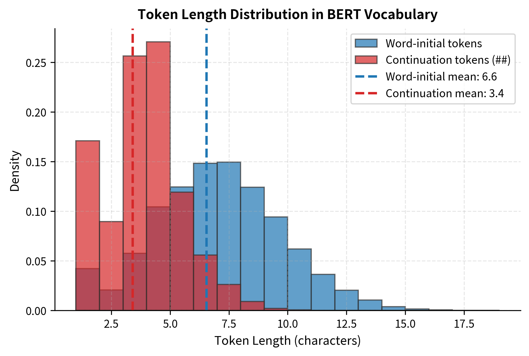
The token length distribution reveals interesting patterns. Continuation tokens (##) tend to be shorter on average because they capture common suffixes like "##ing", "##ed", "##ly". Word-initial tokens include both short function words and longer content words.

Key ParametersLink Copied

The main parameters for WordPiece tokenization are:

vocab_size: The target vocabulary size after training. This controls the trade-off between token granularity and model complexity. BERT uses 30,522 tokens; GPT-2 uses 50,257. Larger vocabularies mean more words are represented as single tokens (reducing sequence lengths), but increase embedding table size. For English-only models, 30,000-50,000 works well. Multilingual models typically use 100,000+ tokens to cover multiple scripts.
min_frequency: Minimum occurrence count for a character pair to be considered for merging during training. Setting this to 2-5 filters out rare patterns that might represent noise. Higher values (5-10) create cleaner vocabularies but may miss useful domain-specific patterns. Lower values (1-2) capture more subword patterns at the risk of overfitting to training corpus idiosyncrasies.
unk_token: The token used to represent out-of-vocabulary characters or words (typically [UNK]). Unlike BPE, which can always fall back to bytes, WordPiece may produce [UNK] tokens for characters not in its vocabulary. This is more common when using a vocabulary trained on a different language or domain.
special_tokens: Reserved tokens with specific roles in the model. Common choices include [CLS] (classification), [SEP] (separator), [PAD] (padding), [MASK] (masked language modeling), and [UNK] (unknown). These are added to the vocabulary before training and excluded from the merge process. Design these based on your model's downstream tasks.

Limitations and ImpactLink Copied

LimitationsLink Copied

WordPiece shares some limitations with BPE:

Context-independent tokenization: The same word always tokenizes the same way regardless of context. "Lead" (the metal) and "lead" (to guide) produce identical tokens, losing the semantic distinction.
Suboptimal for non-Latin scripts: Vocabularies trained primarily on English have poor coverage of other writing systems. Characters from unsupported scripts often become [UNK] tokens.
Greedy encoding: The longest-match encoding algorithm doesn't guarantee globally optimal tokenization. Alternative segmentations might better capture the intended meaning.
Fixed vocabulary: Once trained, the vocabulary can't adapt to new domains without retraining. A model trained on news may struggle with medical text that uses unfamiliar terminology.

ImpactLink Copied

Despite these limitations, WordPiece has been influential:

Enabled BERT's success: The combination of WordPiece tokenization with masked language modeling created one of the most impactful NLP models. BERT's tokenization approach became a template for subsequent models.
Balanced coverage and efficiency: WordPiece's likelihood-based merging creates vocabularies that handle both common and rare words effectively, finding a practical balance between vocabulary size and coverage.
Established subword conventions: The ## prefix notation became widely adopted, providing a clear standard for distinguishing word-initial from continuation tokens.
Inspired improvements: Later algorithms like SentencePiece and Unigram Language Model tokenization built on WordPiece's foundations while addressing some limitations.

SummaryLink Copied

WordPiece tokenization differs from BPE in one crucial way: it selects merges based on likelihood improvement rather than raw frequency. This means pairs that occur more often than expected given their individual frequencies get priority, leading to vocabularies that better capture meaningful subword patterns.

You now understand the key elements of WordPiece:

The likelihood-based scoring formula: $\text{score}(a, b) = \frac{\text{count}(ab)}{\text{count}(a) \times \text{count}(b)}$ , which measures the association strength between adjacent tokens
The ## prefix notation that distinguishes word-initial from continuation tokens
The greedy longest-match encoding algorithm
How BERT applies WordPiece in practice

WordPiece remains a foundational technique in modern NLP, powering BERT and its many variants. While newer tokenization methods have emerged, understanding WordPiece provides essential context for working with transformer models and designing tokenization pipelines.

QuizLink Copied

Ready to test your understanding of WordPiece tokenization? Take this quiz to reinforce the key concepts.

Loading component...

QuizLink Copied

Ready to test your understanding of WordPiece tokenization? Take this quiz to reinforce the key concepts behind BERT's subword algorithm.

Loading component...

Comments

Back to Language AI Handbook

Previous Chapter

Byte Pair Encoding

Next Chapter

Unigram Language Model Tokenization

Reference

BIBTEXAcademic

@misc{wordpiecetokenizationbertssubwordalgorithmexplained, author = {Michael Brenndoerfer}, title = {WordPiece Tokenization: BERT's Subword Algorithm Explained}, year = {2025}, url = {https://mbrenndoerfer.com/writing/wordpiece-tokenization-bert-subword-algorithm}, organization = {mbrenndoerfer.com}, note = {Accessed: 2025-01-01} }

APAAcademic

Michael Brenndoerfer (2025). WordPiece Tokenization: BERT's Subword Algorithm Explained. Retrieved from https://mbrenndoerfer.com/writing/wordpiece-tokenization-bert-subword-algorithm

MLAAcademic

Michael Brenndoerfer. "WordPiece Tokenization: BERT's Subword Algorithm Explained." 2026. Web. today. <https://mbrenndoerfer.com/writing/wordpiece-tokenization-bert-subword-algorithm>.

CHICAGOAcademic

Michael Brenndoerfer. "WordPiece Tokenization: BERT's Subword Algorithm Explained." Accessed today. https://mbrenndoerfer.com/writing/wordpiece-tokenization-bert-subword-algorithm.

HARVARDAcademic

Michael Brenndoerfer (2025) 'WordPiece Tokenization: BERT's Subword Algorithm Explained'. Available at: https://mbrenndoerfer.com/writing/wordpiece-tokenization-bert-subword-algorithm (Accessed: today).

SimpleBasic

Michael Brenndoerfer (2025). WordPiece Tokenization: BERT's Subword Algorithm Explained. https://mbrenndoerfer.com/writing/wordpiece-tokenization-bert-subword-algorithm

Direct link:

https://mbrenndoerfer.com/writing/wordpiece-tokenization-bert-subword-algorithm

About the author: Michael Brenndoerfer

All opinions expressed here are my own and do not reflect the views of my employer.

Michael currently works as an Associate Director of Data Science at EQT Partners in Singapore, leading AI and data initiatives across private capital investments.

With over a decade of experience spanning private equity, management consulting, and software engineering, he specializes in building and scaling analytics capabilities from the ground up. He has published research in leading AI conferences and holds expertise in machine learning, natural language processing, and value creation through data.

View Full Resume Publications Contact Books

WordPiece Tokenization: BERT's Subword Algorithm Explained

title: "WordPiece Tokenization" format: html: code-fold: false jupyter: python3Link Copied

IntroductionLink Copied

Technical Deep DiveLink Copied

Building the Likelihood ModelLink Copied

From Likelihood to Merge DecisionsLink Copied

Deriving the Score from LikelihoodLink Copied

The ## Prefix NotationLink Copied

The Greedy Tokenization AlgorithmLink Copied

Handling Unknown CharactersLink Copied

Worked ExampleLink Copied

Code ImplementationLink Copied

Using Hugging Face TokenizersLink Copied

Comparing WordPiece and BPELink Copied

WordPiece in BERTLink Copied

BERT's VocabularyLink Copied

Tokenization in ActionLink Copied

Handling Special CasesLink Copied

Visualization: Token Length DistributionLink Copied

Key ParametersLink Copied

Limitations and ImpactLink Copied

LimitationsLink Copied

ImpactLink Copied

SummaryLink Copied

QuizLink Copied

QuizLink Copied

Comments

Reference

About the author: Michael Brenndoerfer

Related Content

Unigram Language Model Tokenization: Probabilistic Subword Segmentation

Byte Pair Encoding: Complete Guide to Subword Tokenization

The Vocabulary Problem: Why Word-Level Tokenization Breaks Down

Stay updated

Comments

About the author: Michael Brenndoerfer

Related Content

Unigram Language Model Tokenization: Probabilistic Subword Segmentation

Byte Pair Encoding: Complete Guide to Subword Tokenization

The Vocabulary Problem: Why Word-Level Tokenization Breaks Down

Stay updated

The `##` Prefix NotationLink Copied