

Master Adam optimization with exponential moving averages, bias correction, and per-parameter learning rates. Build Adam from scratch and compare with SGD.

This article is part of the free-to-read Language AI Handbook
Choose your expertise level to adjust how many terms are explained. Beginners see more tooltips, experts see fewer to maintain reading flow. Hover over underlined terms for instant definitions.
Adam Optimizer
Training neural networks requires navigating complex loss landscapes with varying curvature across different parameter dimensions. Some parameters need large updates to escape flat regions, while others need small updates to avoid overshooting sharp valleys. Standard gradient descent treats all parameters equally, using a single learning rate for everything. Momentum helps by smoothing gradients over time, but it still applies the same effective step size everywhere.
Adam, short for Adaptive Moment Estimation, solves this problem by maintaining per-parameter learning rates that automatically adjust based on the history of gradients. It combines two powerful ideas: momentum to smooth gradient direction, and adaptive learning rates to scale step sizes appropriately. Published by Kingma and Ba in 2014, Adam quickly became the default optimizer for deep learning due to its robust performance across architectures and tasks.
This chapter builds Adam from first principles. You'll understand the exponential moving averages that power it, derive the bias correction terms that make it work from the first iteration, and implement Adam from scratch.
Exponential Moving Averages
Adam's core mechanism is the exponential moving average (EMA), a technique for tracking statistics over time while giving more weight to recent observations. Understanding EMA is essential for grasping how Adam adapts to gradient patterns.
An exponential moving average maintains a running estimate that smoothly blends new observations with the historical average. At each step, the estimate is updated as , where controls how much weight goes to the past versus the present.
The update rule is simple:
where:
- : the exponential moving average at time step
- : the previous estimate
- : the new observation at time
- : the decay rate, typically between 0.9 and 0.999
- : the weight assigned to the current observation
The parameter controls the trade-off between stability and responsiveness. High values like create smooth, slowly-changing estimates that ignore short-term fluctuations. Low values like react quickly to new data but can be noisy. The name "exponential" comes from how the influence of past observations decays exponentially with age.
Let's see how the EMA behaves with different decay rates:
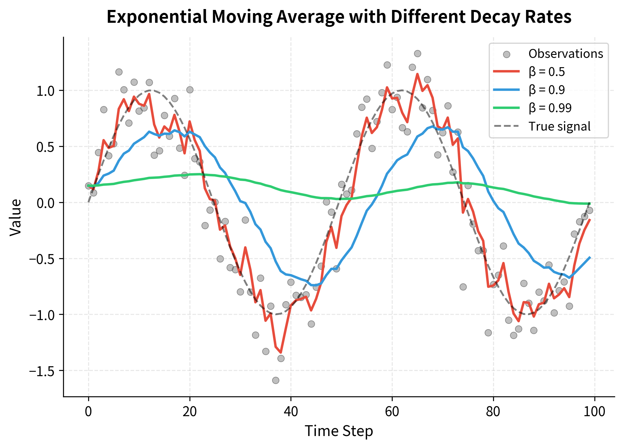
The visualization reveals the trade-off clearly. With , the EMA closely tracks the noisy observations, reacting quickly to changes but inheriting much of the noise. With , the EMA is much smoother but lags significantly behind the true signal. The middle ground of balances responsiveness with stability.
Why Exponential Decay?
To understand why past observations decay exponentially, let's expand the EMA formula recursively. Starting with , we can substitute the formula for :
Distributing the term and continuing this expansion backward to the first observation:
where:
- : the contribution from the current observation (weight )
- : the contribution from the previous observation (weight )
- : the general form for the contribution from observation
- : the residual influence of the initial value (typically zero)
Each observation contributes with weight . Older observations have higher powers of , so their influence decays exponentially. After about time steps, an observation's weight has decayed to roughly of its original value.
The effective memory window determines how many past observations significantly influence the current estimate. To see this decay in action, let's visualize the actual weights assigned to each past observation:
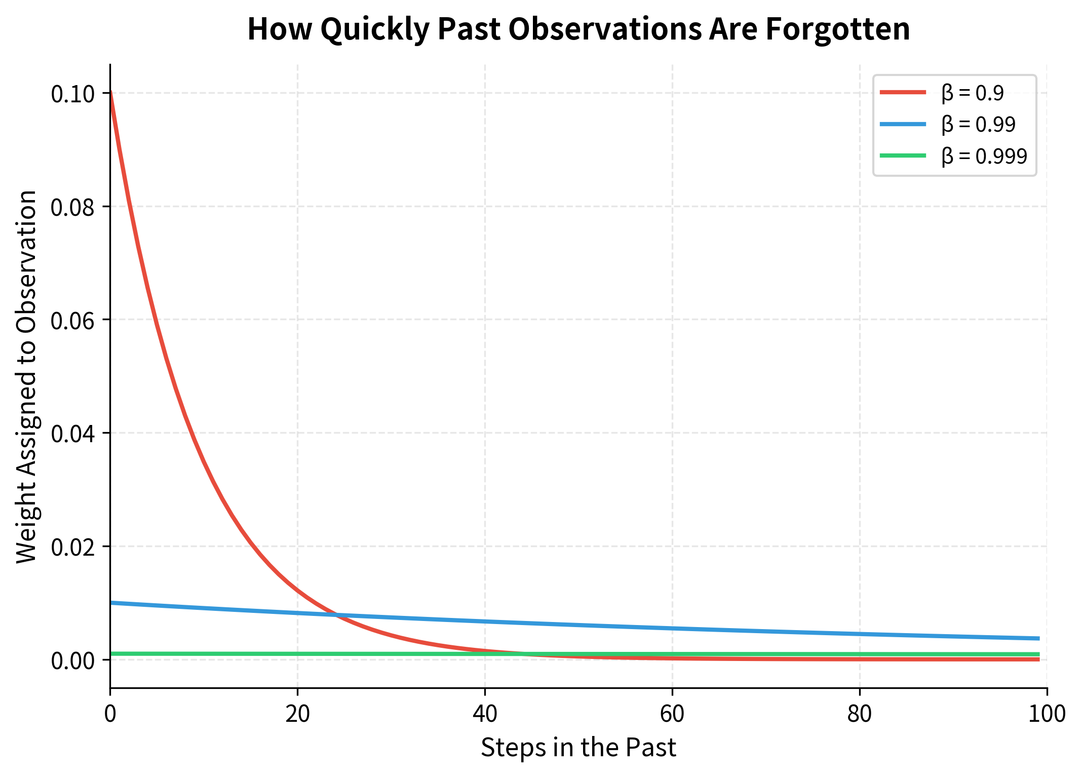
With , the EMA effectively averages over the last 10 observations, making it responsive to recent changes. With , it averages over approximately 1000 observations, providing much greater stability at the cost of slower adaptation. Adam uses these different decay rates for its two moment estimates: for first moment (quick response to gradient direction changes) and for second moment (stable learning rate adaptation).
First Moment: Mean Estimation
Adam tracks two separate exponential moving averages of the gradients. The first moment estimate approximates the mean of recent gradients:
where:
- : the first moment estimate (gradient mean) at step
- : the gradient computed at step
- : the decay rate for the first moment, typically 0.9
This is exactly momentum under a different name. The first moment estimate accumulates a velocity in parameter space, helping the optimizer maintain direction through noisy gradient estimates. When gradients consistently point in the same direction, grows in that direction. When gradients oscillate, dampens the oscillations by averaging out the positive and negative contributions.
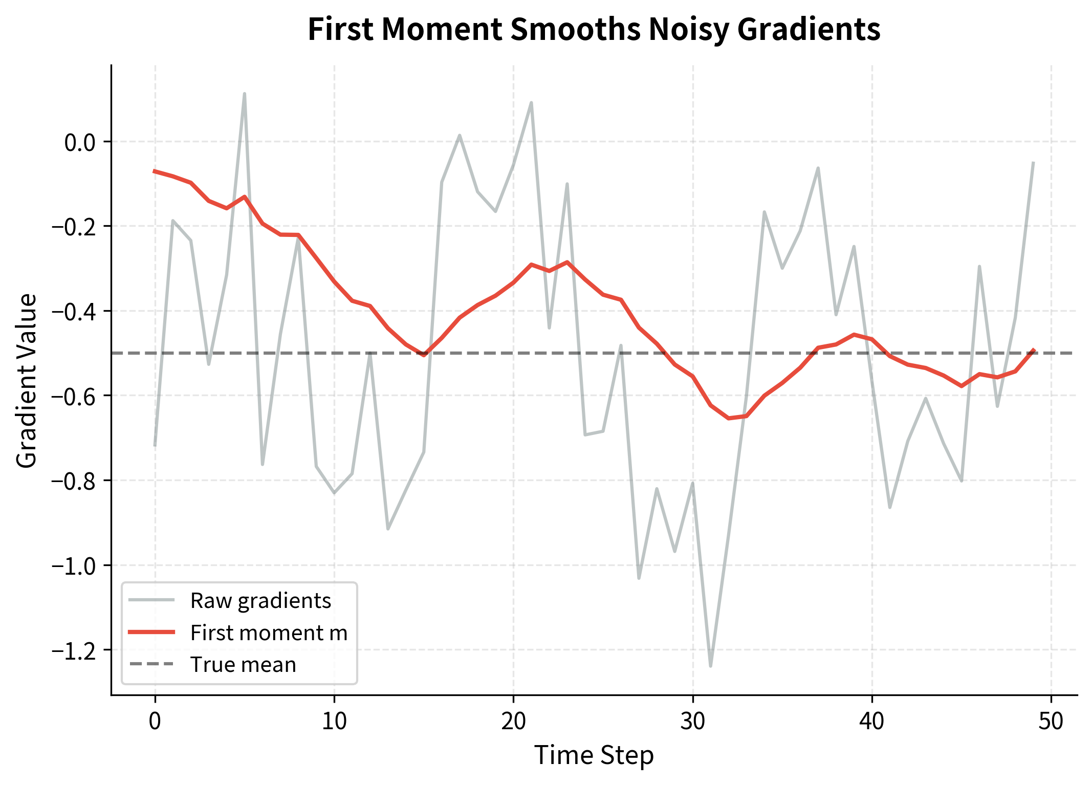
The first moment estimate converges toward the true mean gradient of -0.5, effectively filtering out both the oscillations and the random noise. This momentum effect helps the optimizer move consistently toward the optimum even when individual gradient estimates are unreliable.
First Moment as a Low-Pass Filter
Another way to understand the first moment is as a low-pass filter in signal processing terms. It smooths high-frequency noise while preserving the low-frequency trend. Let's decompose the gradient signal to see this filtering effect:
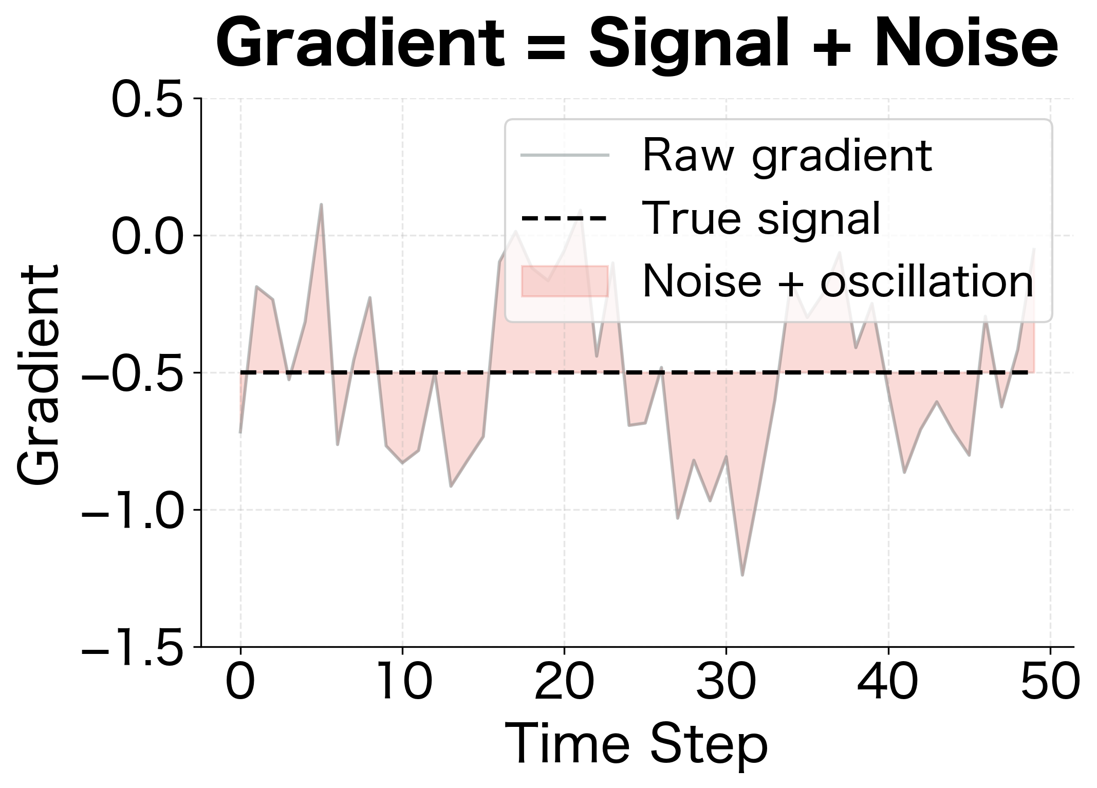
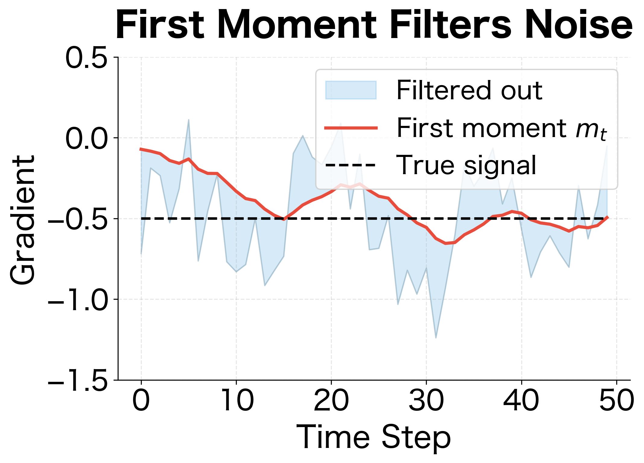
The filtering analogy explains why momentum helps optimization: it extracts the consistent direction from noisy gradient estimates, allowing the optimizer to make confident progress even when individual gradients are unreliable.
Second Moment: Variance Estimation
The second key innovation in Adam is tracking the second moment of gradients, an estimate of their variance. This enables per-parameter learning rate adaptation. The second moment is computed as an EMA of squared gradients:
where:
- : the second moment estimate (uncentered variance) at step
- : the element-wise square of the gradient at step
- : the decay rate for the second moment, typically 0.999
The squared gradients measure how much each parameter's gradient varies over time. Parameters with consistently large gradients will have large values. Parameters with small or sparse gradients will have small values. Adam uses this information to scale learning rates: parameters with high variance get smaller effective learning rates, while parameters with low variance get larger ones.
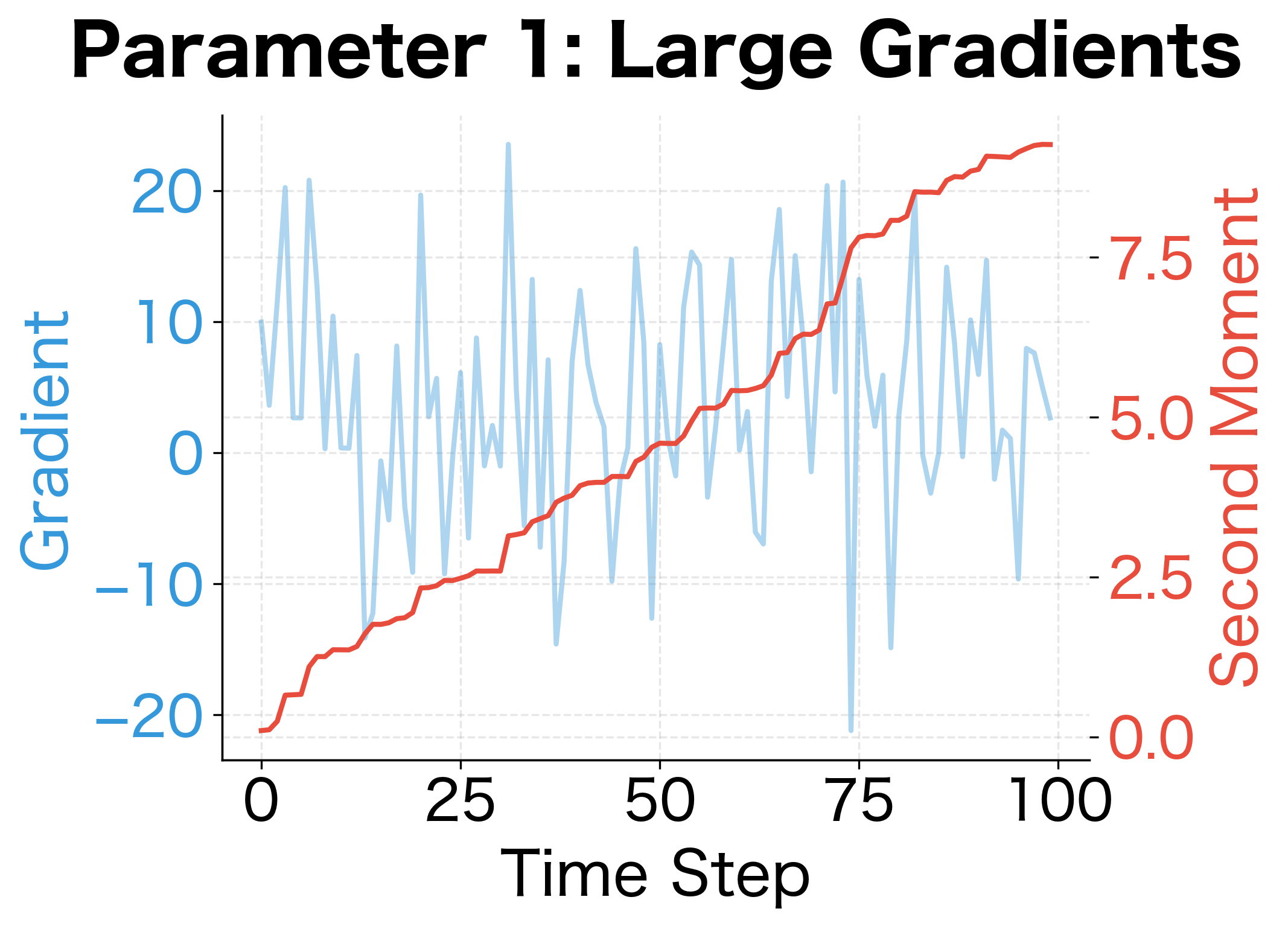
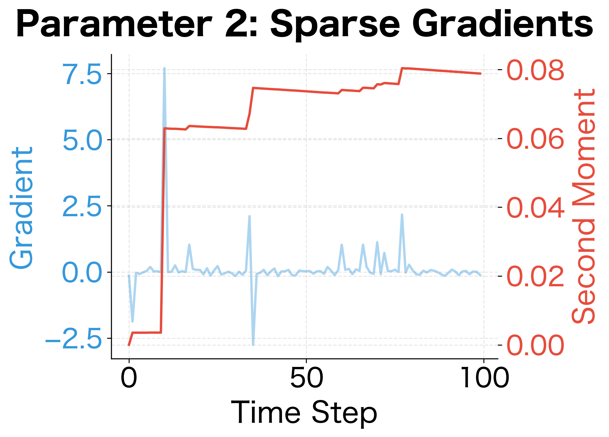
The contrast is striking. Parameter 1's second moment estimate stabilizes around 125 (approximately ), reflecting its consistently large gradients. Parameter 2's second moment remains below 1, reflecting its much smaller typical gradient magnitude. When Adam normalizes updates by , parameter 1 will receive smaller effective steps, while parameter 2 will receive larger ones. This automatic scaling is what makes Adam robust across parameters with very different gradient scales.
The Ratio That Matters
What ultimately determines the effective learning rate is the ratio between the first and second moments. Let's visualize how this ratio differs between our two example parameters:
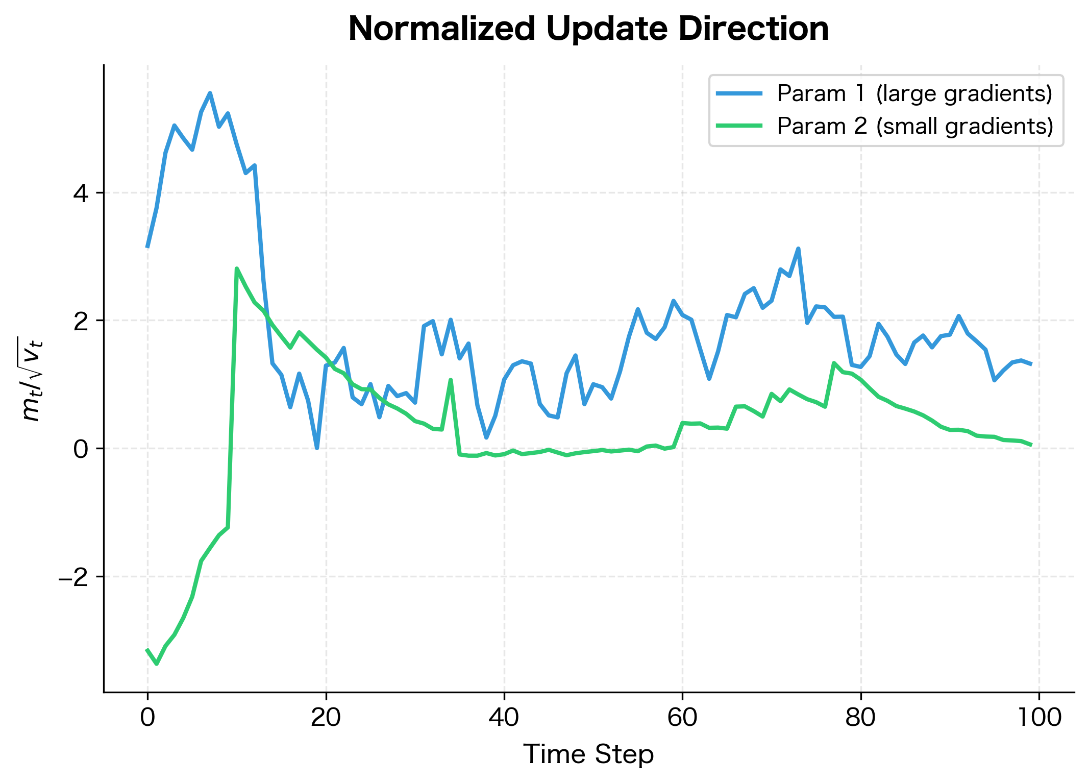
The normalized updates have similar magnitudes despite the 100× difference in raw gradient scales. This is the essence of adaptive learning rates: Adam automatically compensates for gradient scale differences, allowing the same base learning rate to work across diverse parameters.
The Bias Correction Problem
There's a subtle but critical problem with the EMA estimates as we've defined them. At initialization, and . In the first few iterations, the estimates are severely biased toward zero, not because the true gradient mean or variance is near zero, but because the EMA hasn't had time to accumulate information.
To see why this happens, consider the first moment after one step. Starting with , we apply the EMA update:
where:
- : the first moment estimate after one step
- : the contribution from the previous estimate (zero because )
- : the contribution from the current gradient
- : the gradient at step 1
With , we get . The estimate is only 10% of the true gradient! This bias gradually decreases as more observations accumulate, but it takes many steps to fully overcome the zero initialization.
Deriving the Bias Correction
Let's derive the exact bias correction term step by step. We'll show why the biased estimate undershoots and how to correct it.
Step 1: Expand the recurrence relation
Assuming the gradients have true mean (constant over time), we can unroll the EMA recurrence to express as a weighted sum of all past gradients:
where:
- : the weight given to each gradient observation
- : the decay factor for gradient , which depends on how many steps ago it was observed
- The sum runs from (first gradient) to (current gradient)
Step 2: Compute the expected value
Taking the expectation of both sides and using the fact that all gradients have the same expected value :
Step 3: Evaluate the geometric series
The sum is a geometric series. To evaluate it, we substitute to change the indexing. When , we have ; when , we have . This transforms the sum:
The last equality uses the standard geometric series formula: .
Step 4: Derive the bias factor
Substituting the geometric series result back:
The terms cancel, leaving us with a clean expression. The expected value of is not but rather , which is less than since for all finite .
Step 5: Apply the correction
The bias factor is exactly . To get an unbiased estimate, we divide by this factor:
where:
- : the bias-corrected first moment estimate
- : the raw (biased) first moment estimate
- : the correction factor that compensates for zero initialization
The same derivation applies to the second moment:
These bias-corrected estimates converge to the true moments as grows large, since and the correction factor approaches 1.
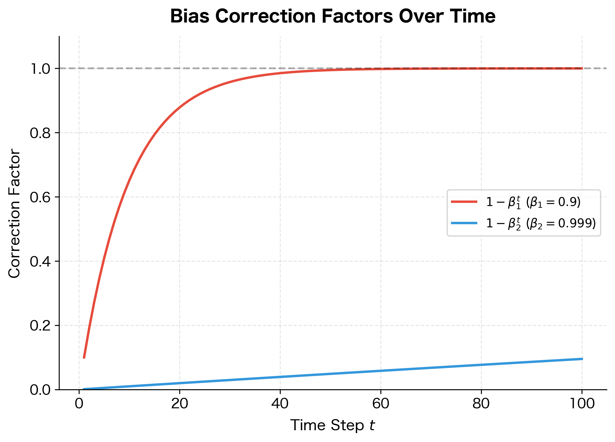
Let's make this concrete with specific values at early time steps:
| Step | (0.9) | Correction | (0.999) | Correction |
|---|---|---|---|---|
| 1 | 0.900 | 0.100 | 0.999 | 0.001 |
| 5 | 0.590 | 0.410 | 0.995 | 0.005 |
| 10 | 0.349 | 0.651 | 0.990 | 0.010 |
| 50 | 0.005 | 0.995 | 0.951 | 0.049 |
| 100 | 0.000 | 1.000 | 0.905 | 0.095 |
| 1000 | 0.000 | 1.000 | 0.368 | 0.632 |
Notice the dramatic difference: dividing by 0.001 at step 1 multiplies the raw second moment by 1000! Without this correction, the effective learning rate would be orders of magnitude too large in early training.
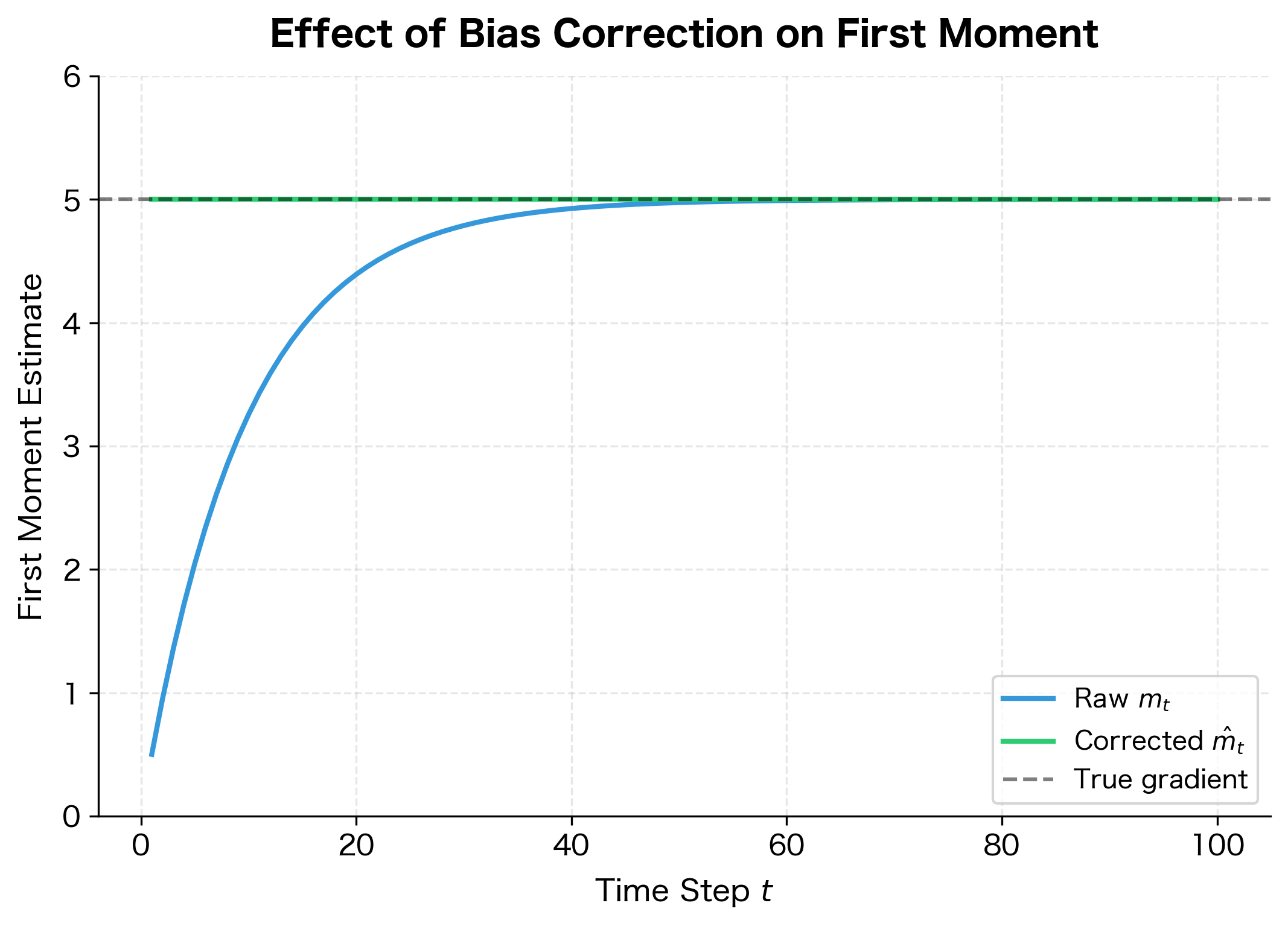
The visualization makes the importance of bias correction clear. Without it, early training steps would use severely underestimated gradients, potentially causing the optimizer to move too slowly or in the wrong direction. With bias correction, Adam produces accurate moment estimates from the very first step.
The Adam Update Rule
We've now developed all the ingredients needed for Adam: exponential moving averages to track gradient statistics, first moment estimates for momentum, second moment estimates for adaptive scaling, and bias correction to handle initialization. The question becomes: how do we combine these pieces into a coherent optimization algorithm?
The key insight is that we want to use the first moment to determine the direction of our update (like momentum), while using the second moment to determine the magnitude of the step for each parameter individually. This combination gives us the best of both worlds: smooth, consistent updates that automatically adapt to each parameter's gradient characteristics.
Building the Update Step by Step
Let's construct the Adam update rule piece by piece, understanding the purpose of each component as we go.
Step 1: Compute the gradient
Every optimization step begins with computing the gradient of the loss function. This tells us which direction would decrease (or increase) the loss for each parameter:
where:
- : the gradient vector at step , containing one value per parameter
- : the gradient operator, which computes partial derivatives with respect to each parameter
- : the loss function evaluated at the current parameter values
The gradient points in the direction of steepest increase in loss. To minimize the loss, we'll move in the opposite direction. But rather than using this gradient directly, we'll first filter it through our moment estimates.
Step 2: Update the first moment estimate
Next, we incorporate the new gradient into our running estimate of the gradient mean. This provides momentum, smoothing out noise and oscillations:
where:
- : the first moment estimate at step
- : the decay rate, typically 0.9, controlling how much we weight past gradients versus the current one
- : the previous first moment estimate
- : the current gradient
Think of as a velocity that accumulates over time. When gradients consistently point in the same direction, the velocity builds up. When gradients oscillate, the velocity averages them out. This is why the first moment provides momentum: it helps the optimizer maintain its trajectory through noisy gradient landscapes.
Step 3: Update the second moment estimate
Simultaneously, we update our estimate of gradient variance by tracking squared gradients:
where:
- : the second moment estimate at step
- : the decay rate, typically 0.999, providing a longer memory than the first moment
- : the previous second moment estimate
- : the element-wise square of the current gradient
The second moment tracks how large gradients tend to be for each parameter. Parameters that consistently receive large gradients will have large values. This information is crucial for adaptive learning rates: we'll use it to shrink the step size for parameters with historically large gradients.
Notice that is larger than (0.999 vs 0.9). This means the second moment has a longer memory, averaging over roughly 1000 recent gradients. The rationale is that the direction we want to move (first moment) should respond quickly to changes, but the scale of how fast to move (second moment) should be more stable.
Step 4: Apply bias correction
Both moment estimates are biased toward zero in early training because they're initialized at zero. We correct this by dividing by the appropriate correction factors:
where:
- : the bias-corrected first moment estimate
- : the bias-corrected second moment estimate
- and : the decay rates raised to the power (the current step number)
- : correction factors that start small and approach 1 as grows
At step , the correction factors are for the first moment and for the second moment. Dividing by these small values amplifies the raw estimates to their unbiased values. As training progresses, approaches zero, the correction factors approach 1, and the correction becomes negligible.
Step 5: Update the parameters
Finally, we combine the bias-corrected moments into the parameter update:
where:
- : the updated model parameters
- : the parameters before this step
- : the learning rate, a hyperparameter controlling overall step size
- : the bias-corrected first moment, determining the update direction
- : the square root of the bias-corrected second moment, scaling each parameter's step size
- : a small constant (typically ) preventing division by zero
This is the heart of Adam. The numerator provides a momentum-smoothed gradient direction. The denominator scales each parameter's update inversely to its typical gradient magnitude. Parameters with large historical gradients get smaller steps; parameters with small historical gradients get larger steps.
The division is element-wise, so each parameter receives its own personalized learning rate. This is fundamentally different from SGD or momentum, which apply the same learning rate to all parameters.
Why This Formula Works
To understand why Adam's update rule is effective, consider what happens to the effective learning rate for each parameter. The effective learning rate for parameter at step is:
where:
- : the effective learning rate for parameter at step
- : the base learning rate specified by the user
- : the bias-corrected second moment for parameter
- : the numerical stability constant
This formula reveals Adam's adaptive behavior:
-
Large gradients → small effective learning rate: When gradients for parameter are consistently large, grows, and the denominator increases. This shrinks the effective learning rate, preventing the optimizer from taking steps that are too large.
-
Small gradients → large effective learning rate: When gradients are consistently small, stays small, keeping the denominator near . The effective learning rate remains close to , allowing the optimizer to take meaningful steps even when gradients are tiny.
-
Variable gradients → intermediate behavior: Parameters with fluctuating gradient magnitudes get intermediate effective learning rates that adapt as the training dynamics evolve.
This adaptive behavior has several practical benefits:
-
Scale invariance: If we rescale the gradients for a parameter by a constant factor , both the numerator and denominator scale proportionally, leaving the update direction unchanged. This makes Adam less sensitive to how features are scaled.
-
Robustness across architectures: Different layers in a neural network often have very different gradient magnitudes. Embedding layers might have sparse, large gradients while output layers have dense, small gradients. Adam automatically adjusts for these differences.
-
Handling sparse gradients: In NLP models with large vocabularies, most word embeddings receive zero gradients on any given batch. When a word does appear, Adam gives it a larger update because its second moment is small. This helps rare words learn effectively.
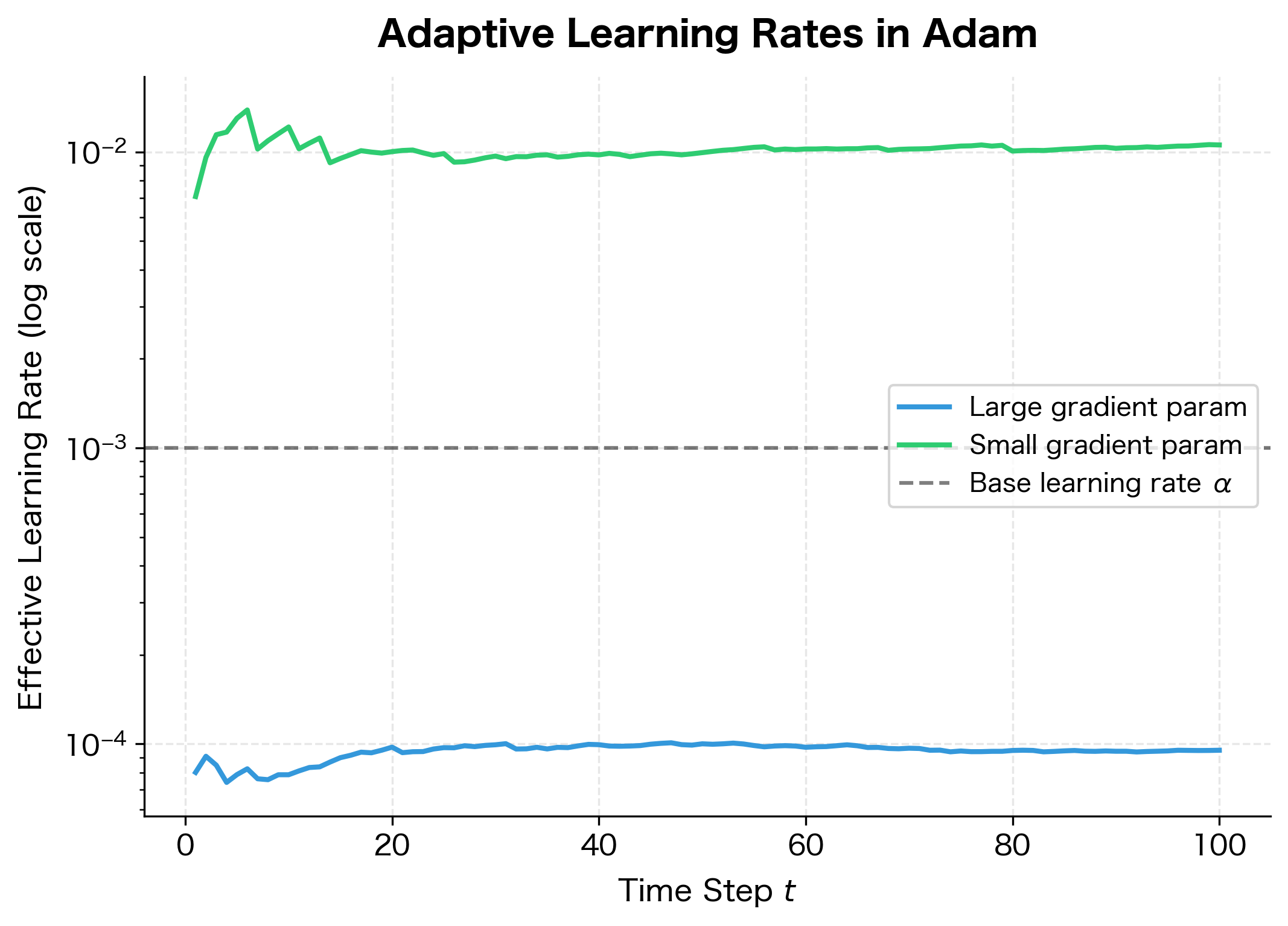
The difference in effective learning rates spans orders of magnitude. The parameter with large gradients ends up with an effective learning rate around , while the parameter with small gradients retains a rate close to . This automatic adaptation is why Adam often works well "out of the box" without extensive learning rate tuning.
Visualizing the Complete Update
To see how all the pieces fit together, let's trace through a single Adam update step, showing how the gradient flows through each transformation:
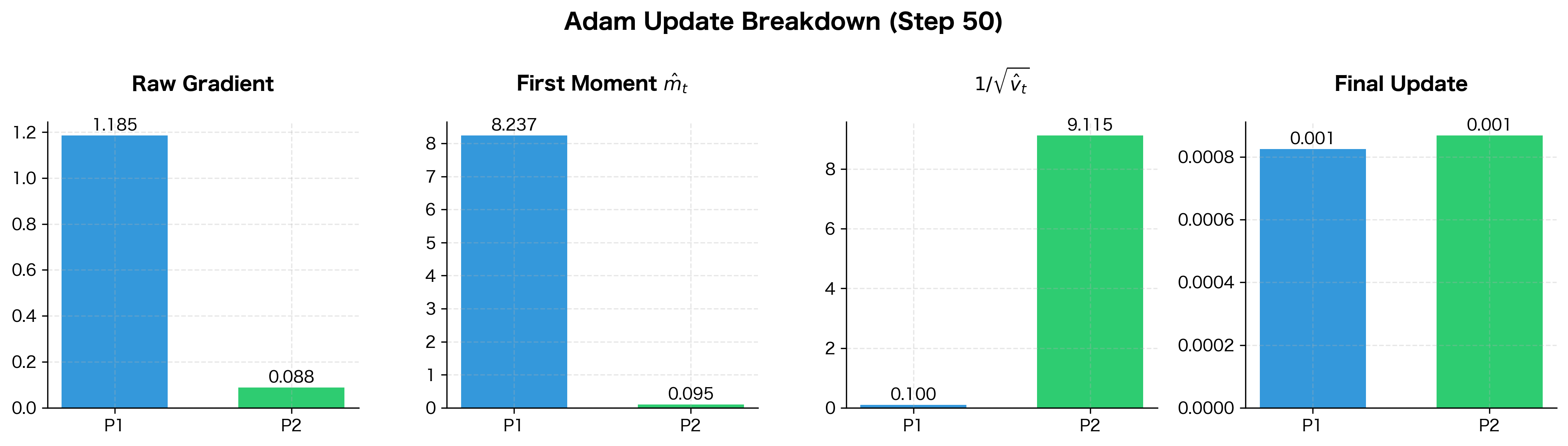
The breakdown reveals Adam's balancing act. Parameter 1 has a raw gradient ~100× larger than Parameter 2, but its inverse scaling factor is correspondingly smaller. The final updates end up much closer in magnitude than the raw gradients, ensuring both parameters make meaningful progress without destabilizing the optimization.
Implementing Adam from Scratch
With the theory in place, let's translate the Adam algorithm into code. Building an optimizer from scratch solidifies understanding and reveals the elegance of the approach. We'll then test our implementation on a challenging optimization problem to see Adam in action.
The Adam Class
Our implementation needs to track several pieces of state:
- The parameters being optimized
- The hyperparameters (, , , )
- The first and second moment estimates for each parameter
- The current time step for bias correction
Here's a clean implementation that mirrors the mathematical formulation:
The implementation is compact. The __init__ method sets up the hyperparameters and initializes the moment estimates to zero. The step method implements exactly the five steps we derived: it updates both moment estimates, applies bias correction, and computes the parameter update.
Notice that the parameters are modified in-place (param -= ...). This is a common pattern in optimization: the optimizer receives references to the actual parameter arrays and modifies them directly. The caller doesn't need to extract updated values from the optimizer.
Testing on the Rosenbrock Function
To see Adam in action, we'll minimize the Rosenbrock function, a classic benchmark that has tormented optimizers since 1960. The function is defined as:
The global minimum is at where . What makes this function challenging is its shape: a long, narrow, curved valley where the gradient points mostly across the valley rather than along it toward the minimum. Simple gradient descent tends to oscillate across the valley while making slow progress along it.
Let's define the function and its gradient, then optimize from a starting point of :
Adam converges to the optimum with impressive precision. The distance to the true minimum is on the order of , and the final loss is near machine precision. This demonstrates that Adam's adaptive learning rates successfully navigate the challenging curved valley structure.
Visualizing the Optimization Trajectory
To understand how Adam navigates the Rosenbrock landscape, let's visualize both the trajectory through parameter space and the loss curve over time:
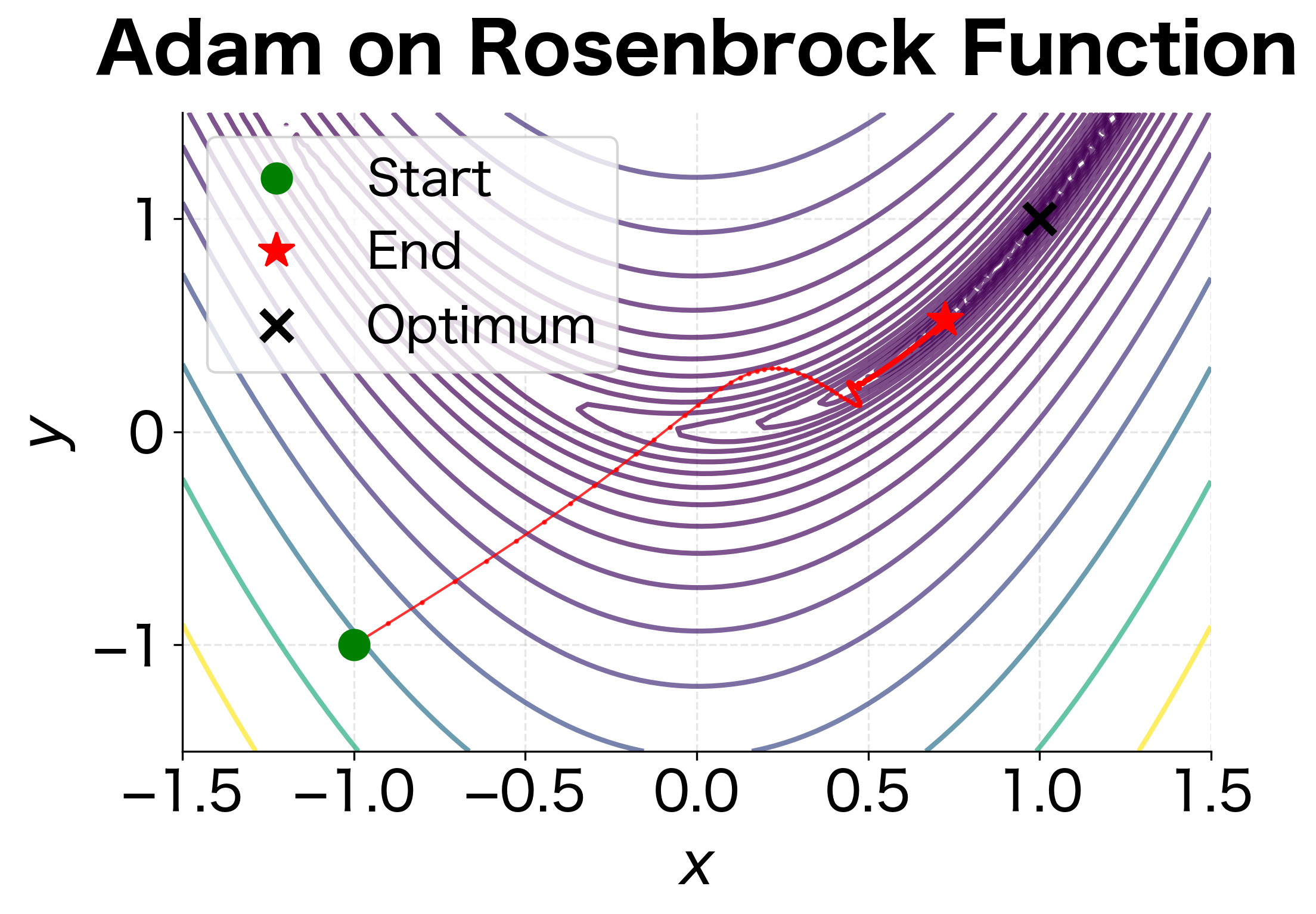
The trajectory reveals Adam's strategy. Rather than oscillating across the narrow valley like simple gradient descent would, Adam quickly finds the valley floor and then follows it toward the minimum. The adaptive learning rates are essential here: the direction has much steeper curvature than the direction, and Adam automatically uses different step sizes for each.
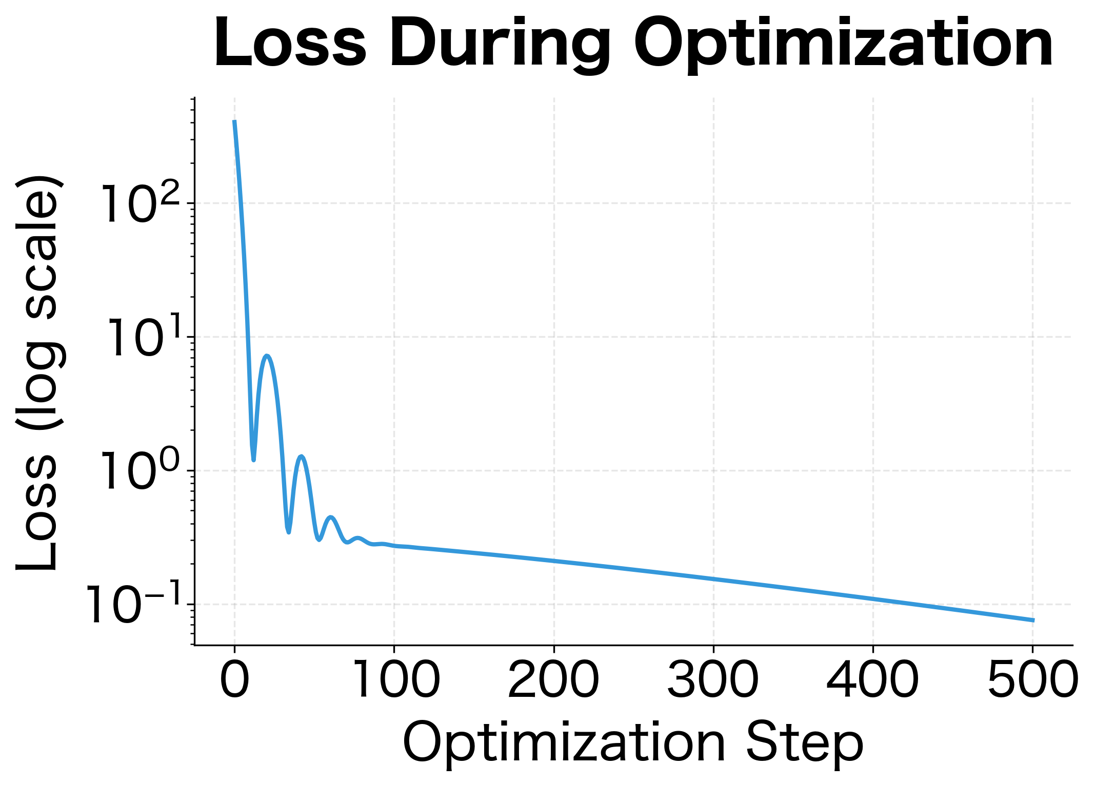
The loss curve shows characteristic behavior. There's an initial rapid decrease as Adam approaches the valley, followed by slower but steady progress along the valley floor. The log scale reveals that Adam continues making progress even when the loss appears to plateau on a linear scale.
Comparing with SGD and Momentum
How does Adam compare to simpler optimizers? Let's benchmark against SGD and SGD with momentum on the same problem:
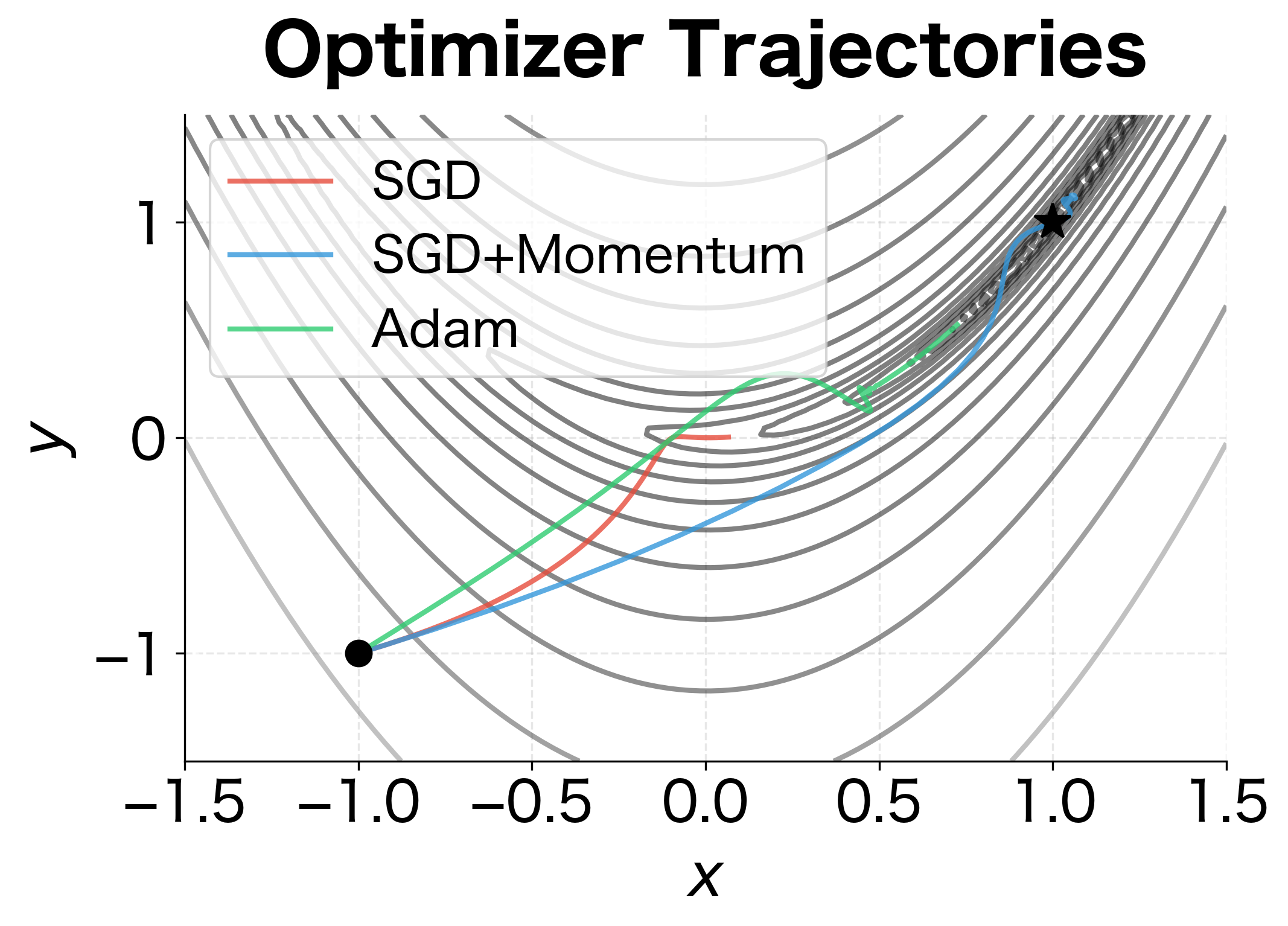
The comparison reveals Adam's advantages. With comparable learning rates, SGD would barely move because it can't handle the different scales across the two dimensions. With a larger learning rate, it would oscillate wildly. Momentum helps by building up velocity in consistent directions, but it still struggles with the changing curvature. Adam's per-parameter adaptation allows it to use a much larger effective learning rate while maintaining stability.
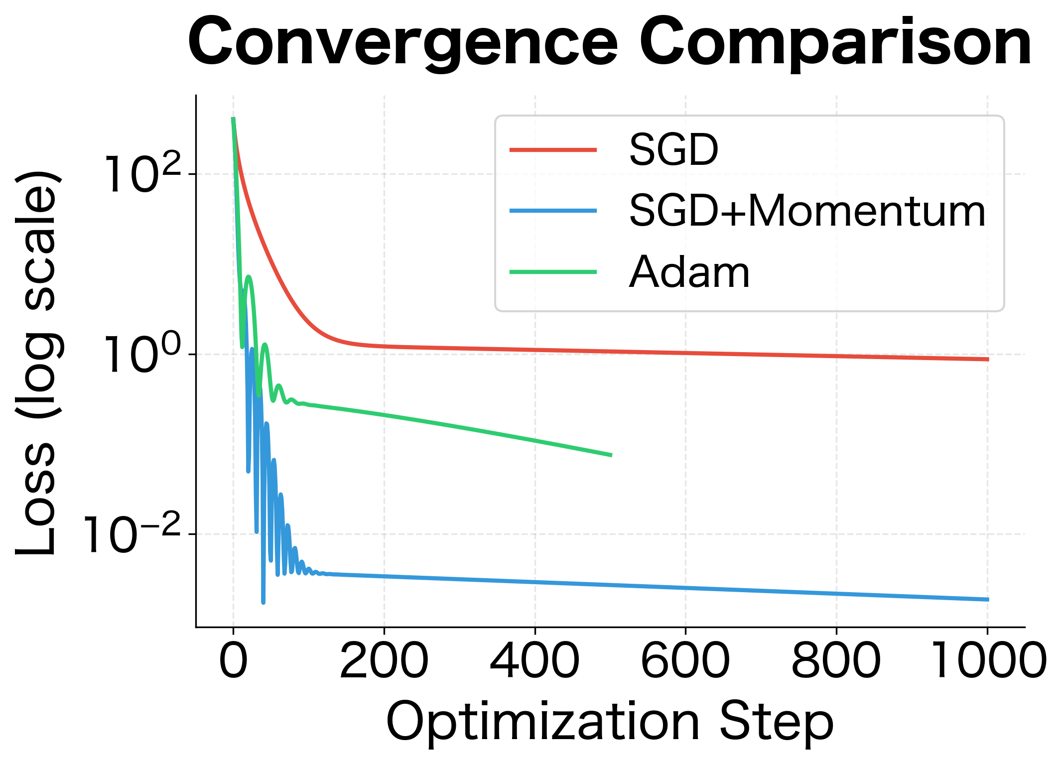
Quantifying the Difference
Let's measure the concrete performance difference between optimizers:
Adam achieves orders of magnitude better convergence in half the iterations. The adaptive learning rates allow it to use an effective step size 1000× larger than what SGD can safely handle, accelerating progress through the curved valley.
Adam Hyperparameters
Adam has four hyperparameters, but in practice only the learning rate usually requires tuning. The default values work well for most problems.
Learning rate (): The most important hyperparameter. Common values range from 0.0001 to 0.01, with 0.001 as a typical starting point for deep learning. Unlike SGD, Adam is relatively robust to learning rate choice due to its adaptive scaling, but extreme values can still cause problems. Too high leads to instability; too low leads to slow convergence.
First moment decay (): Controls momentum. The default value of 0.9 works well for most problems. Lower values (0.8) reduce momentum and make the optimizer more responsive to recent gradients. Higher values (0.95, 0.99) increase smoothing but may slow adaptation to changing loss landscapes. For problems with very noisy gradients, consider increasing .
Second moment decay (): Controls the learning rate adaptation timescale. The default of 0.999 provides stable second moment estimates. Lower values (0.99, 0.9) adapt learning rates more quickly but can be unstable. For sparse gradient problems (like NLP with large vocabularies), the default 0.999 is usually appropriate.
Epsilon (): Numerical stability constant. The default is almost always fine. Some frameworks use or . Larger values add a minimum "floor" to the effective learning rate, which can help when second moments become very small.
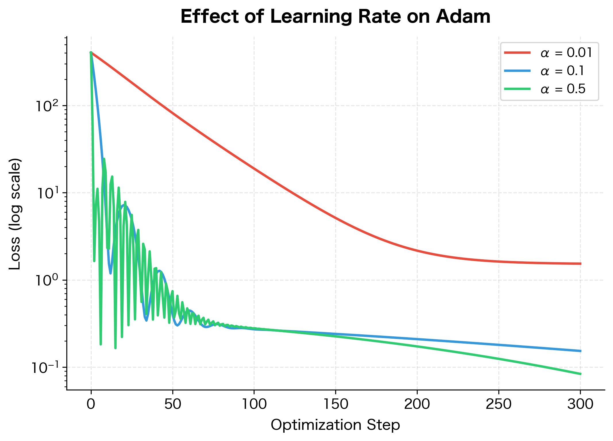
The learning rate of 0.1 achieves the fastest convergence and lowest final loss, while 0.01 converges more slowly but steadily. The highest rate of 0.5 may introduce instability depending on the problem. For most deep learning tasks, starting with 0.001 and adjusting based on training dynamics is a practical approach.
Effect of β₁ on Momentum
While the learning rate is the primary tuning knob, β₁ controls how much the optimizer relies on past gradients versus the current one. Let's visualize this trade-off:
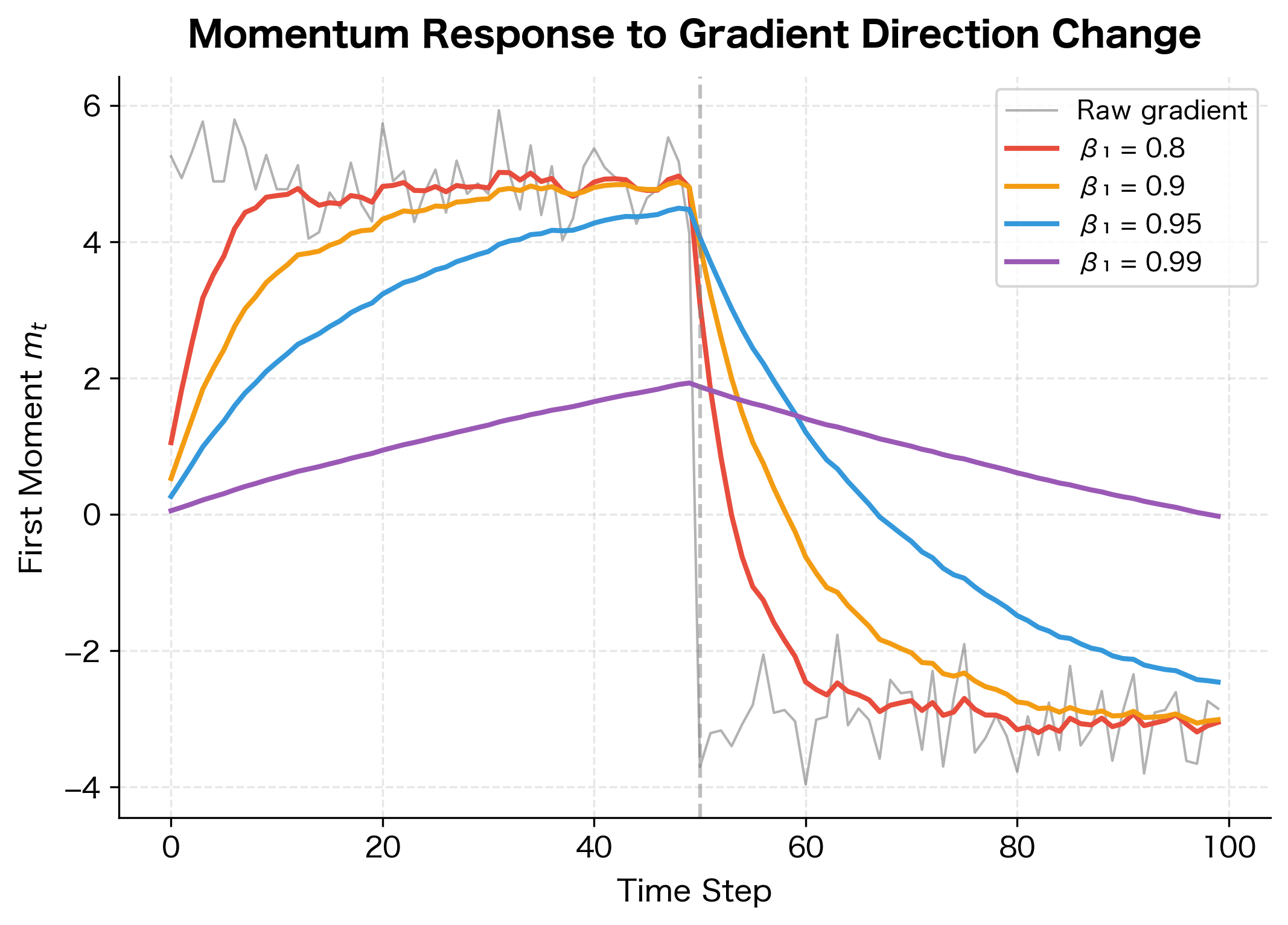
When the gradient direction changes abruptly at step 50, lower β₁ values adapt within a few steps while higher values take tens of steps to reverse direction. For training scenarios with non-stationary objectives (like curriculum learning), consider reducing β₁ for faster adaptation.
Convergence Properties
Adam's theoretical convergence properties have been studied extensively. Under certain conditions (convex loss, bounded gradients, appropriate learning rate decay), Adam converges to the optimum. However, several practical considerations affect real-world performance.
When Adam Excels
Adam performs particularly well in several scenarios:
- Sparse gradients: NLP models with large vocabularies, where most embedding gradients are zero on any given batch
- Non-stationary objectives: Training with data augmentation or curriculum learning where the effective loss changes over time
- Noisy gradients: Small batch sizes where gradient estimates have high variance
- Different parameter scales: Models combining embeddings, convolutions, and dense layers with very different gradient magnitudes
Known Issues
Adam has some documented failure modes:
- Poor generalization: Empirically, Adam sometimes generalizes worse than SGD with momentum on image classification, possibly due to converging to sharper minima
- Weight decay interaction: Standard L2 regularization doesn't work correctly with Adam due to the adaptive learning rates (this motivates AdamW, covered in the next chapter)
- Non-convergence cases: Reddi et al. (2018) showed examples where Adam fails to converge, leading to AMSGrad, a variant that maintains maximum second moments
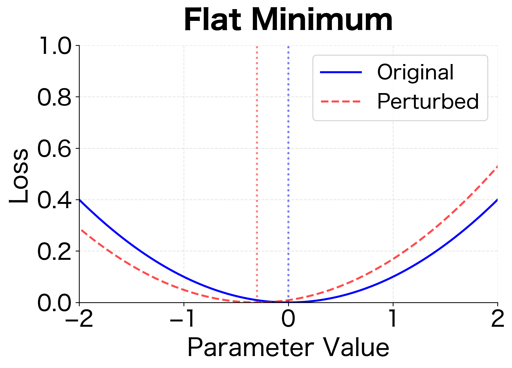
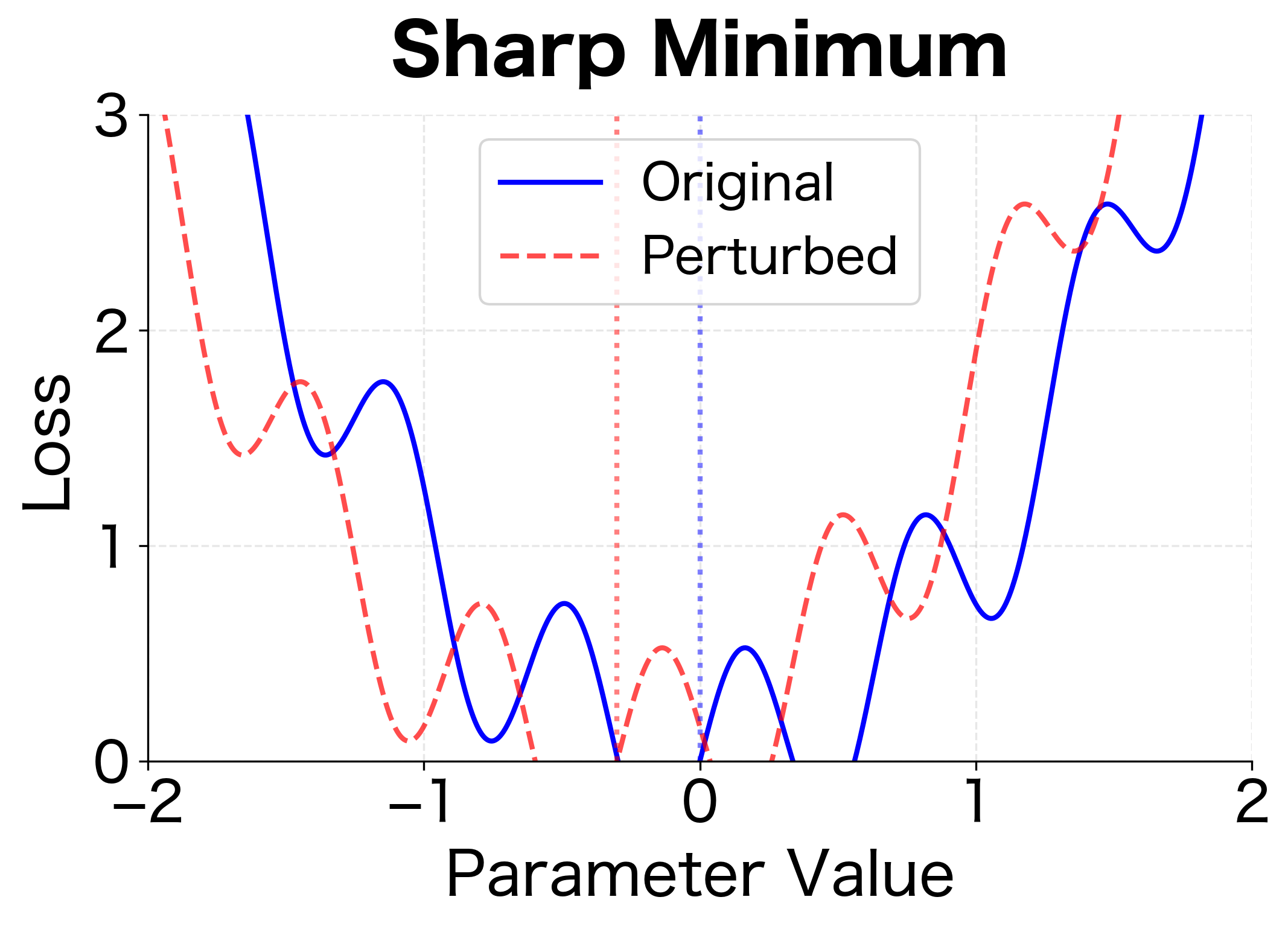
The flat vs. sharp minimum distinction matters for generalization. Test data comes from a slightly different distribution than training data, analogous to the perturbation in the figure. Models that find flat minima are more robust to this distribution shift.
Using Adam in PyTorch
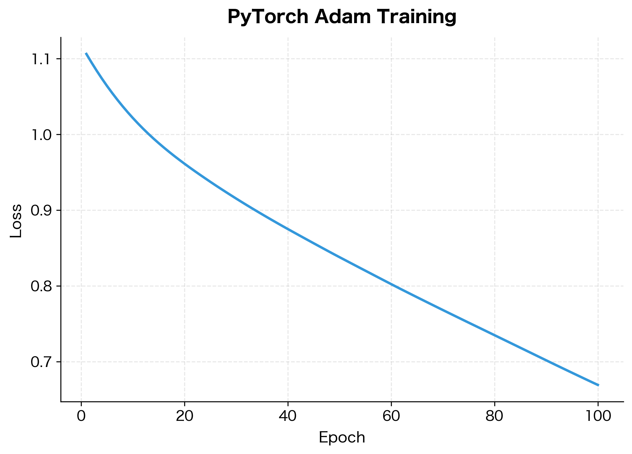
In practice, you'll use framework implementations. PyTorch's Adam is highly optimized and handles all the bookkeeping automatically:
The network reduces its loss substantially over 100 epochs. The improvement percentage shows how much the model has learned from the synthetic data. In practice, you would monitor both training and validation loss to detect overfitting.
Inspecting Optimizer State
One advantage of PyTorch is easy access to the optimizer's internal state. Let's examine the moment estimates for different layers:
The state reveals interesting patterns. Weights and biases have different moment statistics, reflecting their different gradient characteristics during training. The first layer (fc1) and second layer (fc2) also show distinct patterns, demonstrating how Adam maintains per-parameter adaptation throughout the network.
PyTorch's implementation includes several optimizations beyond our simple version, including fused CUDA kernels for GPU training and memory-efficient gradient handling. For production use, always prefer the framework implementation.
Limitations and Practical Considerations
While Adam is effective, it isn't perfect. Understanding its limitations helps you know when to consider alternatives.
The most significant practical issue is Adam's interaction with weight decay regularization. Standard L2 regularization adds a term to the loss, which adds to the gradient, where is the regularization strength and represents the model parameters. But Adam's adaptive learning rates interfere with this: parameters with large gradients have large second moments , which reduces their effective learning rate. This means the regularization gradient is also scaled down, so parameters with large gradients effectively receive less regularization. This motivated the development of AdamW, which decouples weight decay from the gradient computation.
Another limitation is memory usage. Adam stores two additional values (first and second moments) per parameter, tripling memory requirements compared to SGD. For very large models, this can be a significant constraint. Optimizers like Adafactor address this by factorizing the moment matrices.
Adam's default hyperparameters work well across many problems, but they aren't universally optimal. For some tasks, especially those where SGD ultimately achieves better generalization, Adam may converge quickly to a suboptimal solution. In these cases, practitioners sometimes use Adam for initial rapid progress, then switch to SGD for fine-tuning.
Key Parameters
When using Adam in practice, these are the parameters you'll encounter most frequently:
lr (learning rate, ): Controls the overall step size. Start with 0.001 for most deep learning tasks. Increase to 0.01 for faster initial convergence on simpler problems, or decrease to 0.0001 for fine-tuning pretrained models. This is the only hyperparameter that typically requires tuning.
betas (momentum coefficients): A tuple of controlling the decay rates for first and second moment estimates. The defaults (0.9, 0.999) work well for most problems. Consider increasing to 0.95 for very noisy gradients, or decreasing to 0.99 for sparse gradient scenarios.
eps (epsilon): Numerical stability constant added to the denominator. The default of is appropriate for most cases. Increase to or if you observe numerical instability with very small second moments.
weight_decay: In standard Adam, this applies L2 regularization through the gradient (not recommended). For proper weight decay, use AdamW instead, which decouples the regularization from the adaptive learning rate mechanism.
Summary
Adam combines momentum and adaptive learning rates into a single, robust optimizer. By tracking exponential moving averages of gradients (first moment) and squared gradients (second moment), it automatically scales updates for each parameter based on its gradient history.
Key takeaways from this chapter:
- Exponential moving averages smooth noisy signals by blending new observations with historical estimates, with the decay rate controlling the trade-off between stability and responsiveness
- First moment estimation () provides momentum, accumulating velocity in consistent gradient directions
- Second moment estimation () tracks gradient variance, enabling per-parameter learning rate adaptation
- Bias correction compensates for zero initialization, ensuring accurate moment estimates from the first step
- The Adam update divides the bias-corrected first moment by the square root of the bias-corrected second moment, naturally scaling step sizes
- Hyperparameters include learning rate (, typically 0.001), first moment decay (, typically 0.9), second moment decay (, typically 0.999), and numerical stability constant (, typically )
- Adaptive learning rates make Adam robust across parameters with different gradient scales, often working well without extensive tuning
Adam's practical success made it the default optimizer for much of deep learning. However, its interaction with weight decay regularization led to the development of AdamW, which we'll explore in the next chapter.
Quiz
Ready to test your understanding? Take this quick quiz to reinforce what you've learned about the Adam optimizer.

Comments