Teacher Forcing: Training Seq2Seq Models with Ground Truth Context

Training sequence-to-sequence models presents a unique challenge: the decoder must learn to generate outputs one token at a time, where each prediction depends on all previous predictions. But during training, should the decoder see its own (potentially incorrect) predictions, or should we give it the correct answers? This question lies at the heart of teacher forcing, a training technique that dramatically accelerates learning but introduces subtle problems that practitioners must understand and address.

In this chapter, we'll explore teacher forcing in depth: how it works, why it's so effective for training, what problems it creates, and the strategies researchers have developed to mitigate its drawbacks. Understanding these trade-offs is essential for anyone training sequence generation models, from machine translation systems to text summarizers.

Consider training a decoder to translate "I love cats" into French: "J'aime les chats." At each timestep, the decoder predicts the next word based on the encoder's representation and all previously generated words. The question is: during training, what should those "previously generated words" be?

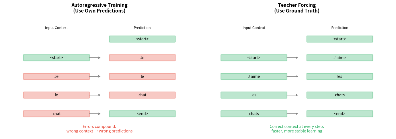
Two approaches emerge from this dilemma. In autoregressive training, the decoder conditions on its own previous predictions. Early in training, these predictions are mostly wrong, meaning the decoder learns from incorrect context. This creates a compounding error problem: one wrong prediction leads to unusual context, which leads to another wrong prediction, and so on.

In teacher forcing, we sidestep this problem entirely by always feeding the decoder the correct previous token from the ground truth sequence. The decoder never sees its own mistakes during training, allowing it to learn from perfect context at every step.

To understand teacher forcing mathematically, we need to think carefully about what information flows into the decoder at each timestep. The decoder's job is to predict the next token, but to do so, it needs context: what tokens came before? This seemingly simple question leads us to two fundamentally different training approaches.

At each timestep $t$, the decoder must produce a prediction for the next token. But the decoder doesn't operate in isolation. It receives two crucial pieces of information:

1. The hidden state $h_t$: This encapsulates everything the decoder has learned from the encoder's representation of the source sequence, plus any information accumulated from previous decoding steps.

2. The previous token: This is where the critical choice arises. Should we give the decoder the token it actually predicted at the previous step, or the token it should have predicted?

This choice fundamentally shapes the learning dynamics.

In standard autoregressive generation, the approach used at inference time, the decoder conditions on its own previous output:

where:

• $\hat{y}_t$: the model's prediction at timestep $t$
• $h_t$: the decoder's hidden state at timestep $t$, encoding information from the encoder and all previous decoding steps
• $\hat{y}_{t-1}$: the model's own prediction from the previous timestep

This formulation mirrors what happens during inference: the model generates a token, then uses that token as context to generate the next one. The appeal is clear: train the model the same way you'll use it.

But there's a problem. Early in training, the model's predictions are essentially random. If $\hat{y}_{t-1}$ is wrong (which it usually is), the decoder receives misleading context. This incorrect context produces a poor hidden state $h_t$, which leads to another incorrect prediction $\hat{y}_t$, which becomes incorrect context for the next step, and so on. Errors don't just occur; they compound.

Teacher forcing sidesteps this compounding problem by replacing the model's prediction with the ground truth:

where:

• $y_{t-1}$: the ground truth token from the target sequence at position $t-1$

The change appears minor (we've simply swapped $\hat{y}_{t-1}$ for $y_{t-1}$), but the implications are profound. By providing the correct previous token, the decoder always operates with ideal context. The learning problem transforms from "given whatever (probably wrong) token you just predicted, what should you predict next?" to "given the correct previous token, what should you predict next?"

This is a much easier problem. The decoder learns the true conditional distribution $P(y_t | y_{<t})$ directly, without the noise introduced by its own errors.

With teacher forcing providing clean context, we can now measure how well the decoder learns. At each timestep, we want to know: given the correct context, how close is the model's prediction to the target?

We use cross-entropy loss, which measures the negative log probability the model assigns to the correct token:

where:

• $\mathcal{L}_t$: the loss at timestep $t$
• $P(y_t | h_t, y_{<t})$: the probability the model assigns to the correct token $y_t$, given the hidden state $h_t$ and all previous ground truth tokens $y_{<t} = (y_1, y_2, \ldots, y_{t-1})$

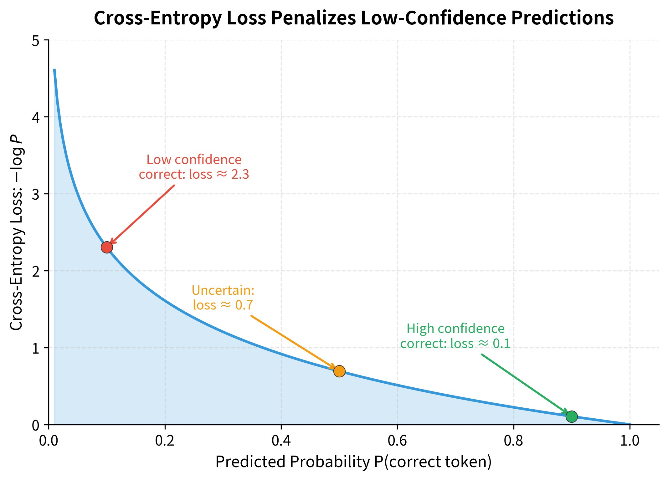
Why negative log probability? Consider what happens as the model improves:

• If the model assigns high probability to the correct token (say, $P = 0.9$), then $-\log(0.9) \approx 0.1$, a small loss.
• If the model assigns low probability (say, $P = 0.1$), then $-\log(0.1) \approx 2.3$, a large loss.

The negative log transforms probabilities into a loss function that penalizes confident wrong predictions heavily while rewarding confident correct predictions.

A sequence contains multiple tokens, each with its own prediction and loss. To train the model, we need a single scalar loss value. The natural choice is to sum the per-timestep losses:

where:

• $\mathcal{L}$: the total loss for the entire sequence
• $T$: the length of the target sequence
• The sum aggregates prediction errors across all positions, treating each timestep's contribution equally

This formulation has an elegant interpretation: we're computing the negative log probability of the entire target sequence under the model's distribution. Minimizing this loss is equivalent to maximizing the probability the model assigns to generating the correct sequence, which is exactly what we want.

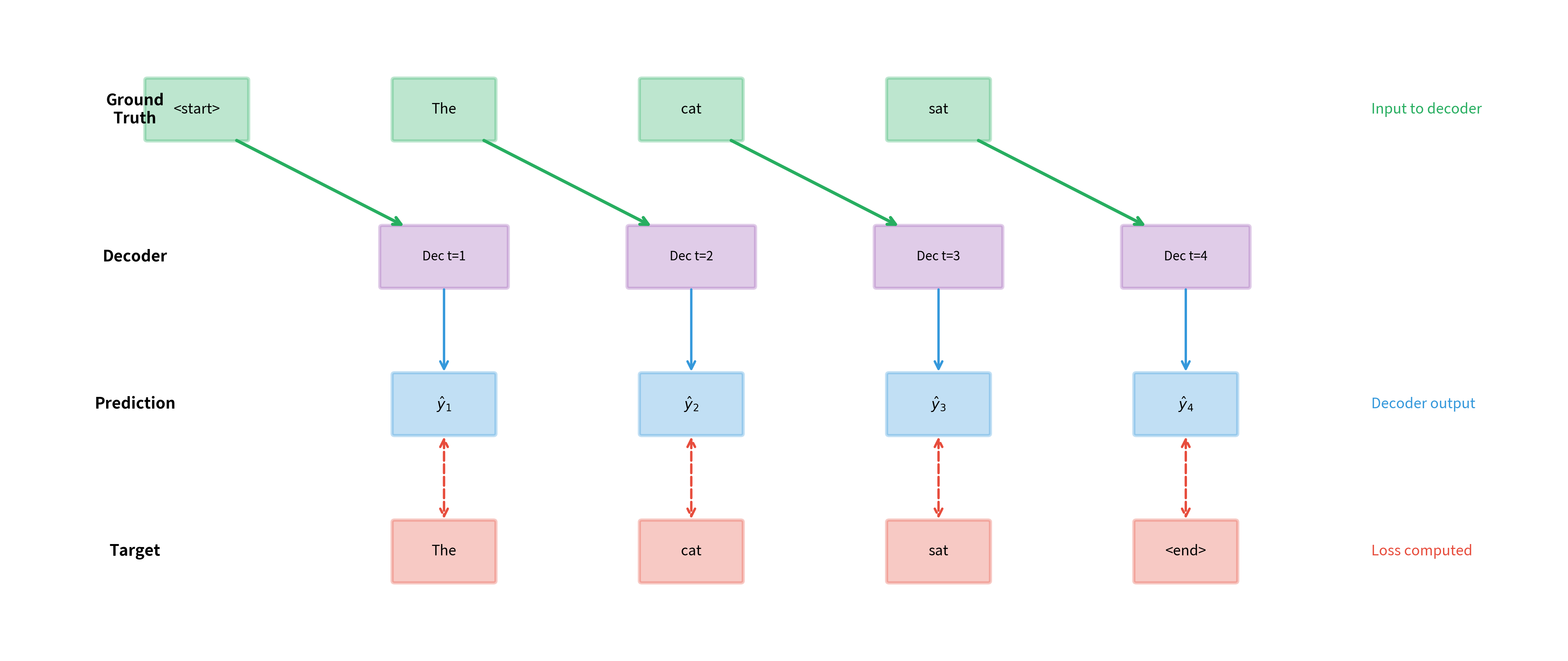
The diagram above illustrates the complete data flow during teacher forcing training. Notice the key insight: the ground truth tokens (green) flow into the decoder as inputs, while the decoder's predictions (blue) flow out for comparison with targets (red). The decoder never sees its own predictions during training. It always receives the correct answer from the previous timestep.

This architecture has a profound consequence: teacher forcing decouples each timestep's learning problem. The model at timestep $t$ learns independently of whether it got timestep $t-1$ correct, because it always receives the correct $y_{t-1}$ regardless. Instead of trying to learn "given my previous (possibly wrong) prediction, what should I predict next?", the model learns "given the correct previous token, what should I predict next?"

This decoupling is what makes teacher forcing so effective, especially early in training when the model would otherwise be learning from a cascade of errors.

Teacher forcing accelerates training for several interconnected reasons. Understanding these helps explain both its effectiveness and, as we'll see later, its limitations.

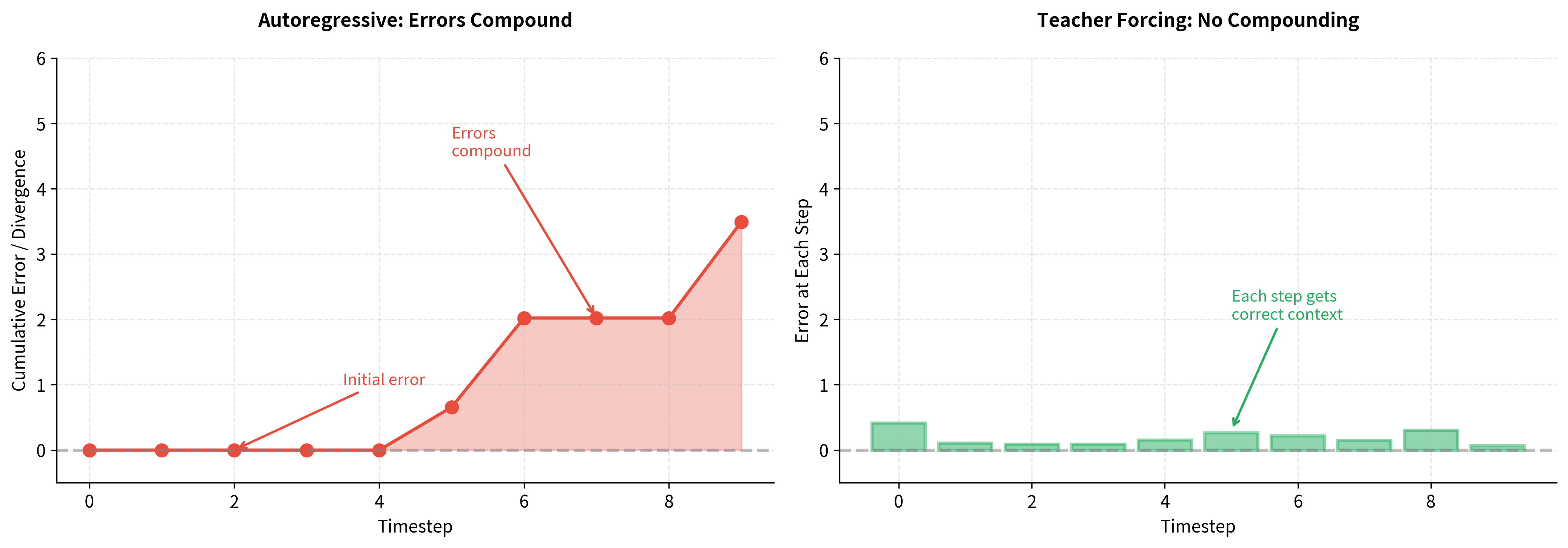
When training with the model's own predictions, errors compound across timesteps. An early mistake creates unusual context, leading to another mistake, which creates even more unusual context. By the end of a long sequence, the decoder might be operating in a completely unfamiliar regime. Gradients computed from such sequences are noisy and can point in unhelpful directions.

Teacher forcing eliminates this compounding. Every timestep receives correct context, so the gradients at each position reflect the true learning signal: "given this correct context, how should I adjust my weights to predict the next token better?" These cleaner gradients lead to faster, more stable convergence.

A less obvious but practically important benefit is computational efficiency. With teacher forcing, we know all the inputs to the decoder before training begins: they're just the ground truth sequence shifted by one position. This means we can compute all timesteps in parallel using matrix operations, rather than sequentially waiting for each prediction.

In frameworks like PyTorch, this translates to feeding the entire target sequence (minus the last token) as input and computing all predictions simultaneously. The speedup is substantial, especially for long sequences where sequential processing would be prohibitively slow.

Let's see this parallel computation in action by processing a batch of sequences:

The decoder processed all 32 sequences of 50 tokens each in a single forward pass, producing predictions over the entire 1000-word vocabulary for every position. This demonstrates the key efficiency gain of teacher forcing: because we know all inputs ahead of time (the ground truth tokens), we can leverage matrix operations to compute everything in parallel rather than waiting for each prediction sequentially.

The parallel computation advantage is significant. Processing 50 timesteps sequentially would require 50 separate forward passes through the RNN, each waiting for the previous one to complete. With teacher forcing, we compute everything in one pass, leveraging GPU parallelism for massive speedups.

Teacher forcing also improves credit assignment during backpropagation. When the model makes a wrong prediction, we want the gradients to teach it "you should have predicted X instead of Y given this context." With autoregressive training, the context itself might be wrong, confusing the learning signal. With teacher forcing, the context is always correct, so the model learns exactly what it should predict in each situation.

This cleaner credit assignment is particularly important for learning rare patterns. If a specific context only appears a few times in the training data, the model needs to learn from each occurrence efficiently. Teacher forcing ensures these learning opportunities aren't wasted on noisy gradients from compounded errors.

Teacher forcing's greatest strength is also its greatest weakness. By always providing correct context during training, we create a mismatch between training and inference conditions. During inference, the model must use its own predictions as context, but it has never practiced doing so. This mismatch is called exposure bias.

The consequences of exposure bias can be severe. A model might perform well on standard metrics like perplexity (which measure prediction quality given correct context) but generate poor outputs when running autoregressively. Small prediction errors that the model never learned to handle can cascade into completely incoherent outputs.

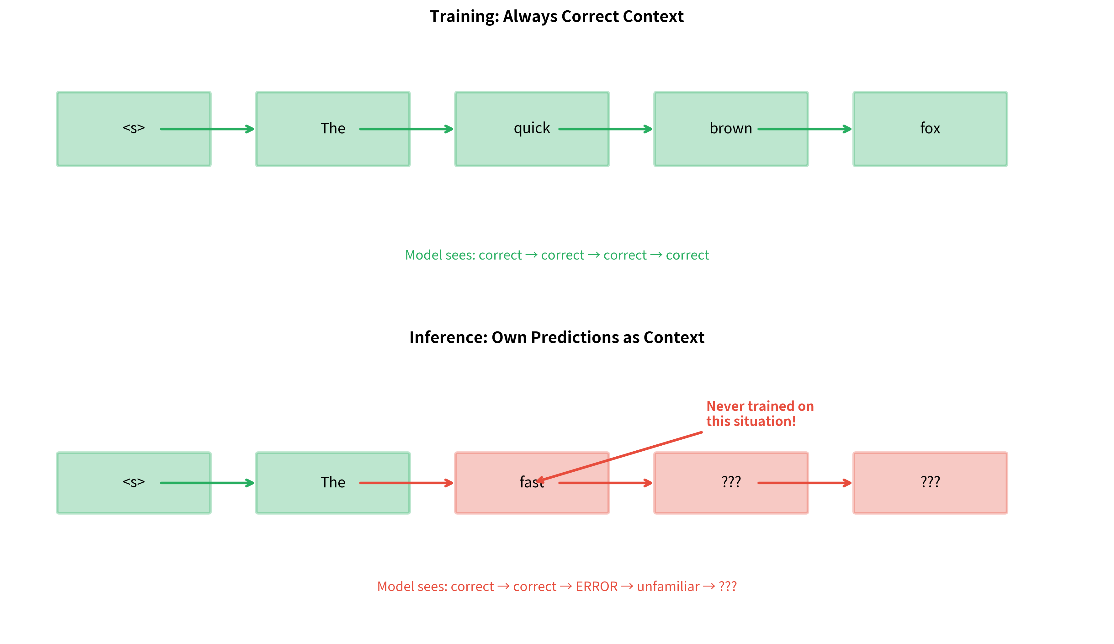
Consider a concrete example. Suppose during inference the model predicts "fast" instead of "quick" in "The quick brown fox." With teacher forcing, the model has never seen the context "The fast" followed by anything, so it has no idea what to predict next. It might output something reasonable by chance, or it might produce nonsense. The model simply wasn't trained to handle this situation.

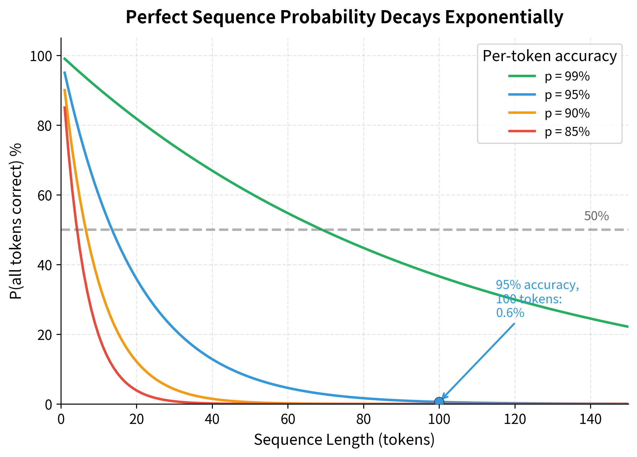
The exposure bias problem becomes more severe as sequences get longer. Each timestep has some probability of error, and these probabilities compound. Consider a sequence of length $T$ where each token has probability $p$ of being predicted correctly. If we assume each prediction is independent (a simplification, but useful for intuition), the probability of generating the entire sequence without any errors is simply the product of getting each individual token correct:

where:

• $P(\text{all\_correct})$: the probability of generating the complete sequence without any errors
• $p$: the probability of correctly predicting a single token (e.g., 0.95 for 95% accuracy)
• $T$: the total sequence length (number of tokens to generate)
• $p^T$: the probability that all $T$ independent predictions are correct, computed by multiplying $p$ by itself $T$ times

This formula reveals why exposure bias becomes increasingly problematic for longer sequences. For a 100-token sequence with 95% per-token accuracy, the probability of a completely correct sequence is only $(0.95)^{100} \approx 0.006 = 0.6\%$. The model will almost certainly encounter its own mistakes, yet it has no experience dealing with them.

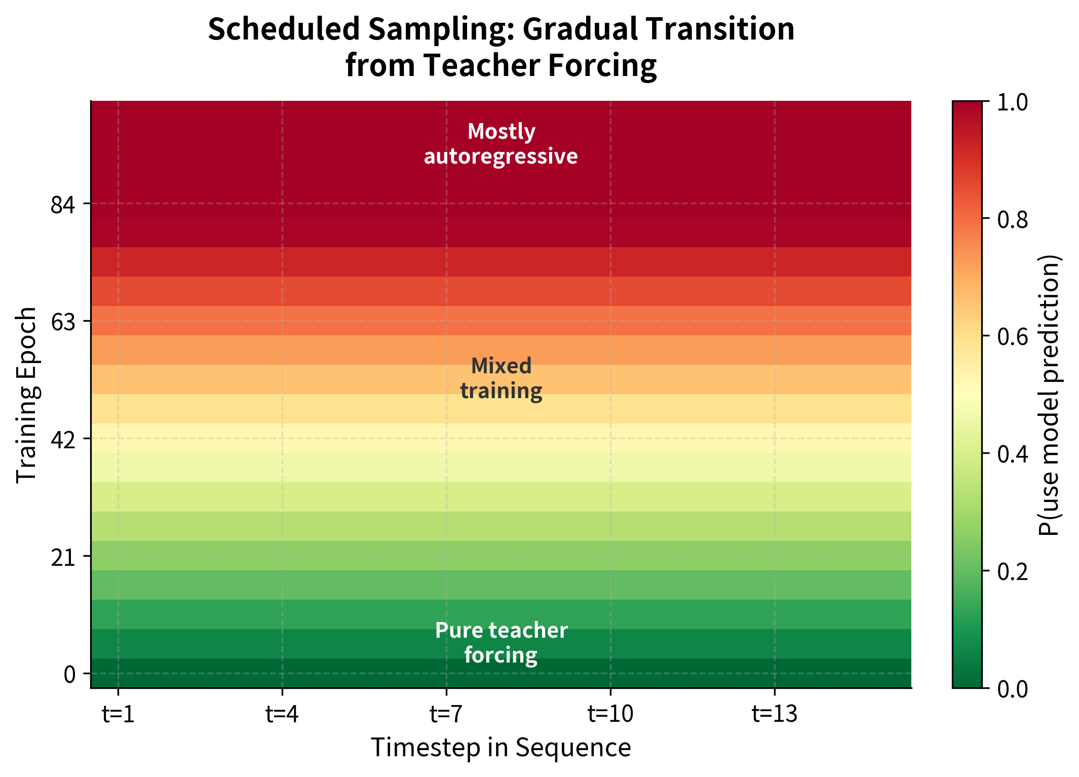
Scheduled sampling, introduced by Bengio et al. (2015), offers a compromise between pure teacher forcing and pure autoregressive training. The idea is simple: during training, randomly decide at each timestep whether to use the ground truth token or the model's own prediction as input to the next step. Early in training, use ground truth most of the time (like teacher forcing). As training progresses, gradually increase the probability of using the model's own predictions.

The schedule can take various forms, each defined by a function that maps the current epoch to a sampling probability $\epsilon$:

Linear schedule: The probability increases at a constant rate until reaching 1.0:

where:

• $\epsilon(e)$: the sampling probability at epoch $e$ (probability of using the model's own prediction rather than ground truth)
• $e$: the current training epoch (starting from 0)
• $E_{\max}$: the epoch at which to reach full autoregressive training (typically set to 80% of total epochs)
• $\min(1, \cdot)$: ensures the probability never exceeds 1.0

The linear schedule increases the sampling probability by $\frac{1}{E_{\max}}$ each epoch. For example, if $E_{\max} = 80$ and total training is 100 epochs, the probability increases by 0.0125 per epoch until reaching 1.0 at epoch 80, then remains at 1.0 for the final 20 epochs.

Exponential schedule: The probability grows quickly at first, then slows as it approaches 1.0:

where:

• $\epsilon(e)$: the sampling probability at epoch $e$
• $k$: a decay constant slightly less than 1 (e.g., 0.97), controlling how quickly teacher forcing is phased out
• $e$: the current training epoch
• $k^e$: the teacher forcing probability, which decays exponentially toward 0

The intuition is that $k^e$ represents the probability of still using teacher forcing. Since $k < 1$, this value shrinks exponentially: at epoch 0, $k^0 = 1$ (100% teacher forcing); as $e$ increases, $k^e \to 0$. Subtracting from 1 gives us the probability of using the model's own predictions instead.

Inverse sigmoid schedule: Provides a smooth S-curve transition:

where:

• $\epsilon(e)$: the sampling probability at epoch $e$
• $c$: the midpoint epoch where $\epsilon = 0.5$ (the center of the S-curve)
• $b$: controls the steepness of the transition (larger $b$ means gentler slope, smaller $b$ means sharper transition)
• $e$: the current training epoch
• $\exp(\cdot)$: the exponential function

This is the standard logistic sigmoid function, shifted and scaled. When $e = c$, the exponent becomes 0, so $\exp(0) = 1$ and $\epsilon(c) = \frac{1}{1+1} = 0.5$. When $e \ll c$ (early training), the exponent is large and positive, making $\epsilon(e) \approx 0$. When $e \gg c$ (late training), the exponent is large and negative, making $\epsilon(e) \approx 1$.

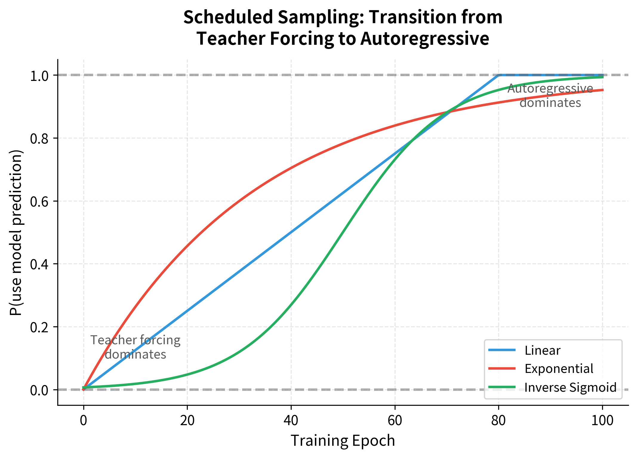
The choice of schedule is a hyperparameter that may need tuning for different tasks. Linear schedules are simple and predictable, exponential schedules transition faster early on, and inverse sigmoid schedules provide the smoothest transition with gradual changes at both ends.

Let's implement scheduled sampling and see how it affects training:

At epoch 0, all schedules start with probability 0.000 (pure teacher forcing), meaning the model always receives ground truth context. By epoch 50, the schedules diverge significantly: exponential reaches 0.782, linear is at 0.625, and inverse sigmoid sits exactly at its designed midpoint of 0.500. The exponential schedule transitions fastest early on, making it suitable when you want to reduce teacher forcing quickly. The inverse sigmoid provides the smoothest transition overall, with gradual changes at both the beginning and end of training.

The choice of schedule affects how the model experiences the transition from ideal training conditions to realistic inference conditions. Linear schedules are predictable and easy to reason about, exponential schedules front-load the transition, and inverse sigmoid schedules minimize abrupt changes.

Scheduled sampling has both benefits and drawbacks:

• Benefits: Reduces exposure bias by gradually exposing the model to its own predictions. The model learns to handle imperfect context before it must do so at inference time.
• Drawbacks: Training becomes sequential (no parallel computation), significantly slower than pure teacher forcing. The schedule introduces additional hyperparameters. The method doesn't eliminate exposure bias entirely, just reduces it.

Curriculum learning takes a different approach to the training-inference mismatch. Instead of changing what context the model sees, we change what sequences the model learns on. The idea is to start with "easy" examples and gradually introduce harder ones, mimicking how humans learn.

For sequence generation, "easy" might mean:

• Shorter sequences: Easier because there are fewer opportunities for errors to compound
• More common patterns: Easier because the model has seen them more often
• Lower perplexity targets: Easier because the next token is more predictable

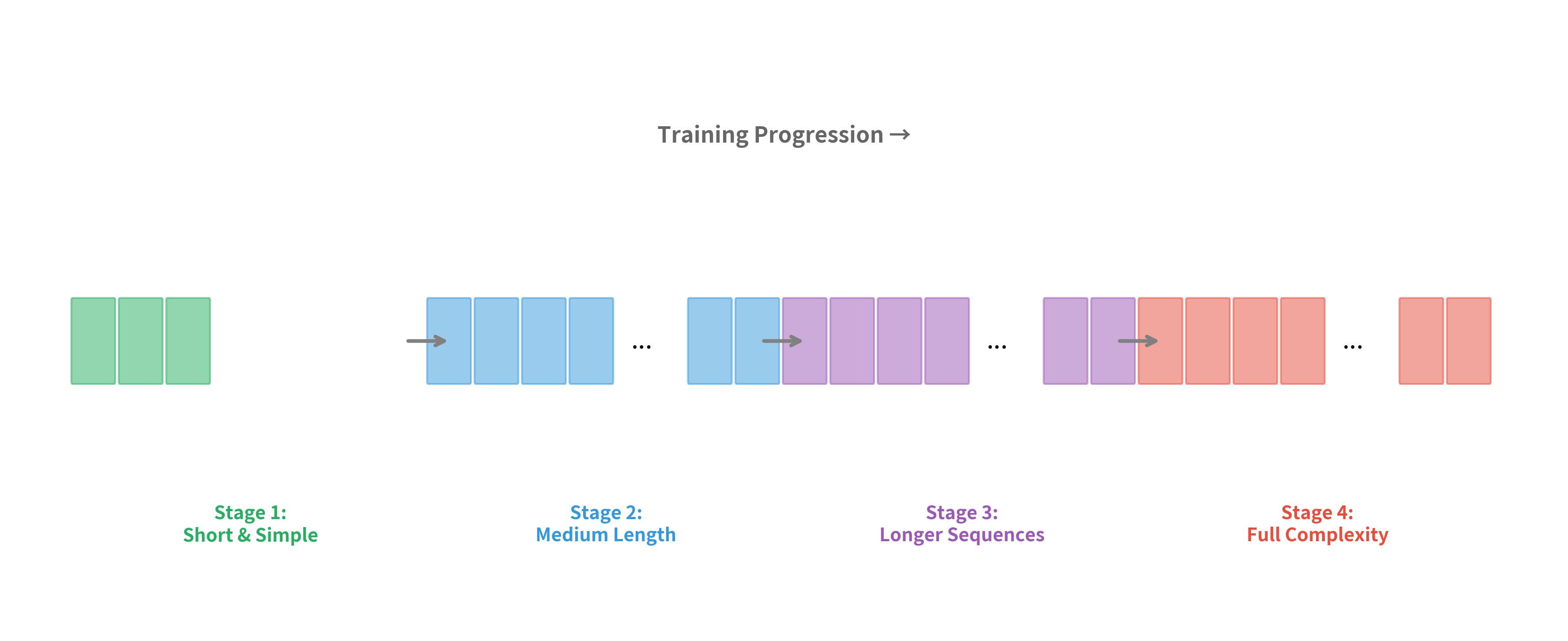
Implementing curriculum learning for sequence generation typically involves sorting training examples by difficulty and presenting them in order:

The curriculum organizes examples by increasing difficulty. Stage 1 contains only the shortest translations (3-character targets like "Oui"), allowing the model to learn basic encoder-decoder mechanics before tackling complexity. Each subsequent stage includes all previous examples plus longer ones, ensuring the model doesn't forget simpler patterns while learning harder ones. By Stage 3, the model trains on the full dataset including long translations like "Comment allez-vous aujourd'hui mon ami".

Curriculum learning helps with exposure bias indirectly. By mastering short sequences first, the model builds robust representations before encountering the long sequences where exposure bias is most problematic. However, it doesn't directly address the training-inference mismatch.

Let's compare the different training approaches empirically. We'll train simple sequence-to-sequence models using teacher forcing, scheduled sampling, and a baseline autoregressive approach, then evaluate their behavior.

Teacher forcing achieves faster convergence, reaching low loss values earlier in training. The scheduled sampling model shows more variance in its loss curve because it increasingly uses its own (sometimes incorrect) predictions as training progresses.

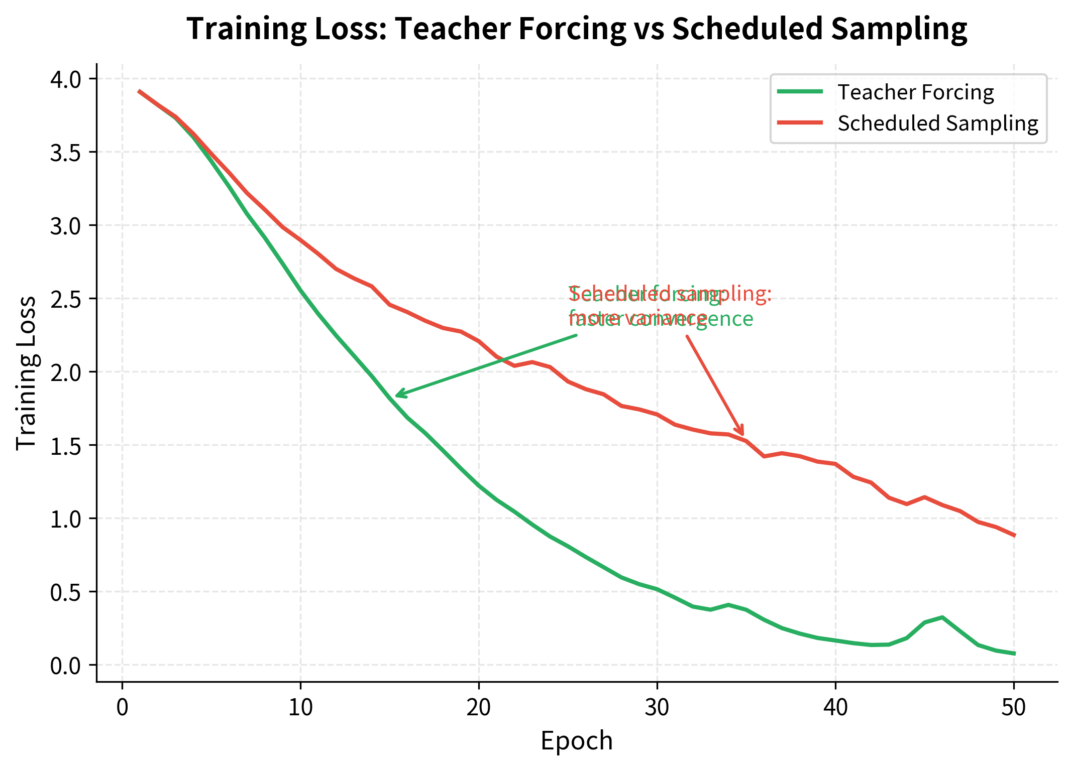
The training curves reveal the trade-offs between these approaches. Teacher forcing shows rapid, stable convergence because every timestep receives correct context and gradients flow cleanly. Scheduled sampling shows more variance, especially in later epochs when the model increasingly sees its own predictions. However, the scheduled sampling model may generalize better to the autoregressive inference setting.

Let's evaluate both models on autoregressive generation to see if scheduled sampling's additional training cost pays off:

Both models achieve high accuracy on this simple copy task, which requires the decoder to reproduce the input sequence exactly. The copy task is relatively easy because there's a direct one-to-one mapping between input and output tokens. For this task, the exposure bias from teacher forcing doesn't cause significant problems because the learned mapping is robust.

The results depend on the specific task and model capacity. For simple tasks like copying, teacher forcing often performs well because the model learns a robust mapping. For more complex tasks with longer sequences, scheduled sampling's exposure to its own predictions during training can provide meaningful benefits.

Based on the trade-offs we've explored, here are practical guidelines for choosing and implementing training strategies:

Start with teacher forcing. It's simple, fast, and often sufficient. The parallel computation advantage alone makes it the default choice for initial experiments. Many successful production systems use pure teacher forcing without significant issues.

Consider scheduled sampling when:

• Your sequences are long (50+ tokens)
• You observe a large gap between training perplexity and generation quality
• You have the computational budget for slower training
• Your task involves open-ended generation where small errors can cascade

Implement curriculum learning when:

• You have a natural difficulty ordering for your data
• Training is unstable or slow to converge
• You're working with limited data and need efficient learning

Monitor for exposure bias by:

• Comparing teacher-forced perplexity with autoregressive generation quality
• Examining generated outputs for characteristic "drift" where early errors compound
• Testing on sequences longer than those seen during training

Teacher forcing revolutionized sequence-to-sequence training by making it practical to train deep models on long sequences. Before teacher forcing, training decoders was slow and unstable, with errors compounding unpredictably. The technique enabled the first successful neural machine translation systems and remains the default training approach for most sequence generation models.

However, exposure bias remains a fundamental limitation. The mismatch between training and inference conditions means that models may behave unpredictably when they encounter their own errors. This is particularly problematic for open-ended generation tasks like story writing or dialogue, where there's no single correct output and the model must maintain coherence over many tokens.

The research community continues to develop alternatives. Reinforcement learning approaches like REINFORCE and actor-critic methods can train directly on generation quality metrics, avoiding the exposure bias problem entirely. However, these methods are harder to train and often less stable than teacher forcing. Minimum risk training optimizes expected loss under the model's own distribution, providing another path forward.

More recently, large language models trained with teacher forcing have shown remarkable generation quality despite the theoretical exposure bias concern. This suggests that with sufficient model capacity and data, the practical impact of exposure bias may be smaller than theory predicts. Nevertheless, understanding the trade-offs remains important for practitioners working with smaller models or specialized domains.

Teacher forcing is a training technique that provides the decoder with ground truth context at each timestep rather than its own predictions. This simple change has profound effects on training dynamics.

The key benefits of teacher forcing are:

• Faster convergence: Clean gradients from correct context enable rapid learning
• Parallel computation: Knowing all inputs in advance allows efficient batch processing
• Stable training: No error compounding means consistent learning signal

The main drawback is exposure bias: the model trains on a different distribution than it encounters during inference. This can cause generation quality to degrade, especially for long sequences.

Mitigation strategies include:

• Scheduled sampling: Gradually transition from teacher forcing to autoregressive training
• Curriculum learning: Start with easy examples and progressively increase difficulty
• Reinforcement learning: Train directly on generation metrics (covered in later chapters)

For most practical applications, start with pure teacher forcing. It's simple, fast, and often sufficient. Consider alternatives when you observe a significant gap between training metrics and generation quality, or when working with very long sequences where exposure bias is most pronounced.

The next chapter explores beam search, a decoding strategy that addresses a different aspect of sequence generation: how to find high-quality outputs from the model's learned distribution during inference.

When implementing teacher forcing and its alternatives, several parameters significantly impact training behavior and model performance:

• teacher_forcing_ratio (for scheduled sampling): The probability of using ground truth versus model predictions at each timestep. A value of 1.0 means pure teacher forcing, while 0.0 means pure autoregressive training. Start with 1.0 and decrease over training epochs.

• schedule_type: Controls how the teacher forcing ratio changes over time. Options include "linear" (steady decrease), "exponential" (fast initial decrease), and "inverse_sigmoid" (smooth S-curve). Linear is simplest to tune, while inverse sigmoid provides the smoothest transition.

• warmup_epochs: Number of epochs to use pure teacher forcing before starting the scheduled transition. Allows the model to learn basic patterns before introducing its own predictions. Typical values range from 5-20% of total training epochs.

• k (exponential schedule): Decay constant controlling how quickly teacher forcing decreases. Values close to 1.0 (e.g., 0.97-0.99) provide gradual transitions, while smaller values accelerate the shift to autoregressive training.

• c and b (inverse sigmoid schedule): The midpoint epoch ($c$) and steepness ($b$) of the sigmoid transition. Setting $c$ to half the total epochs and $b$ to 10% of total epochs provides a balanced S-curve.

• curriculum_stages: Number of difficulty stages when using curriculum learning. More stages (4-6) provide finer-grained progression but require more careful difficulty scoring. Fewer stages (2-3) are simpler but may have abrupt difficulty jumps.

Ready to test your understanding? Take this quick quiz to reinforce what you've learned about teacher forcing and training strategies for sequence-to-sequence models.