

Learn how dropout prevents overfitting by randomly dropping neurons during training, creating an implicit ensemble of sub-networks for better generalization.

This article is part of the free-to-read Language AI Handbook
Choose your expertise level to adjust how many terms are explained. Beginners see more tooltips, experts see fewer to maintain reading flow. Hover over underlined terms for instant definitions.
Dropout
Neural networks are remarkably powerful function approximators. With enough parameters, they can memorize training data perfectly, achieving near-zero training loss. But this very power creates a fundamental problem: overfitting. A model that memorizes training examples fails to generalize to new, unseen data.
Dropout offers a simple but effective solution. During training, we randomly "drop" neurons by setting their outputs to zero. This seemingly destructive intervention forces the network to develop redundant representations, preventing any single neuron from becoming too specialized. The result is a more robust model that generalizes better to new data.
This chapter explores dropout from multiple perspectives. We'll see how dropout implicitly trains an ensemble of networks, understand the mathematics of inverted dropout scaling, implement dropout from scratch, and examine how modern architectures adapt dropout to their specific needs.
The Overfitting Problem
Before diving into dropout, let's understand why neural networks overfit and why traditional regularization alone isn't enough.
A neural network with millions of parameters can represent incredibly complex functions. Given enough capacity, it will find ways to perfectly fit the training data, including noise and outliers. The problem isn't finding a good fit; it's finding a fit that transfers to new data.
Consider a simple experiment: a network trained to classify sentiment. With enough hidden units, it might learn that "review #1247 is positive" rather than learning generalizable patterns like "words like 'excellent' and 'amazing' indicate positive sentiment."
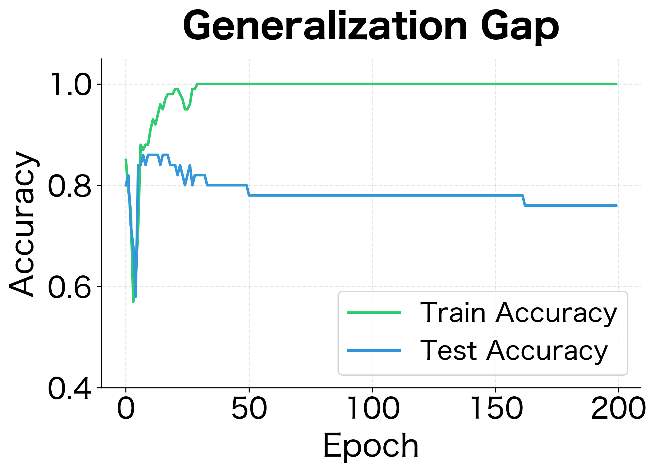
The gap between training and test accuracy is the hallmark of overfitting. The network has learned patterns specific to the training data that don't generalize. Traditional L2 regularization helps but doesn't fully solve the problem, especially for deep networks with complex interdependencies between neurons.
Dropout as Implicit Ensemble
Dropout was introduced by Hinton et al. (2012) with a key insight: randomly dropping neurons during training is equivalent to training an exponentially large ensemble of sub-networks.
Dropout is a regularization technique where, during training, each neuron's output is set to zero with probability (the dropout rate). The remaining neurons are kept with probability . At test time, all neurons are active, but their outputs are scaled appropriately.
Consider a network with neurons in a layer. During a single training step with dropout, we randomly select a subset of these neurons to keep active. This effectively creates a "thinned" network, a sub-network using only the active neurons.
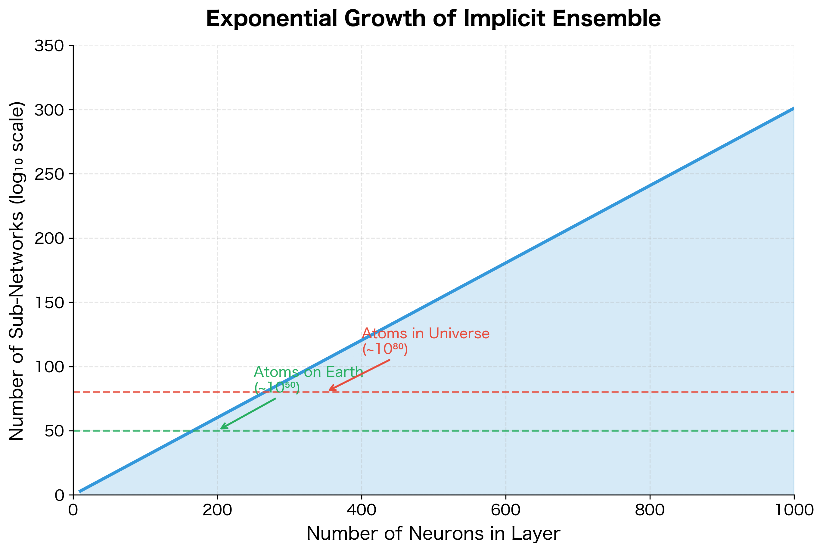
How many possible sub-networks exist? For each neuron, we have two choices: keep it or drop it. With neurons, this gives possible sub-networks. A layer with just 1000 neurons produces more sub-networks than atoms in the observable universe.
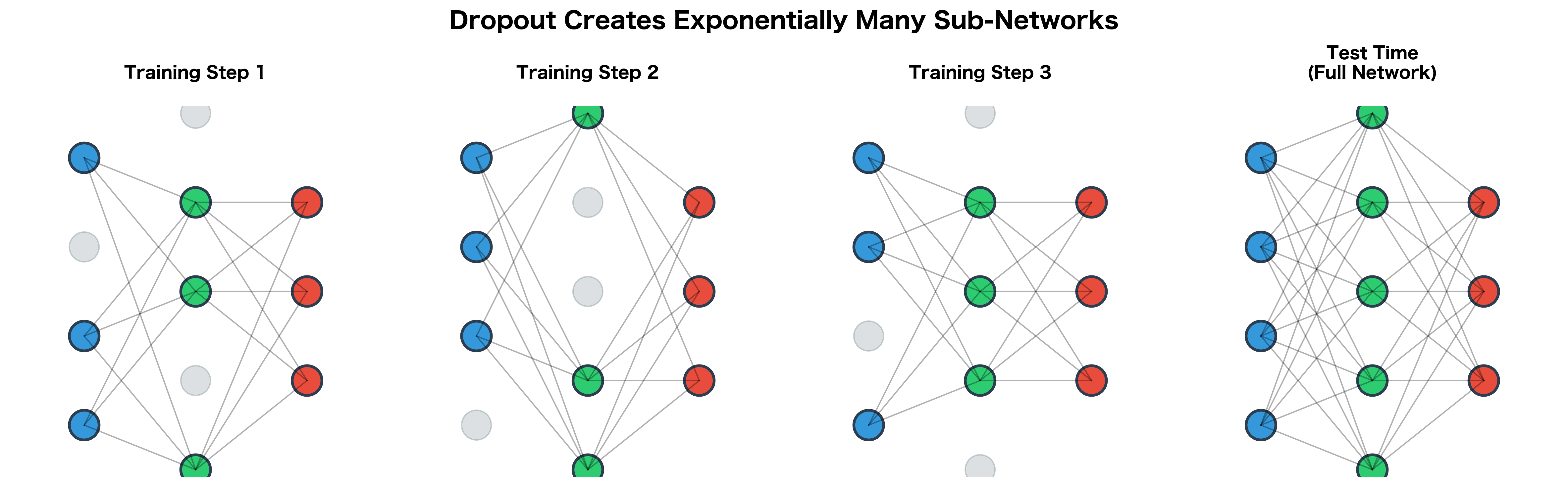
Each training batch sees a different sub-network. Over many training steps, we effectively train all possible sub-networks, though each one receives only a small amount of training. The remarkable result is that this ensemble training occurs implicitly through weight sharing: all sub-networks share the same underlying parameters.
At test time, instead of averaging predictions from sub-networks (computationally impossible), we use all neurons but scale their outputs. This scaling approximates the ensemble average, giving us the benefit of ensemble methods without the computational cost.
The Dropout Mechanism
Now that we understand the intuition behind dropout, let's formalize the mathematics. The key question is: how do we randomly "turn off" neurons in a way that's both computationally efficient and mathematically sound?
The Masking Operation
Consider a layer in our network that has just computed its activations. Before passing these activations to the next layer, we want to randomly zero out some of them. The natural way to do this is through a binary mask: a vector of ones and zeros that we multiply element-wise with the activations.
For a layer with activation vector of dimension , dropout applies:
where:
- : the original activation vector (what the layer computed before dropout)
- : a binary mask vector of the same dimension, where each element is either 0 (drop) or 1 (keep)
- : element-wise multiplication (Hadamard product)
- : the masked activation vector that continues through the network
The mask is randomly generated fresh for each training example. Each element is independently sampled from a Bernoulli distribution with parameter :
This means each neuron has probability of being dropped (set to zero) and probability of being kept. The independence is crucial: we make a separate random decision for each neuron, creating a different sparse pattern for every training example.
Let's see this in action with a concrete example. We'll apply dropout with to a vector of 8 activations:
The mask randomly selected neurons 2, 5, and 7 to keep (mask = 1) while dropping the others (mask = 0). When we multiply element-wise, the dropped neurons become exactly zero, while the kept neurons retain their original values.
The Scale Mismatch Problem
This naive implementation has a subtle but critical flaw. Consider what happens to the expected total activation:
- During training: With , roughly half the neurons are zeroed, so the expected sum of activations is cut in half.
- During inference: We use all neurons (no dropout), so the full sum of activations flows through.
This mismatch means the network sees different activation magnitudes during training versus testing. Downstream layers receive signals of different scales depending on whether we're training or not. This can cause the model to behave erratically at test time.
Inverted Dropout: The Standard Implementation
There are two ways to fix the scale mismatch:
- Standard dropout: Keep training unchanged, but scale activations by at test time to reduce them
- Inverted dropout: Scale activations by during training, use the network unchanged at test time
Modern implementations universally use inverted dropout. Why? Because it moves all the complexity to training time, leaving inference clean and simple. At deployment, you just run the network normally with no special handling.
Inverted dropout scales activations during training by rather than scaling at test time. This ensures the expected value of each activation remains unchanged, and test time requires no modification.
Deriving the Scaling Factor
Let's work through the math to understand why is exactly the right scaling factor.
With inverted dropout, the output for each neuron becomes:
where:
- : the output activation after dropout is applied
- : the binary mask value for neuron (either 0 or 1)
- : the dropout rate (probability of dropping a neuron)
- : the original activation value for neuron
- : the inverted dropout scaling factor
We want the expected output to equal the original activation. Let's verify this by computing the expectation:
Since is a Bernoulli random variable with parameter , its expected value is simply the probability of being 1:
Substituting back:
The expected output equals the original activation. This means that, on average across many training examples, the network sees the same activation magnitudes it will see at test time.
The intuition is straightforward: if you're keeping a fraction of your neurons, you need to amplify the kept ones by to compensate. With , you keep half and double them. With , you keep 80% and scale by 1.25.
Implementation
With this understanding, we can implement inverted dropout properly:
The backward pass applies the same mask and scaling. Dropped neurons receive zero gradient because they didn't contribute to the forward pass. Kept neurons receive gradients scaled by the same factor, maintaining consistency.
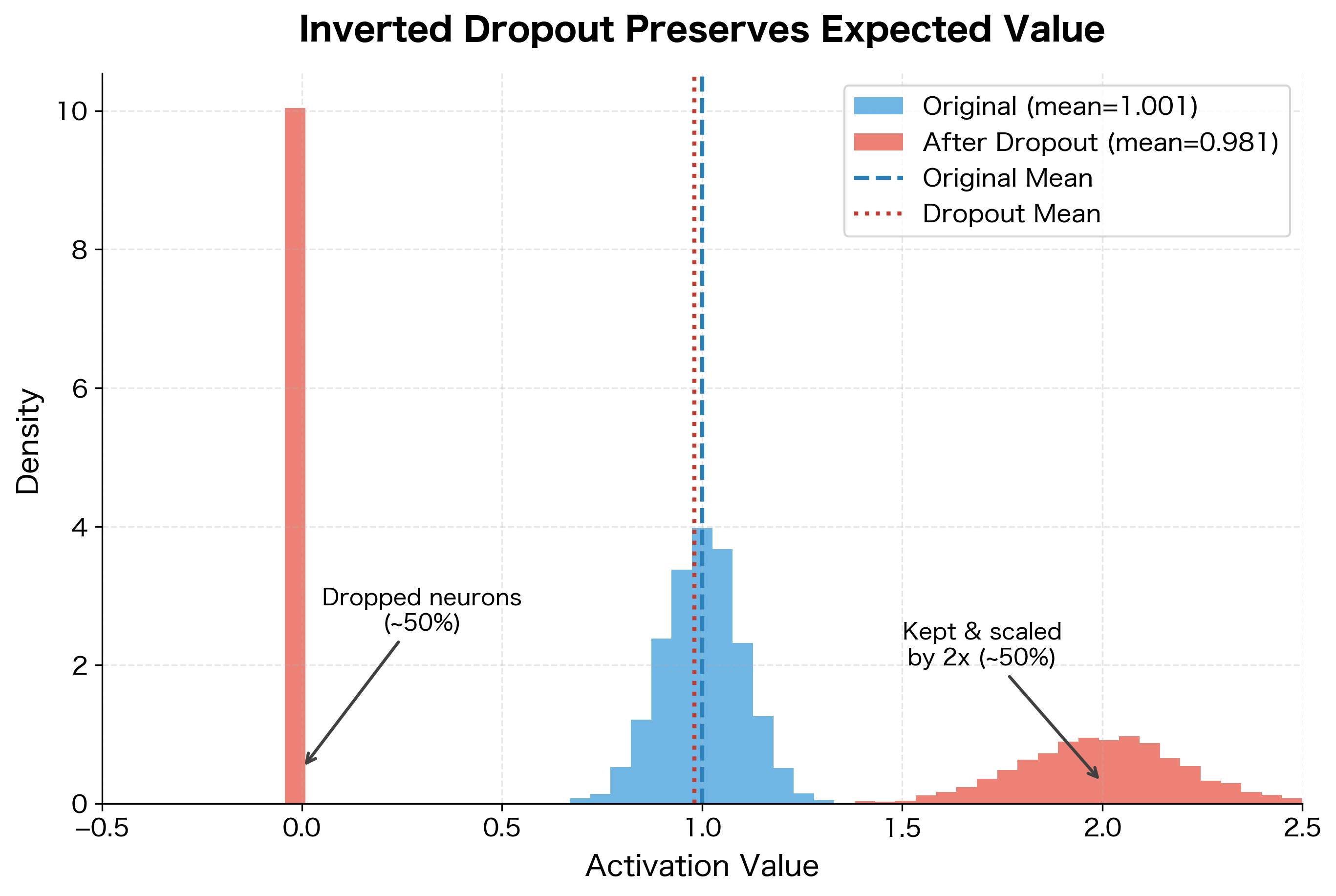
Let's verify empirically that the expected activation is preserved:
With 1000 samples, the empirical mean closely matches the original activation of 1.0, even though half the values are zeros and the other half are doubled. The law of large numbers ensures this averaging works reliably in practice.
Visualizing Dropout's Effect
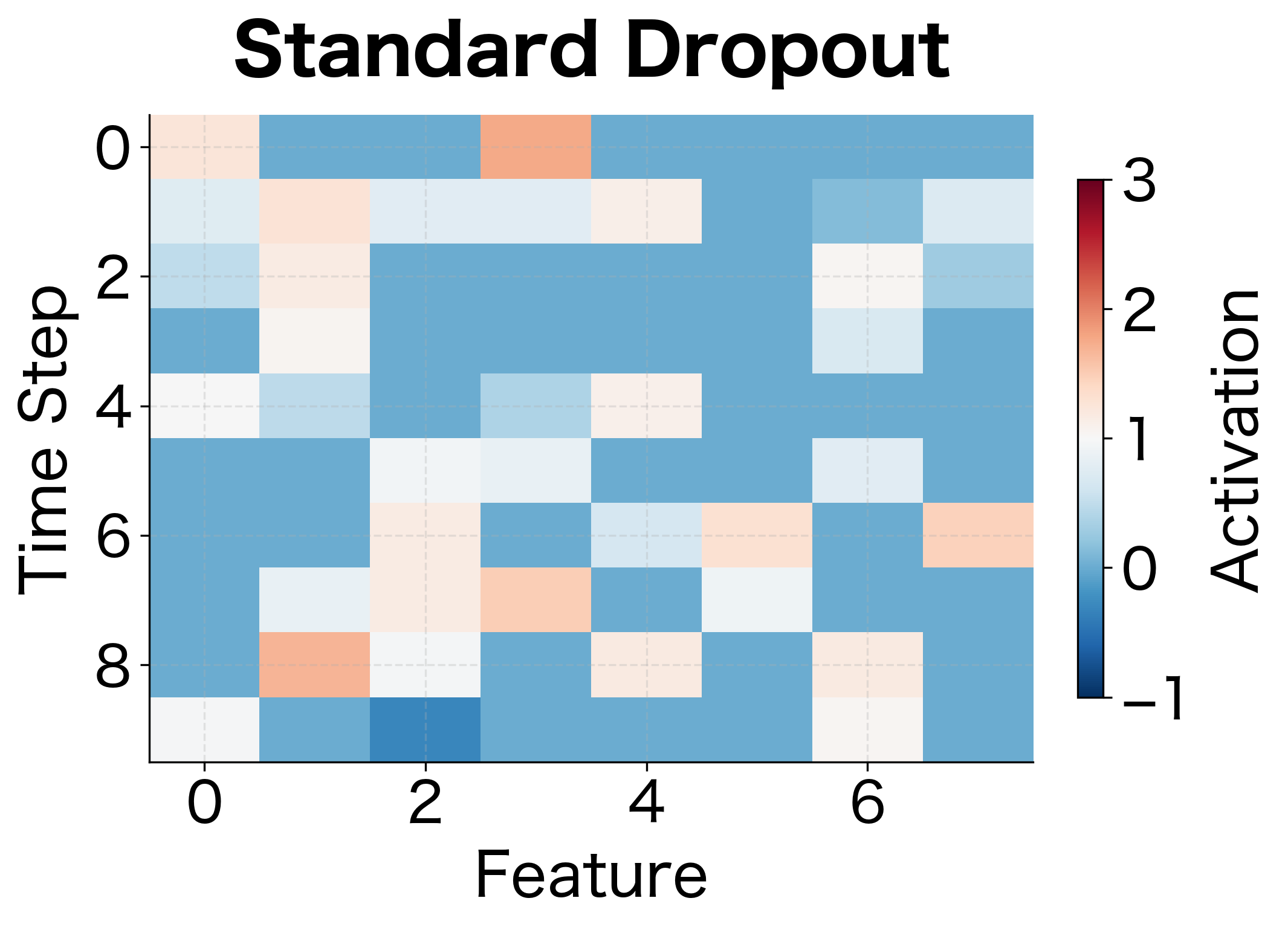
Let's visualize how dropout affects the activation patterns across a layer. We'll see that dropout creates sparse, varying activation patterns that force the network to develop redundant representations.
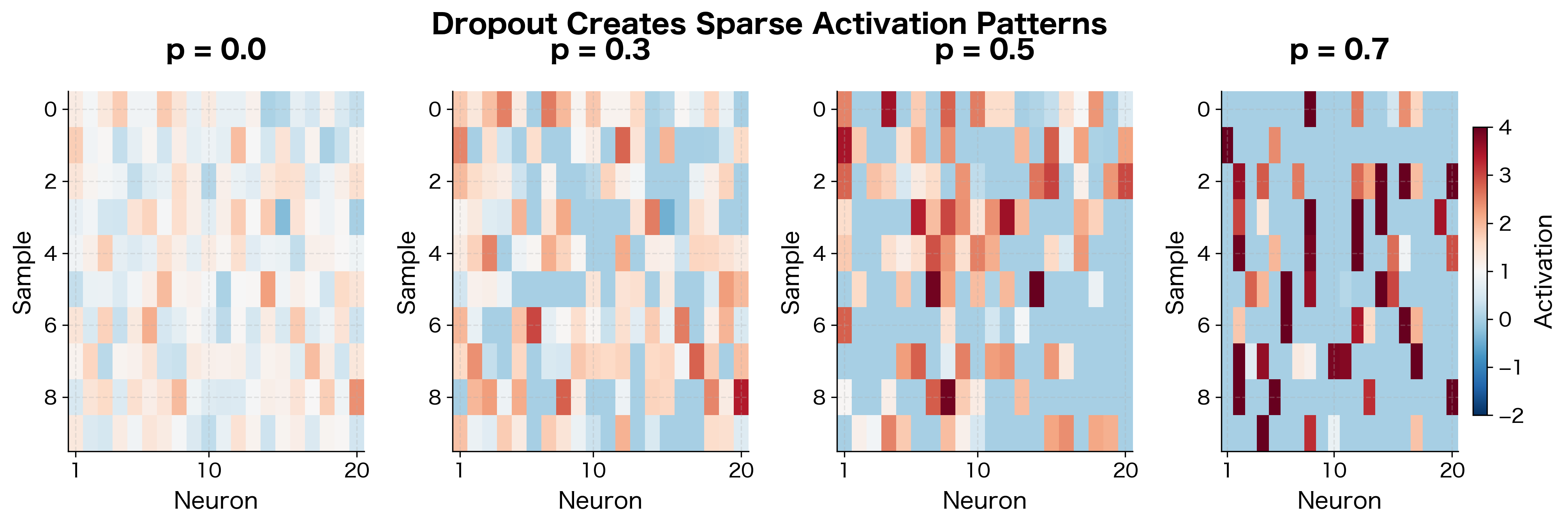
The white regions show dropped neurons. With higher dropout rates, the network must rely on fewer neurons for each prediction, encouraging it to spread important information across many neurons rather than depending on a few specialized ones.
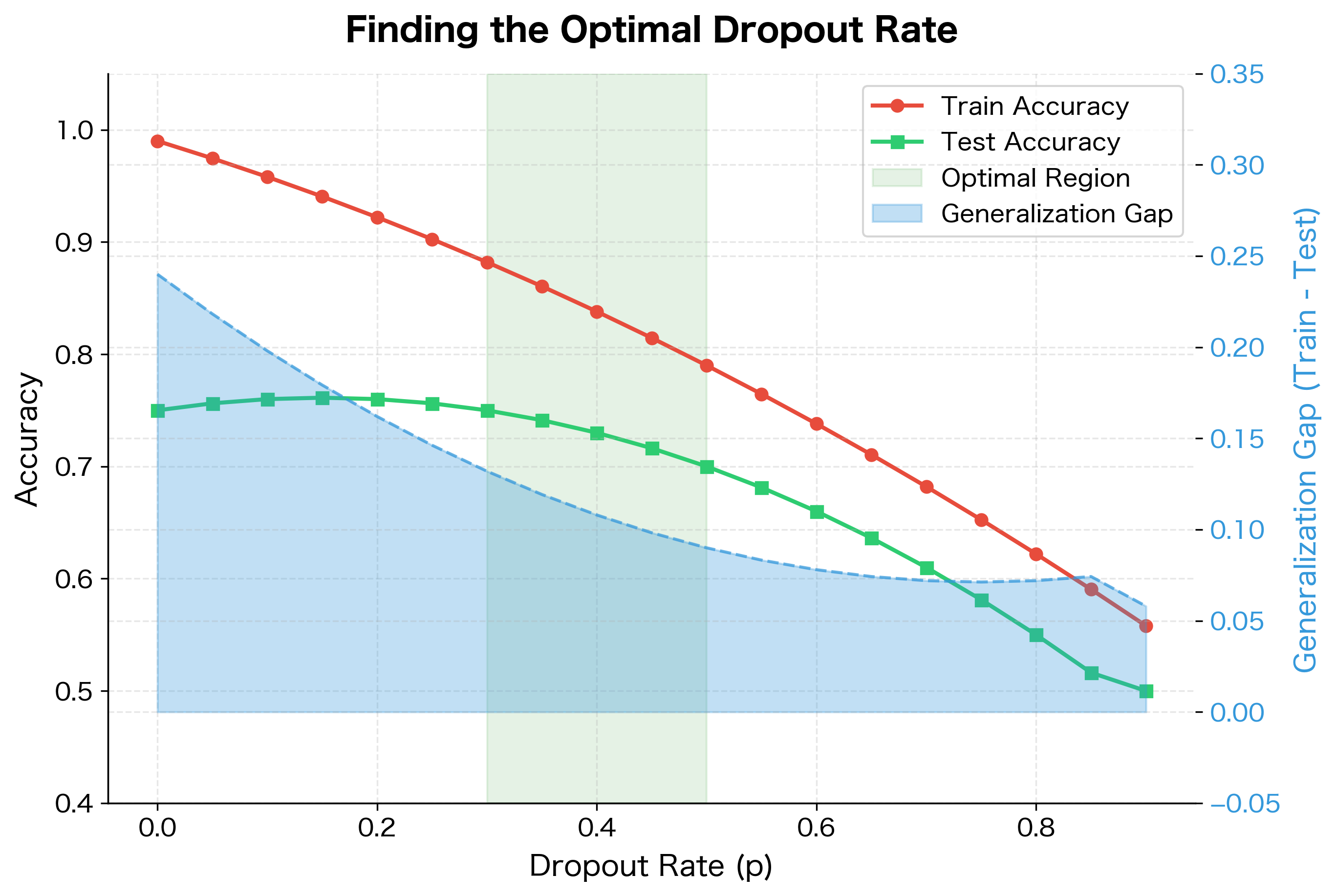
Choosing the Dropout Rate
The dropout rate is a hyperparameter that balances regularization strength against information flow. Too little dropout provides insufficient regularization; too much destroys the signal entirely.
Common guidelines for dropout rates include:
- Input layer: to . Dropping too many input features discards potentially useful information.
- Hidden layers: is the classic default, recommended in the original paper. It maximizes the number of possible sub-networks.
- Output layer: Usually no dropout. The output layer needs to produce consistent predictions.
The optimal rate depends on several factors. Larger networks can handle higher dropout rates since they have more redundancy. Smaller datasets benefit from stronger regularization (higher ). Complex tasks may require lower dropout to preserve learning capacity.
The original Dropout paper by Hinton et al. showed that for hidden layers and for input layers worked well across many tasks. However, modern practice often uses lower rates ( to ) in combination with other regularization techniques like batch normalization.
Dropout at Inference Time
A common source of bugs is forgetting to disable dropout at inference time. During inference (testing, prediction, deployment), we want deterministic, reproducible outputs. Using all neurons without dropout gives us the "average" prediction of the ensemble.
The key insight is that inverted dropout makes inference trivially simple: just use the network as-is, with no modifications. All the scaling was handled during training.
This train/eval distinction is critical. Forgetting to call model.eval() before inference is a common bug that causes inconsistent predictions and degraded test performance.
A Worked Example: Dropout in a Simple Network
Abstract formulas become concrete through worked examples. Let's trace through exactly how dropout affects both the forward and backward passes in a complete network, using specific numbers at each step. By following the mathematics with real values, you'll develop an intuition for how dropout operates during training.
Setting Up the Network
Consider a simple two-layer network for binary classification:
- Input: (a 2-dimensional feature vector)
- Hidden layer: 4 neurons with ReLU activation
- Output layer: 1 neuron (for binary classification)
- Dropout: Applied after the hidden layer with
The network has weights (shape ), biases (length 4), weights (shape ), and bias (scalar).
Step 1: Computing Hidden Activations
The input first passes through the hidden layer. We compute a linear transformation followed by ReLU activation:
where:
- : the input vector
- : the weight matrix connecting input to hidden layer
- : the bias vector for the hidden layer
- : returns element-wise, zeroing negative values
- : the resulting hidden activations
Suppose this computation produces . All four neurons have positive activations, so none were zeroed by ReLU.
Step 2: Applying Dropout
Here's where the magic happens. Before these activations continue to the output layer, we apply dropout with .
First, we sample a random binary mask:
This particular mask keeps neurons 1 and 3 while dropping neurons 2 and 4. With inverted dropout, we multiply by the mask and scale by :
Notice what happened: neurons 2 and 4 became exactly zero, while neurons 1 and 3 were doubled. The sum of the original activations was . The sum after dropout is . On any single example, the sums won't match exactly, but on average over many examples, the expected sums are equal.
Step 3: Computing the Output
The masked activations now flow to the output layer:
where:
- : the dropout-masked hidden activations
- : the weight matrix connecting hidden to output layer
- : the output layer bias
- : the network's output (before sigmoid activation)
The key observation: only neurons 1 and 3 contribute to the output. Neurons 2 and 4, having zero activations, contribute nothing regardless of their weights. This is how dropout effectively trains a sub-network that excludes certain neurons.
Step 4: Backpropagation Through Dropout
During training, we compute a loss and backpropagate gradients. When the gradient reaches the dropout layer, we apply the same mask:
where:
- : the loss function being minimized
- : the gradient flowing back from the output layer
- : the same binary mask used in the forward pass
- : the inverted dropout scale factor
This has an important implication: neurons that were dropped receive zero gradient. If neuron 2 didn't contribute to the output, it shouldn't be blamed for the loss or credited for success. Only the active neurons learn from this training example.
Over many training steps with different random masks, every neuron participates in some examples but not others. No neuron can become a "bottleneck" that the network relies on exclusively. If a neuron is important, other neurons must learn to partially replicate its function as backup.
Seeing It In Action
Let's verify this with actual code:
The output confirms our mathematical walkthrough. The ReLU activations are computed, the dropout mask randomly zeros some of them, and the surviving activations are scaled up by 2. This is exactly the inverted dropout mechanism we derived earlier, now executing on real numbers.
Spatial Dropout for Sequences and Images
Standard dropout drops individual neurons independently. For sequential or spatial data, this can be ineffective because adjacent features often carry correlated information. If we drop one time step's feature but keep the next, the network can still reconstruct the missing information.
Spatial dropout drops entire feature maps or channels instead of individual neurons. For 1D sequences, this means dropping entire feature dimensions across all time steps. For 2D images, this means dropping entire channels across all spatial positions.
For a sequence of shape (batch, time_steps, features), standard dropout independently masks each of the batch × time_steps × features values. Spatial dropout instead masks entire features, dropping the same feature across all time steps. This forces the network to not rely on any single feature dimension.
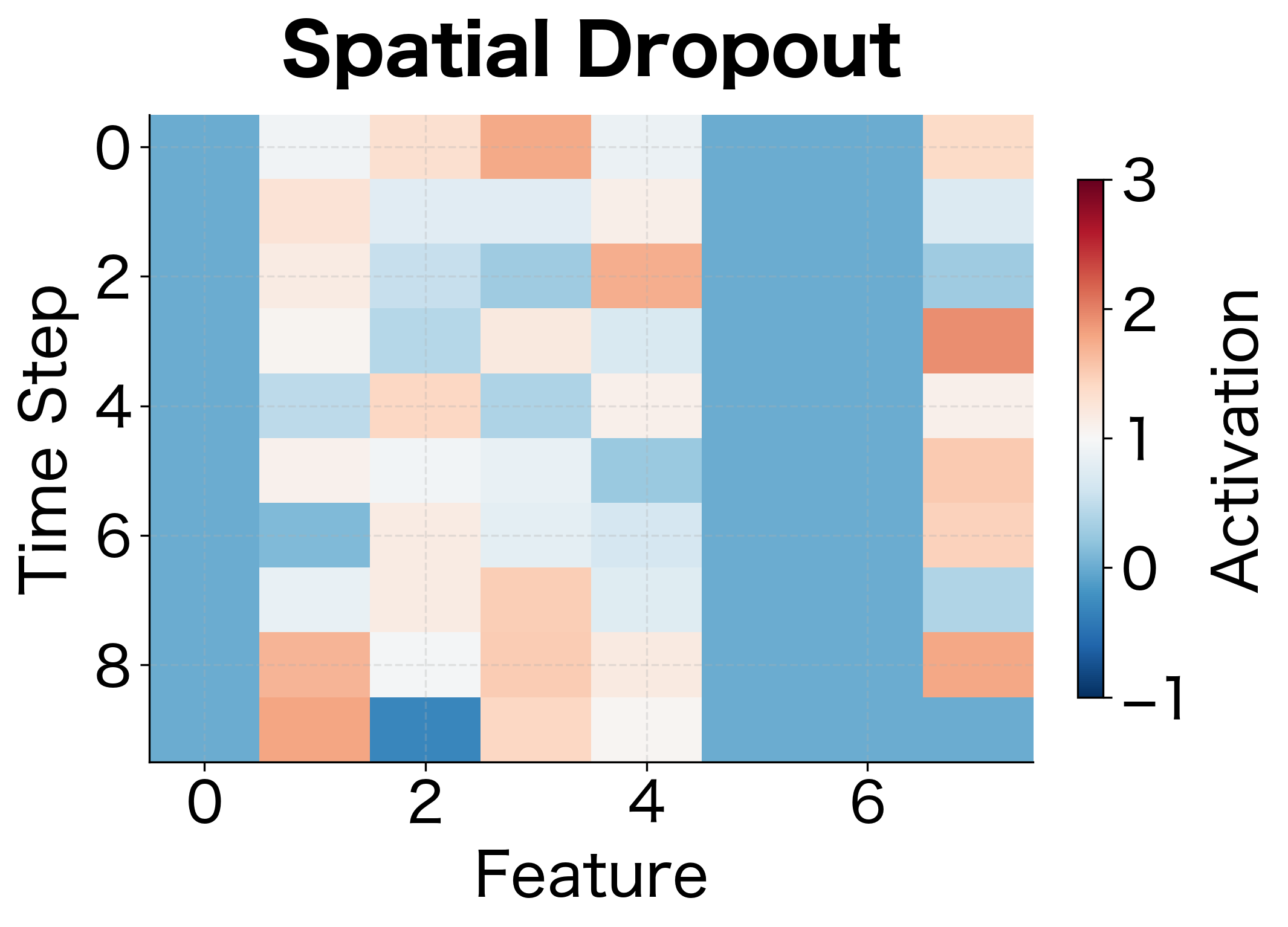
Spatial dropout is commonly used in convolutional neural networks (CNNs) and recurrent neural networks (RNNs). For language models processing sequences of embeddings, dropping entire embedding dimensions prevents co-adaptation between dimensions across the sequence.
Dropout in Modern Architectures
Dropout has evolved since its introduction. Modern architectures use it strategically, often in combination with other regularization techniques.
Dropout in Transformers
Transformers apply dropout in several places:
- Attention dropout: Applied to attention weights after softmax, before multiplying with values. This prevents the model from always attending to the same positions.
- Hidden layer dropout: Applied after the feed-forward sublayers.
- Embedding dropout: Sometimes applied to word embeddings.
- Residual dropout: Applied to sublayer outputs before adding to the residual connection.
DropConnect: A Variant
While standard dropout zeros activations, DropConnect zeros individual weights. Instead of , DropConnect computes:
where:
- : the output after DropConnect is applied
- : a binary mask matrix with the same shape as , where each element is independently sampled
- : the weight matrix connecting two layers
- : element-wise multiplication (Hadamard product)
- : the input to this layer
This provides a different form of regularization: the same input can produce different outputs because the effective weights change each forward pass. DropConnect regularizes at the weight level rather than the activation level, creating an even larger ensemble of possible sub-networks.
Dropout and Batch Normalization
An interesting interaction occurs when combining dropout with batch normalization. During training, dropout adds variance to activations, which batch normalization then tries to normalize away. This can lead to a train/test discrepancy because batch normalization uses running statistics at test time that were computed with dropout active.
Common practices include:
- Apply dropout after batch normalization
- Use lower dropout rates when using batch normalization
- Some architectures (like certain ResNets) omit dropout entirely when using extensive batch normalization
Code Implementation: Training with Dropout
Let's implement a complete training loop that uses dropout correctly. We'll train a simple network and compare its performance with and without dropout.
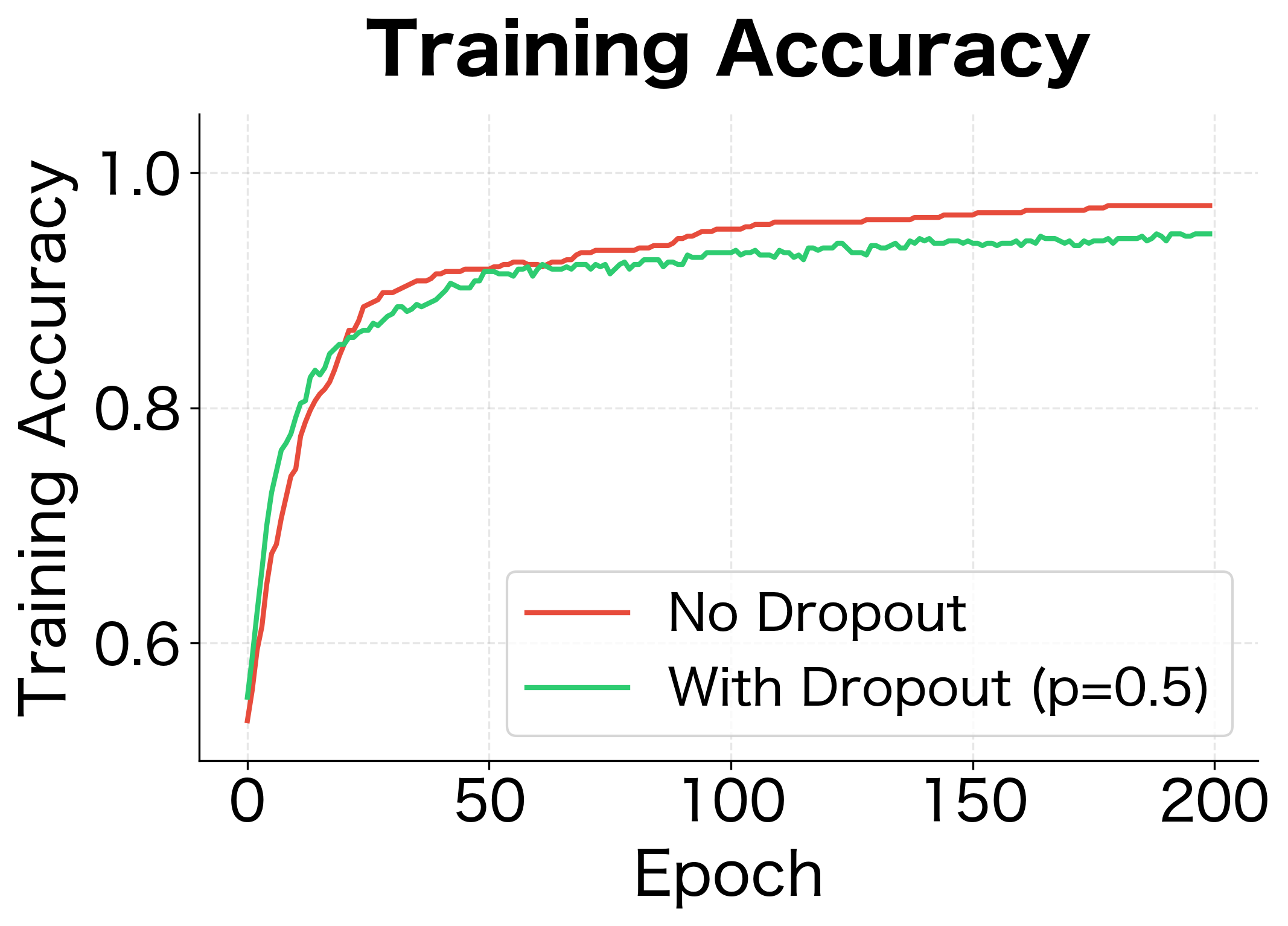
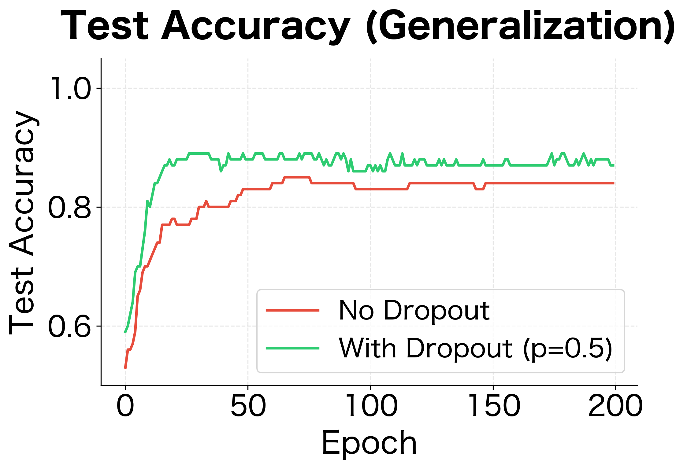
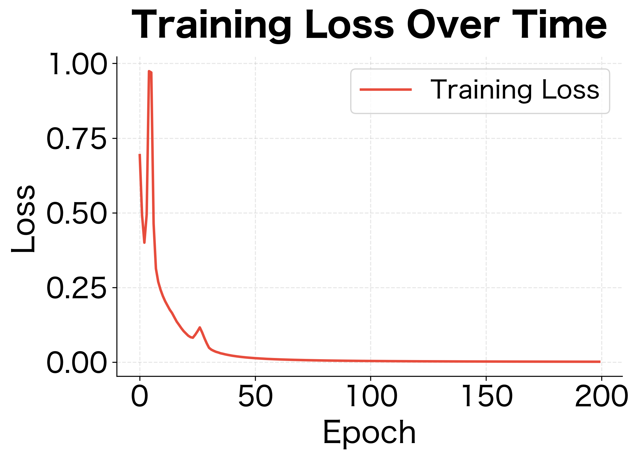
The results demonstrate dropout's regularization effect. Without dropout, the network achieves near-perfect training accuracy but poor test accuracy, a clear sign of overfitting. With dropout, training accuracy is lower but test accuracy is higher. The generalization gap (difference between train and test accuracy) shrinks significantly.
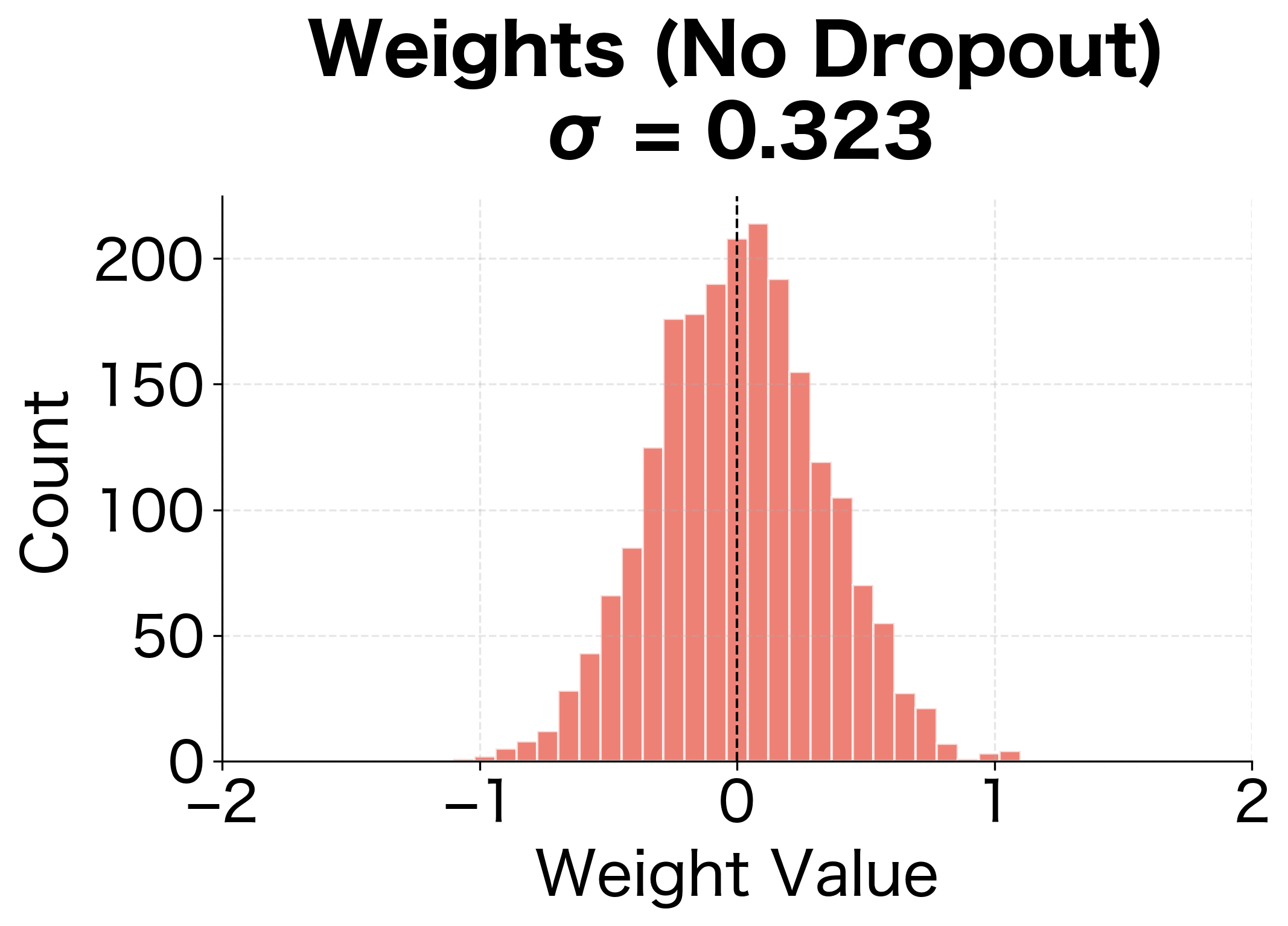
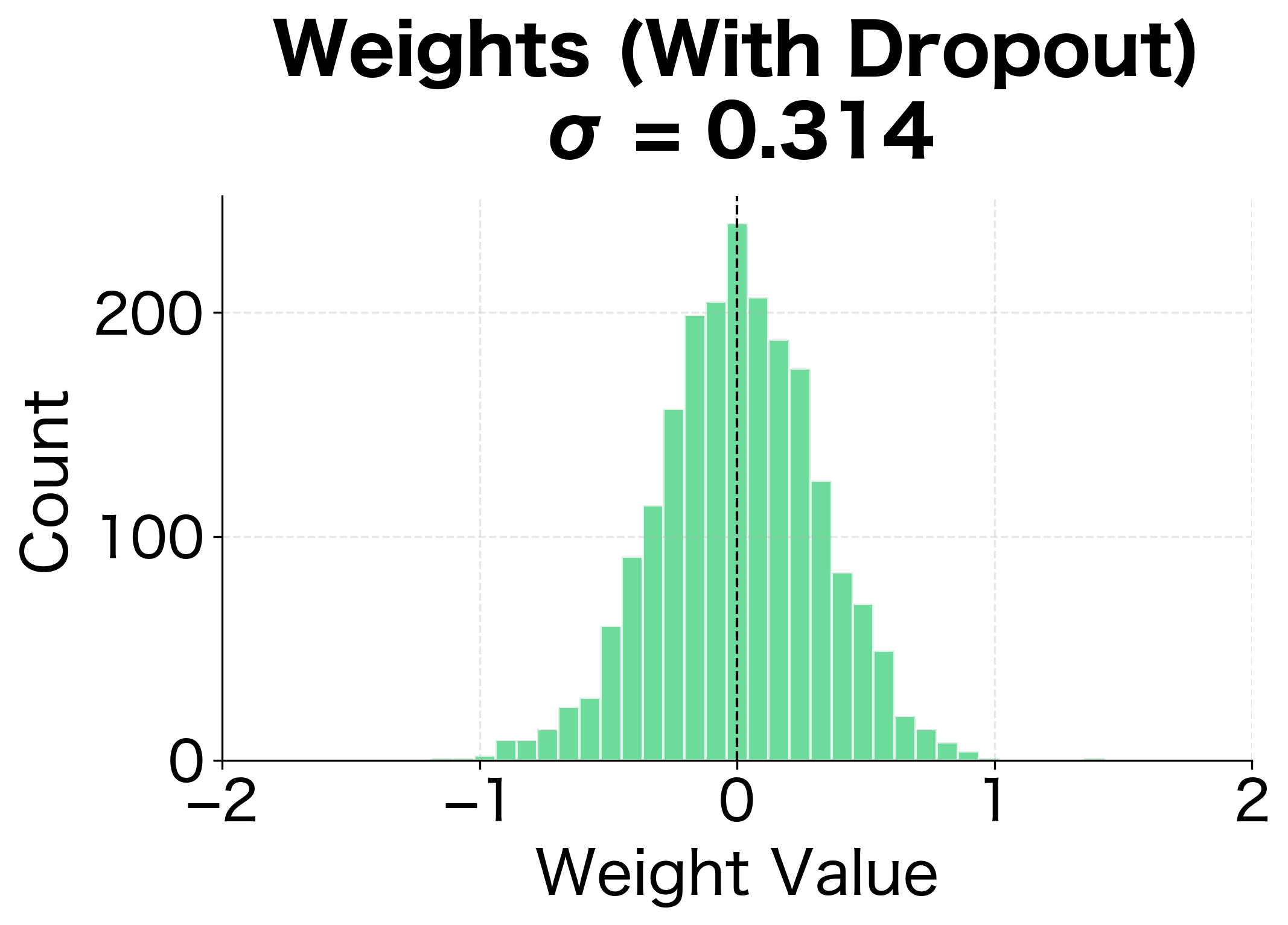
The weight distributions reveal another perspective on dropout's regularization effect. Without dropout, the network develops some larger weights as it memorizes specific training examples. With dropout, weights are more evenly distributed, suggesting the network has learned more distributed, redundant representations.
Limitations and Impact
Dropout transformed deep learning by providing a practical, effective regularization technique. However, it has important limitations that have driven the development of alternatives and variations.
Training time increases significantly. Because dropout effectively reduces the network's capacity during each forward pass, convergence is slower. The network must see more training examples to achieve the same level of learning. In practice, dropout can double or triple training time compared to an unregularized network.
Inference variability is a subtle issue. While inverted dropout ensures correct expected values, some applications require uncertainty estimates. Monte Carlo Dropout, running multiple forward passes with dropout enabled during inference, can provide uncertainty estimates but adds computational cost and implementation complexity.
Interaction with batch normalization is complex. As discussed earlier, the combination of dropout and batch normalization requires care. The variance injection from dropout during training doesn't match the batch normalization statistics computed for inference. Some modern architectures avoid this by using dropout sparingly or not at all when batch normalization is present.
Not all architectures benefit equally. Very deep networks with residual connections often find that careful initialization and batch normalization provide sufficient regularization. Dropout can sometimes hurt performance in these settings, particularly when applied too aggressively or in the wrong locations.
Despite these limitations, dropout had significant impact on the field. It demonstrated that noise injection during training could prevent overfitting without careful hand-tuning. This insight spawned a family of stochastic regularization techniques: DropConnect (dropping weights), DropPath (dropping entire residual branches), cutout (dropping input patches), and many others. The core principle, forcing redundancy through controlled randomness, remains influential in modern architecture design.
Summary
Dropout is a regularization technique that prevents overfitting by randomly setting neuron outputs to zero during training. The key insights from this chapter include:
-
Dropout trains an implicit ensemble. By randomly dropping neurons, we effectively train sub-networks that share weights. At test time, using all neurons approximates averaging their predictions.
-
Inverted dropout simplifies inference. By scaling activations by during training, we ensure the expected activation magnitude matches test time. This keeps inference code simple: just use all neurons without modification.
-
Dropout rate selection matters. The classic recommendation is for hidden layers and to for input layers. Modern practice often uses lower rates, especially when combined with other regularization.
-
Train/eval mode distinction is critical. Forgetting to disable dropout at inference time is a common bug. Always call
model.eval()before running predictions. -
Spatial dropout handles correlated features. For sequences and images, dropping entire feature channels (not individual neurons) provides more effective regularization by preventing information reconstruction from neighbors.
-
Modern architectures adapt dropout strategically. Transformers apply dropout to attention weights, hidden layers, and residual connections. The interaction with batch normalization requires care, leading some architectures to reduce or eliminate dropout.
Dropout's simplicity, just multiply by a random binary mask, belies its power. It remains one of the most widely used regularization techniques in deep learning, and its core insight about noise injection has influenced many subsequent developments in the field.
Key Parameters
When implementing dropout in neural networks, the following parameters directly affect model performance:
-
p(dropout rate): The probability of dropping each neuron. Common values are 0.5 for hidden layers and 0.1-0.2 for input layers. Higher values provide stronger regularization but slow convergence and can degrade performance if set too high. -
training(mode flag): Boolean indicating whether the model is in training or inference mode. During training, dropout is active; during inference, it must be disabled. Forgetting to switch modes is a common source of bugs. -
Dropout placement: Where dropout is applied in the network architecture matters. Apply after activation functions (not before), avoid the output layer, and be cautious when combining with batch normalization.
-
Spatial vs standard dropout: For sequential or spatial data, spatial dropout (dropping entire channels) is more effective than standard dropout because it prevents information reconstruction from correlated neighbors.
For PyTorch implementations, use nn.Dropout(p) for standard dropout and nn.Dropout1d(p) or nn.Dropout2d(p) for spatial dropout. The module automatically handles train/eval mode switching when you call model.train() or model.eval().
Quiz
Ready to test your understanding? Take this quick quiz to reinforce what you've learned about dropout regularization.

Comments