

Master linear classifiers including weighted voting, decision boundaries, sigmoid, softmax, and gradient descent. The building blocks of every neural network.

This article is part of the free-to-read Language AI Handbook
Choose your expertise level to adjust how many terms are explained. Beginners see more tooltips, experts see fewer to maintain reading flow. Hover over underlined terms for instant definitions.
Linear Classifiers
Before diving into the complex architectures of modern neural networks, we need to understand their fundamental building block: the linear classifier. This simple yet powerful model forms the core of every neuron in a deep network. Master this concept, and the rest of neural networks become variations on a theme.
Linear classifiers make predictions by computing a weighted combination of input features and comparing the result against a threshold. They draw straight lines (or hyperplanes in higher dimensions) to separate data into categories. While this simplicity limits what they can model, it also makes them fast, interpretable, and mathematically tractable, qualities that carry forward into the neural networks built upon them.
In this chapter, we'll build linear classifiers from the ground up. You'll learn how weights and biases define decision boundaries, why the dot product is the heart of the classification decision, and how gradient descent teaches the model to find good boundaries. We'll extend to multiclass problems with the softmax function and conclude by examining what linear classifiers cannot do, setting the stage for the neural networks that overcome these limitations.
The Core Idea: Weighted Voting
At its heart, a linear classifier is a voting system. Each input feature casts a vote, weighted by its importance, and the votes are summed to make a decision. Consider spam detection: certain words like "free" or "winner" should push the classification toward spam, while words like "meeting" or "quarterly" suggest legitimate email.
A linear classifier predicts a class based on a linear combination of input features. For input features , weights , and bias , the classifier computes and predicts the positive class if , otherwise the negative class.
Let's make this concrete with a simple example. Suppose we want to classify movie reviews as positive or negative based on word counts.
The scores reflect our intuition. Review 1, full of positive words, gets a high score. Review 2, dominated by negative words, scores low. Review 3 is close to zero, the decision boundary, reflecting its mixed nature. The weights encode which features matter and in which direction.
The Geometry: Decision Boundaries
Understanding linear classifiers geometrically reveals their power and limitations. In two dimensions, the classifier defines a line. Points on one side belong to class A; points on the other side belong to class B.
The equation defines the decision boundary: the set of all points where the classifier is perfectly undecided. The weight vector is perpendicular to this boundary and points toward the positive region. The bias shifts the boundary away from the origin.
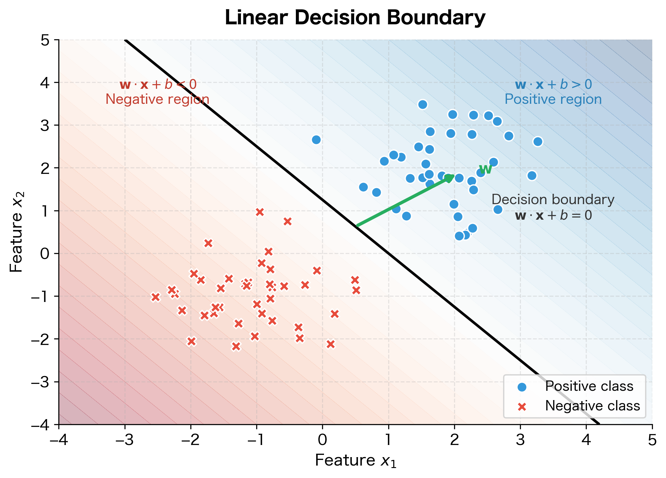
The color gradient shows the classifier's confidence: deeper blue indicates strong positive predictions, deeper red indicates strong negative predictions, and the transition occurs at the black decision boundary. Notice how the weight vector points perpendicular to the boundary, toward the positive (blue) region.
The Mathematics: Dot Products and Projections
We've seen that linear classifiers compute a score and use that score to make decisions. But what exactly does the dot product compute? Why is this particular operation the right choice for classification? Understanding the dot product from both algebraic and geometric perspectives reveals why linear classifiers work and what their limitations are.
The Algebraic Perspective: Weighted Voting
Start with the simplest view. The dot product computes a weighted sum: each input feature is multiplied by its corresponding weight, and the results are added together:
where:
- : the weight vector with components
- : the input feature vector with components
- : the weight for the -th feature (learned during training)
- : the value of the -th input feature
- : the number of features (dimensionality of the vectors)
Think of this as a voting system. Each feature casts a vote, and the weight determines how much that vote counts. A positive weight means "this feature provides evidence for the positive class," while a negative weight means "this feature provides evidence against." The magnitude of the weight reflects the feature's importance: a weight of 2.0 means this feature's vote counts twice as much as a feature with weight 1.0.
Consider spam detection with features like word counts. If "free" appears 5 times and has weight (suspicious), it contributes to the score. If "meeting" appears twice with weight (legitimate), it contributes . The final score aggregates all these votes into a single number that determines classification.
The Geometric Perspective: Measuring Alignment
The algebraic view tells us how to compute the dot product, but the geometric view tells us what it means. The dot product can equivalently be expressed as:
where:
- : the magnitude (length) of the weight vector
- : the magnitude of the input vector
- : the angle between the two vectors in -dimensional space
- : ranges from (opposite directions) to (same direction)
This formulation reveals the dot product's true nature: it measures how much points in the same direction as . The weight vector defines a "template" direction in feature space, and the dot product tells us how well each input matches that template.
When the vectors are perfectly aligned (), and the dot product reaches its maximum positive value. When they point in opposite directions (), and the dot product is maximally negative. When they're perpendicular (), and the dot product is exactly zero, meaning the input lies on the decision boundary.
This geometric insight explains why linear classifiers create straight decision boundaries: the set of points where (the decision boundary) consists of all vectors perpendicular to . In 2D, perpendicular vectors form a line; in 3D, a plane; in higher dimensions, a hyperplane.
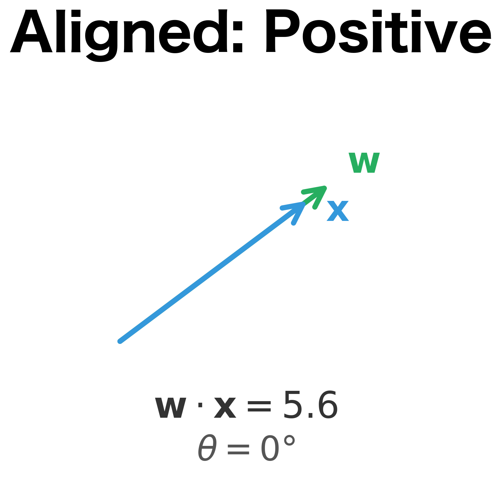
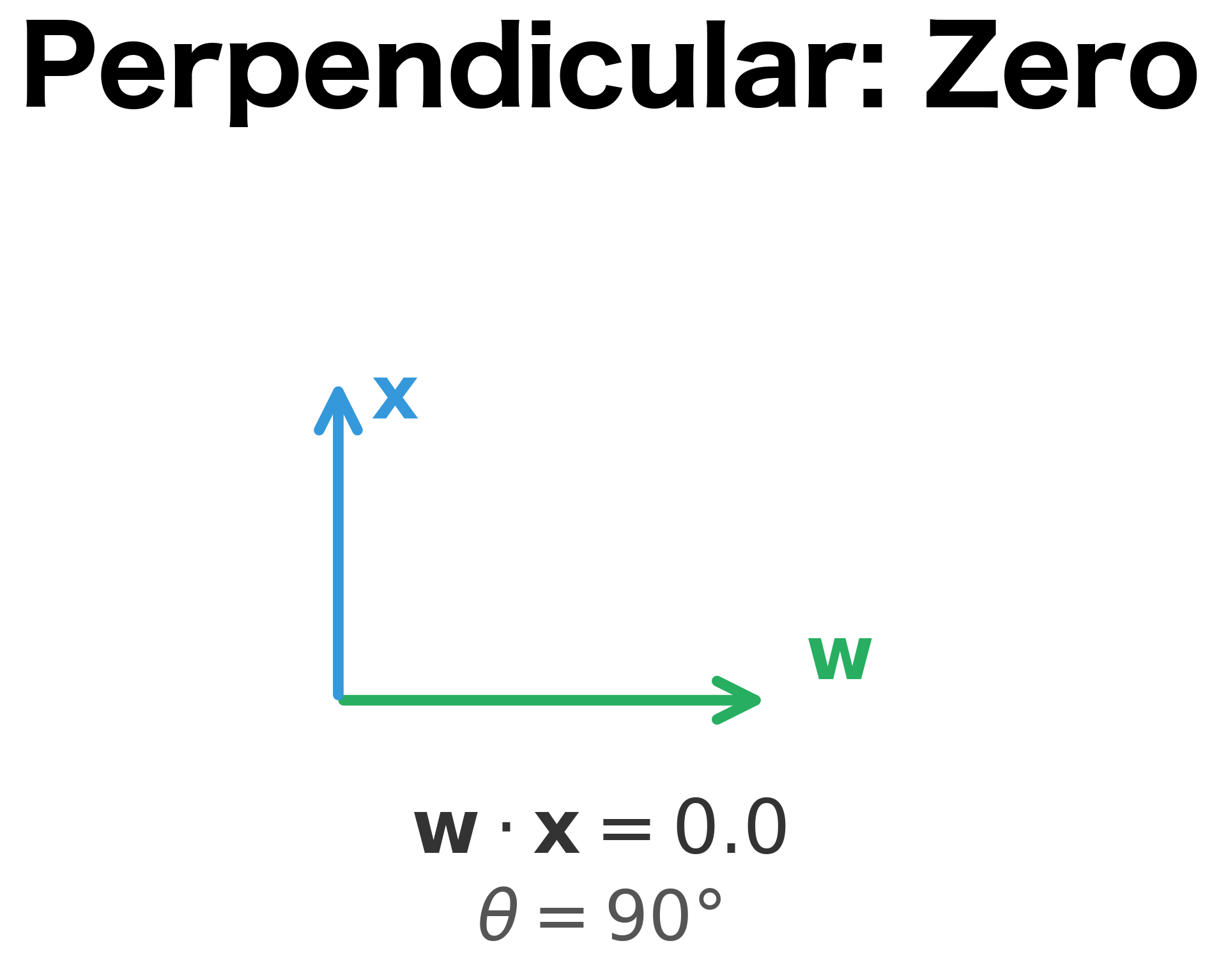
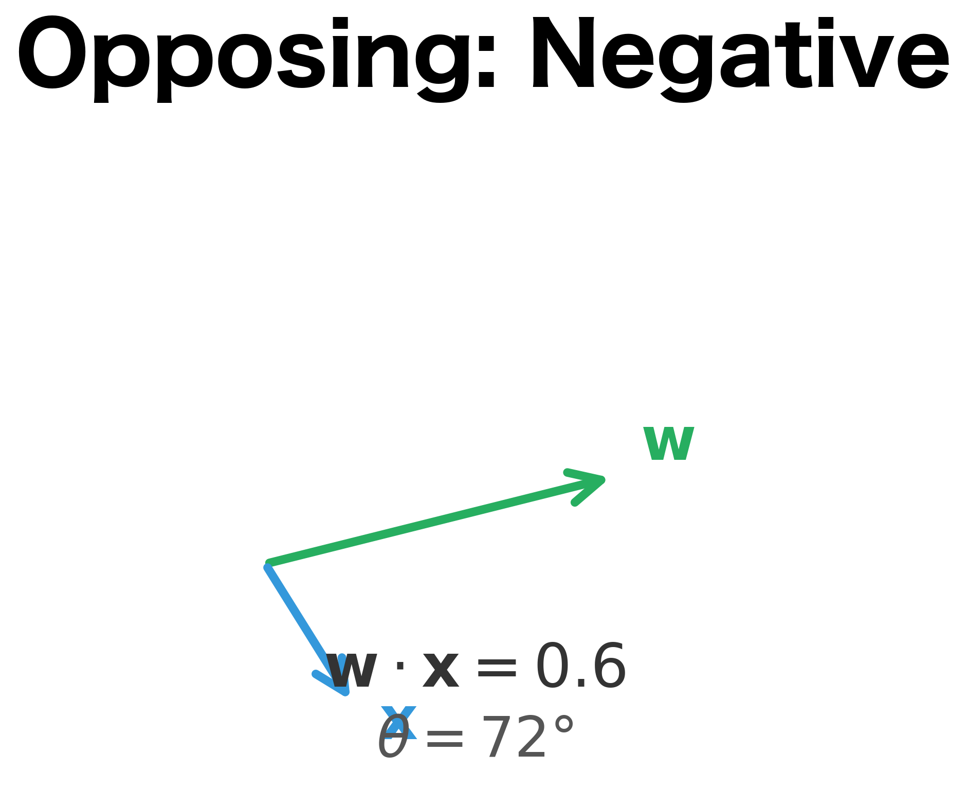
The visualization above makes this concrete. When the input vector aligns with the weight vector (left panel), the dot product is large and positive, indicating strong evidence for the positive class. When they're perpendicular (center), the dot product is zero, placing the input exactly on the decision boundary. When they oppose (right), the dot product is negative, indicating the negative class.
Binary Classification with Sigmoid
So far, we've treated the linear score as a direct decision: positive scores predict one class, negative scores predict another. But this binary output discards valuable information. A score of 0.01 (barely positive) and a score of 100 (strongly positive) both yield the same "positive" prediction, yet clearly we should be more confident about the second.
What we really want is a probability: a number between 0 and 1 that quantifies our confidence. This probability lets us make informed decisions: perhaps we flag emails as "suspicious" when but only auto-delete when .
The challenge is converting an unbounded score into a probability . We need a function that:
- Maps any real number to the interval
- Preserves order (higher scores → higher probabilities)
- Produces 0.5 when the score is 0 (maximum uncertainty)
- Approaches 1 for large positive scores and 0 for large negative scores
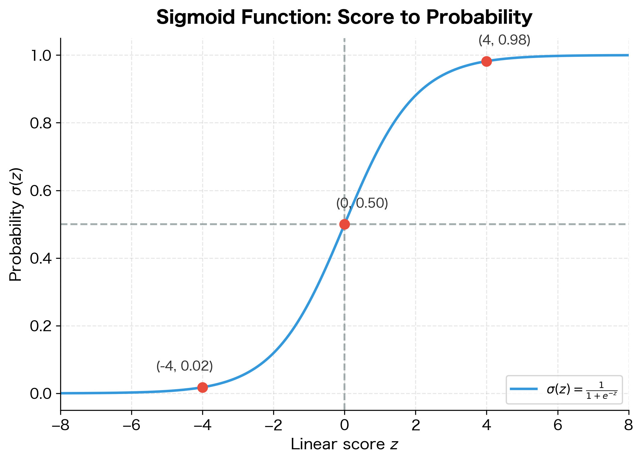
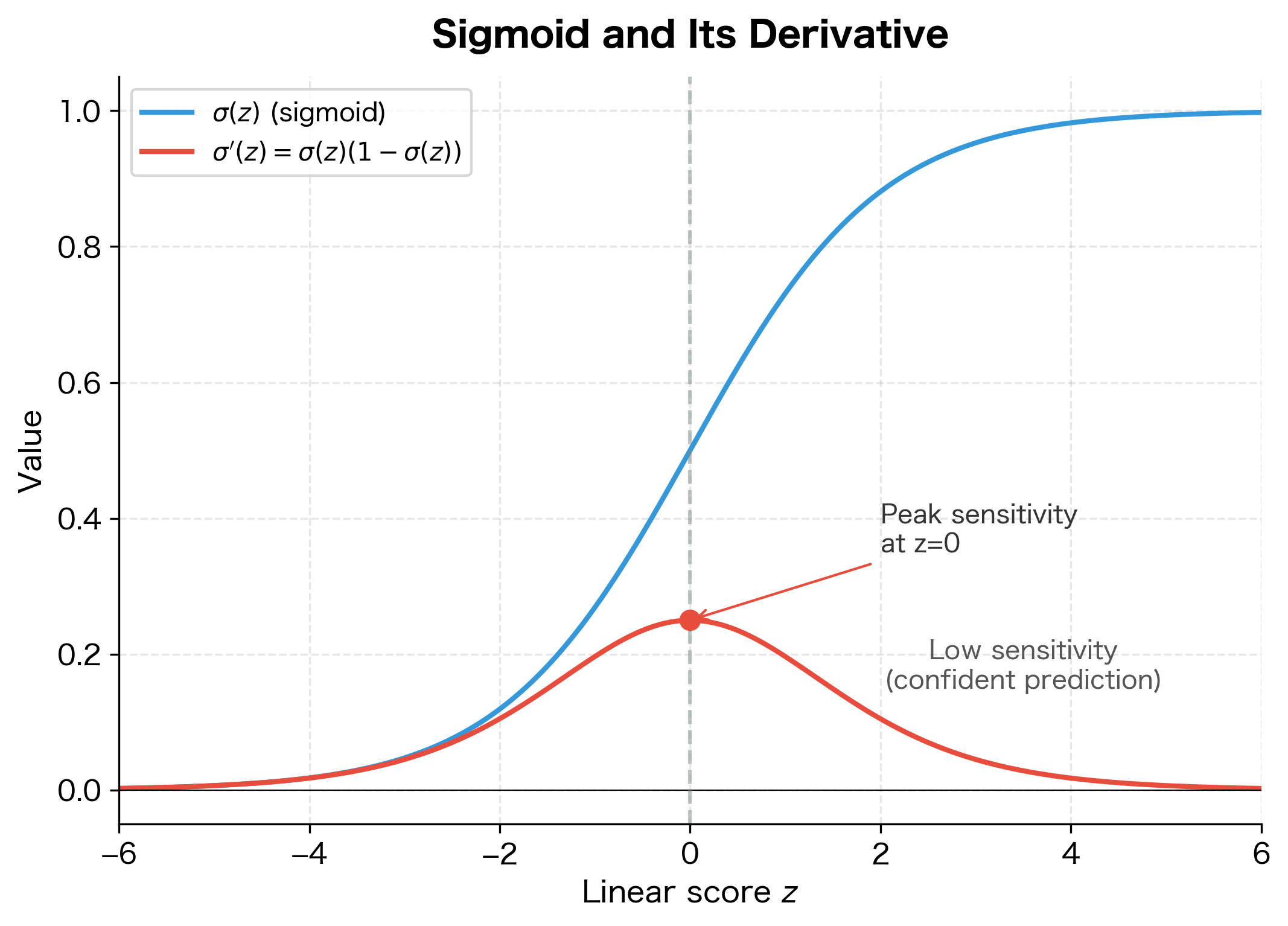
The sigmoid function satisfies all these requirements:
The sigmoid (or logistic) function maps any real number to the interval , making it suitable for interpreting scores as probabilities.
Why does this formula work? Consider what happens at extreme values. When is very large and positive, becomes tiny (approaching 0), so . When is very large and negative, becomes huge, so . At , we get , representing complete uncertainty.
The sigmoid has several useful properties:
- (uncertain prediction)
- As , (confident positive)
- As , (confident negative)
- Symmetric:
With the sigmoid, our classifier becomes a logistic regression model:
where:
- : probability of the positive class given input
- : the sigmoid function
- : weight vector
- : input feature vector
- : bias term
The probabilities give us richer information than hard predictions. Email 2 has only a 26% chance of being legitimate, a strong spam signal. Email 1 at 66% suggests legitimate but with some uncertainty, perhaps worth additional scrutiny.
Multiclass Classification with Softmax
Binary classification handles many problems, but what about distinguishing among three or more classes? Sentiment might be positive, negative, or neutral. A document might belong to sports, politics, technology, or entertainment. We need to extend our framework.
The natural approach: give each class its own weight vector and bias. An input gets separate scores, one per class:
But now we face a similar problem as before. These scores are unbounded real numbers. How do we convert scores into a probability distribution over classes?
We can't just apply sigmoid independently to each score, because that wouldn't guarantee the probabilities sum to 1. If sigmoid gives us and , we've created an impossible situation.
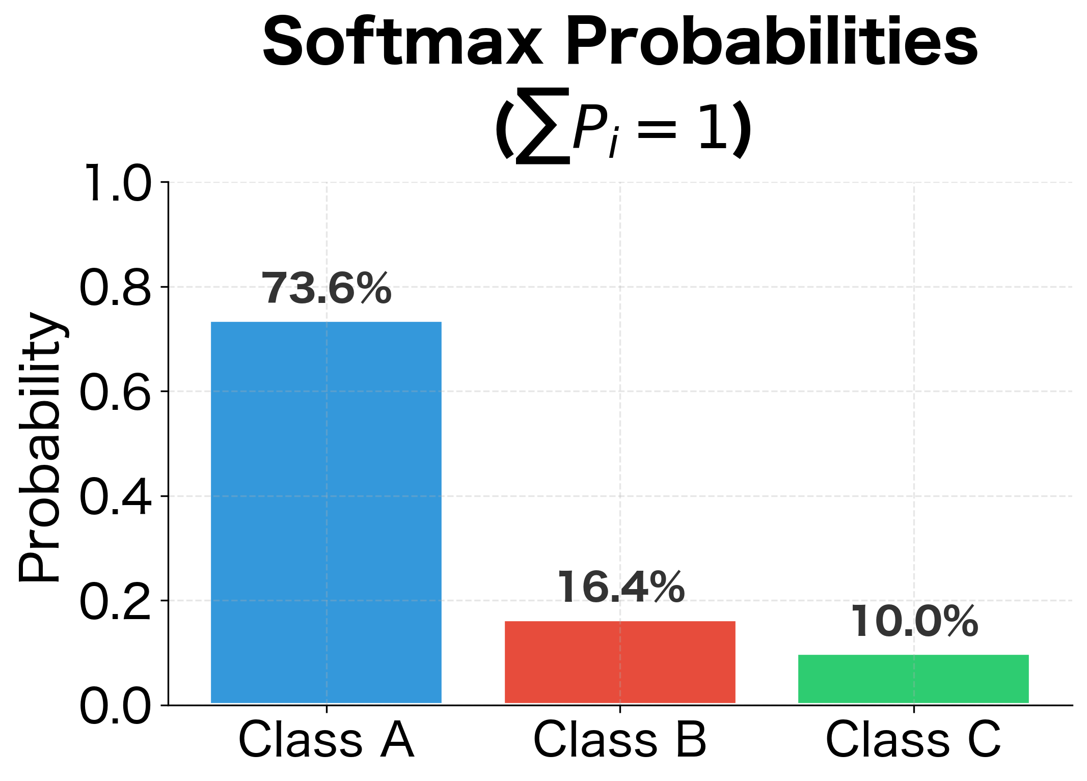
The solution is the softmax function, which explicitly enforces the constraint that probabilities sum to 1:
The softmax function converts a vector of real-valued scores (often called logits) into a probability distribution. For an input vector , the probability assigned to class is:
where:
- : the raw score (logit) for class
- : the exponential of , ensuring the value is positive
- : the sum of exponentials over all classes (normalization constant)
- : the total number of classes
The formula has an elegant structure. The numerator transforms the score into a positive number, with higher scores yielding larger values. The denominator sums these transformed scores across all classes, creating a normalization constant. Dividing by this sum guarantees the outputs sum to 1.
Why use the exponential function specifically? It has two key properties. First, it maps any real number to a positive value, ensuring valid probabilities. Second, it amplifies differences: if class A scores 3.0 and class B scores 1.0, the ratio of their softmax probabilities isn't 3:1 but rather , about 7:1. This amplification makes the winning class more decisive, which often matches our intuition that one class should dominate when its evidence is substantially stronger.
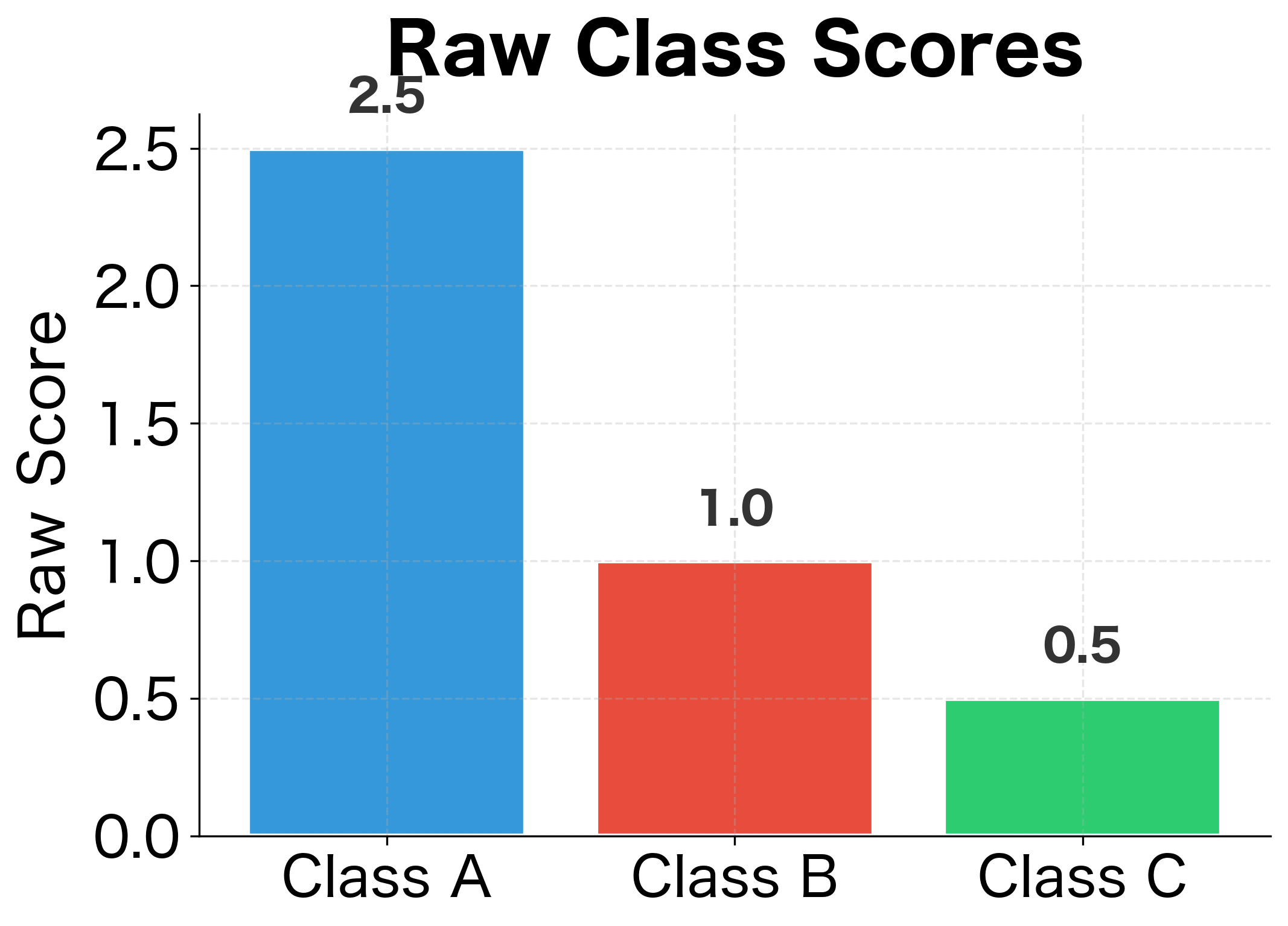
The table below compares three normalization approaches applied to the same raw scores. Notice how softmax amplifies the gap between classes compared to simple linear normalization:
| Class | Raw Score | Uniform | Linear (score/sum) | Softmax |
|---|---|---|---|---|
| A | 2.0 | 33.3% | 57.1% | 65.9% |
| B | 1.0 | 33.3% | 28.6% | 24.2% |
| C | 0.5 | 33.3% | 14.3% | 9.9% |
Notice how softmax handles competition between classes. In Review 1, the positive class dominates with 82.7% probability. In Review 3, the probabilities are more spread out, reflecting genuine ambiguity in the input.
Training with Gradient Descent
We've seen how linear classifiers make predictions, but we've been assuming the weights are already known. In practice, we start with random (or zero) weights and iteratively improve them based on training data. This learning process is gradient descent: computing how wrong our predictions are, then adjusting weights to reduce that error.
The key insight is treating learning as optimization. We define a loss function that measures how poorly the model performs, then systematically search for weights that minimize this loss. Gradient descent provides the search direction: at each step, we compute which direction makes the loss decrease fastest, then take a small step in that direction.
The Loss Function: Cross-Entropy
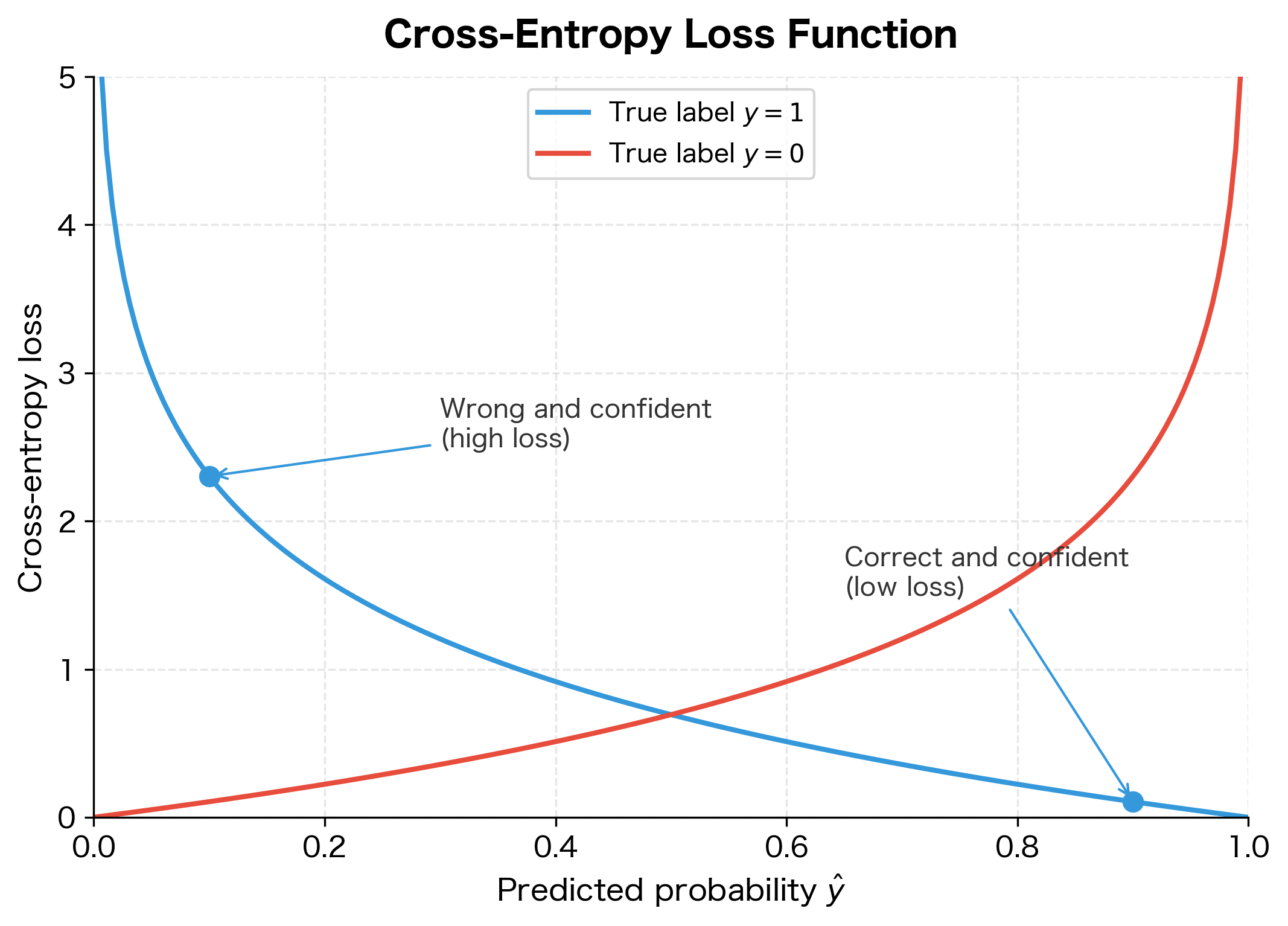
Before we can minimize anything, we need to define what "wrong" means mathematically. For classification, the standard choice is cross-entropy loss, also called log loss. This loss function has a crucial property: it penalizes confident wrong predictions far more severely than uncertain ones.
Consider what we want from a loss function. If the true label is "positive" and the model predicts 90% positive, that's good and should incur low loss. If the model predicts 10% positive for the same example, that's bad and should incur high loss. But critically, predicting 1% positive should be punished much more than predicting 40% positive, even though both are wrong. The 1% prediction is confidently wrong, while the 40% prediction at least shows appropriate uncertainty.
The cross-entropy loss achieves exactly this behavior. For a single binary example with true label and predicted probability :
where:
- : the loss value (lower is better, 0 is perfect)
- : the true label (either 0 or 1)
- : the predicted probability of class 1, output by the sigmoid function
- : natural logarithm (base )
- : contributes to loss only when (penalizes low )
- : contributes to loss only when (penalizes high )
The formula looks complicated, but it's actually two simpler cases combined. When the true label is , the term vanishes, leaving . When the true label is , the term vanishes, leaving .
Why the logarithm? The function has exactly the shape we need. When is close to 1, is close to 0, meaning low loss for correct confident predictions. As approaches 0, explodes toward infinity, severely punishing confident wrong predictions. The logarithm creates an asymmetric penalty structure that drives the model to be confident only when it's correct.
Think of it as measuring "surprise." If the model predicts and the true label is , the loss is : the model expected this outcome and isn't surprised. But if the model predicts for the same positive example, the loss is : the model is shocked by an outcome it considered unlikely.
Computing Gradients
With a loss function defined, we need to determine how to adjust each weight to reduce it. This is where the gradient enters: a vector pointing in the direction of steepest increase in loss. To minimize loss, we move in the opposite direction, taking steps proportional to the gradient's magnitude.
The gradient tells us: "If I increase by a tiny amount, how much does the loss change?" A positive gradient means increasing the weight would increase the loss, so we should decrease it instead. A negative gradient means increasing the weight would help, so we should increase it.
For logistic regression, deriving the gradient requires the chain rule from calculus. The computation flows through several intermediate quantities: the loss depends on the prediction , which depends on the score , which depends on the weights . We trace this chain step by step.
Step 1: Loss with respect to prediction. Starting from the cross-entropy loss , we differentiate with respect to :
This tells us how sensitive the loss is to changes in our prediction. When and is small (wrong prediction), is large and negative, indicating strong pressure to increase .
Step 2: Prediction with respect to score. The sigmoid function has a remarkably convenient derivative:
This derivative is always positive (since ), meaning increasing the score always increases the probability. It's largest when (where the model is most uncertain) and smallest near the extremes.
Step 3: Combining via chain rule. The chain rule multiplies these derivatives. After algebraic simplification (which is why sigmoid and cross-entropy are such a natural pairing), the result is surprisingly simple:
This is the prediction error: the difference between what the model predicted and what actually happened. When the model is correct (), the gradient is near zero and we barely update. When the model is wrong, the gradient is large and we update substantially.
Step 4: Score with respect to weights. Finally, since , we have and . Applying the chain rule once more:
where:
- : how much the loss changes when we slightly increase weight
- : how much the loss changes when we slightly increase the bias
- : the prediction error (difference between predicted probability and true label)
- : the -th input feature value
The final gradient has an elegant interpretation: it's the prediction error times the input feature. This makes intuitive sense. The error determines the magnitude of the correction: large errors mean large updates. The feature value determines which weights are responsible: if feature had value zero, it couldn't have contributed to the error, so its weight shouldn't change. If feature had a large value, it played a big role in the prediction, so its weight deserves a proportionally larger adjustment.
Let's train on a simple dataset and visualize how the decision boundary evolves:
The model converged to a solution with both weights positive and roughly equal, reflecting the symmetric nature of the data (both features contribute equally to separating the classes). The loss dropped by over 90% from its initial value, and the model achieves perfect classification on this linearly separable dataset.
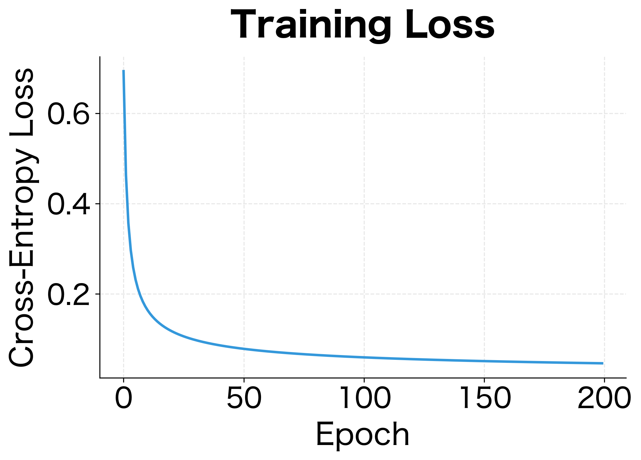
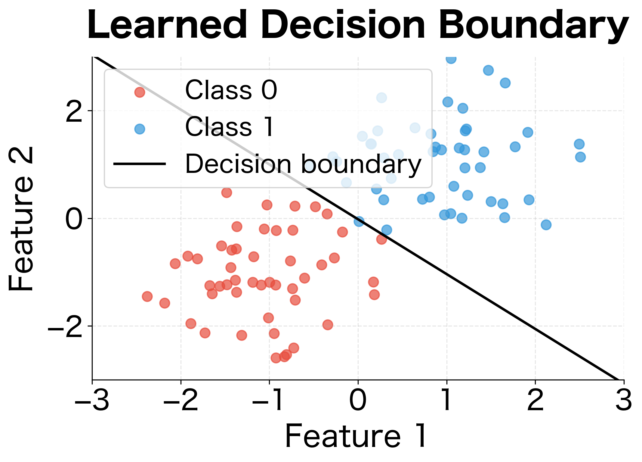
The training demonstrates gradient descent in action. The loss drops rapidly in early epochs as the model escapes its random initialization, then continues to decrease more slowly as it fine-tunes the boundary. The final decision boundary cleanly separates the two classes.
A Worked Example: Sentiment Classification
Let's bring everything together with a complete example: classifying movie reviews as positive or negative using a bag-of-words representation.
The classifier achieves perfect accuracy on the training set. The learned weights reveal which words the classifier associates with each sentiment: words like "wonderful," "fantastic," and "loved" receive positive weights, pushing predictions toward the positive class, while words like "worst," "terrible," and "boring" receive negative weights. This interpretability is a key advantage of linear classifiers.
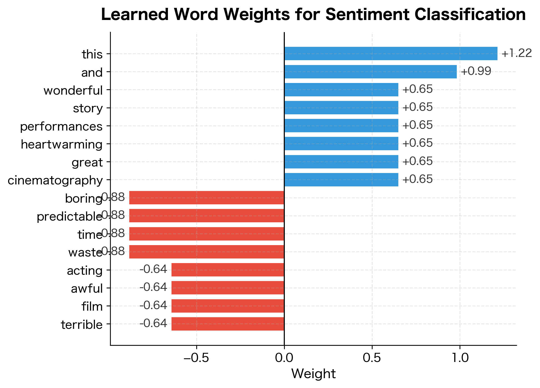
The classifier correctly identifies the first review as positive (high confidence due to "wonderful" and "fantastic") and the second as negative (due to "boring" and "terrible"). The third review contains no strongly weighted words from our training vocabulary, so it receives a probability near 50%, appropriately reflecting the model's uncertainty when it encounters unfamiliar language.
Limitations of Linear Classifiers
Linear classifiers are powerful, but their linearity imposes fundamental constraints. Understanding these limitations is crucial for knowing when to reach for more complex models.
The XOR Problem
The most famous limitation is the XOR problem. Consider data arranged such that positive examples are in the top-left and bottom-right quadrants, while negative examples are in the top-right and bottom-left. No single straight line can separate these classes.
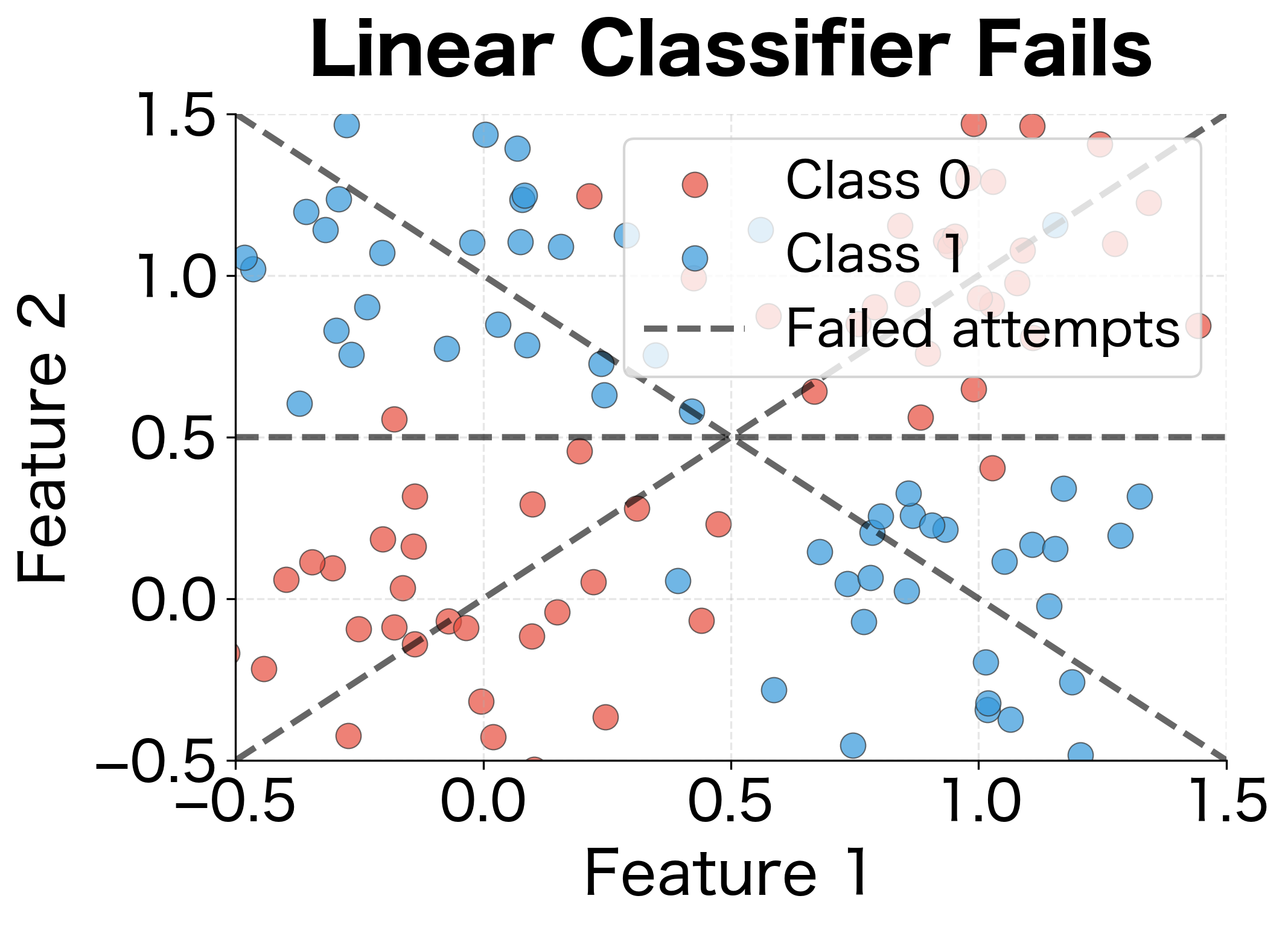
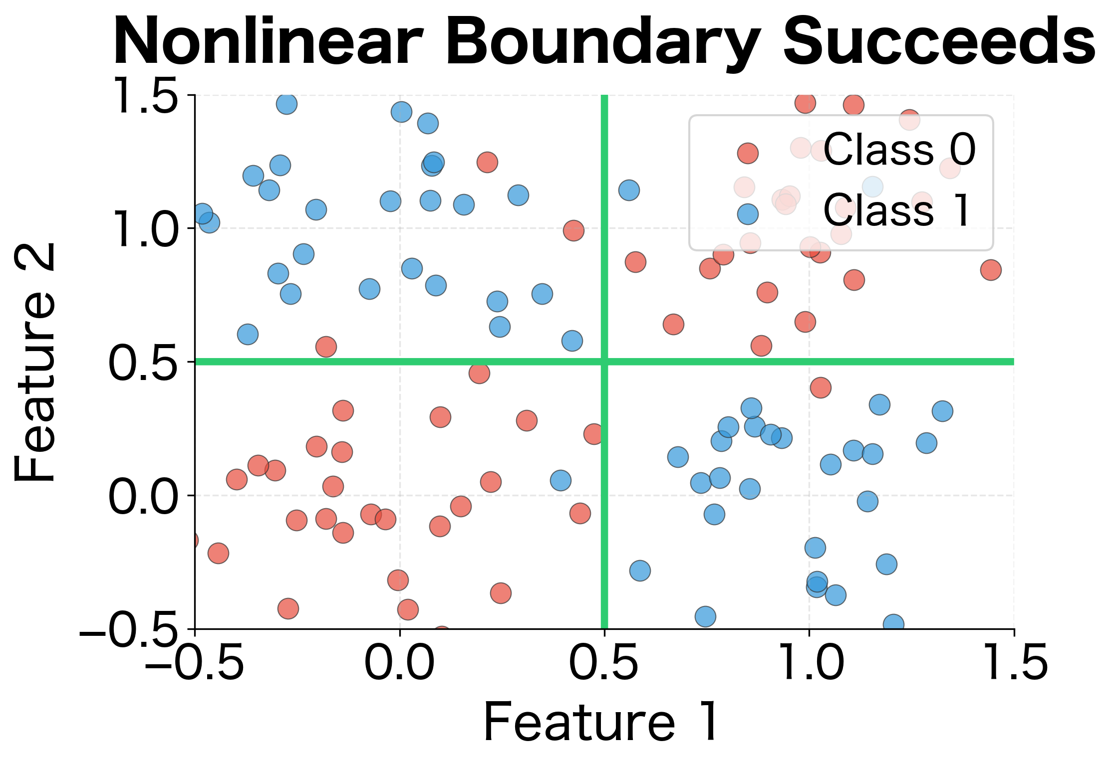
Curse of Feature Engineering
Before neural networks, practitioners addressed linear separability by manually engineering nonlinear features. For XOR, you might add a feature (the product of the two inputs), which makes the problem linearly separable in the expanded feature space.
But this approach doesn't scale. Real-world problems may require complex feature combinations that are impossible to discover manually. Consider image classification: which pixel products or transforms would help distinguish cats from dogs? The search space is astronomical.
What Linear Classifiers Unlock
Despite these limitations, linear classifiers remain foundational for several reasons:
-
Interpretability: The weights directly indicate feature importance. In spam detection, you can explain decisions: "This email was classified as spam because it contained 5 instances of 'free money.'"
-
Speed: Both training and inference are extremely fast. Matrix-vector multiplication is highly optimized on modern hardware.
-
Building blocks: Every neuron in a neural network is essentially a linear classifier followed by a nonlinear activation. Understanding linear classifiers is understanding the atoms of deep learning.
-
Surprising effectiveness: For many NLP tasks, especially with good features like TF-IDF or pretrained embeddings, linear classifiers achieve competitive performance. Sometimes the simplest model is good enough.
Key Parameters
When implementing linear classifiers and logistic regression, several parameters significantly impact model performance.
The key training parameters to tune are:
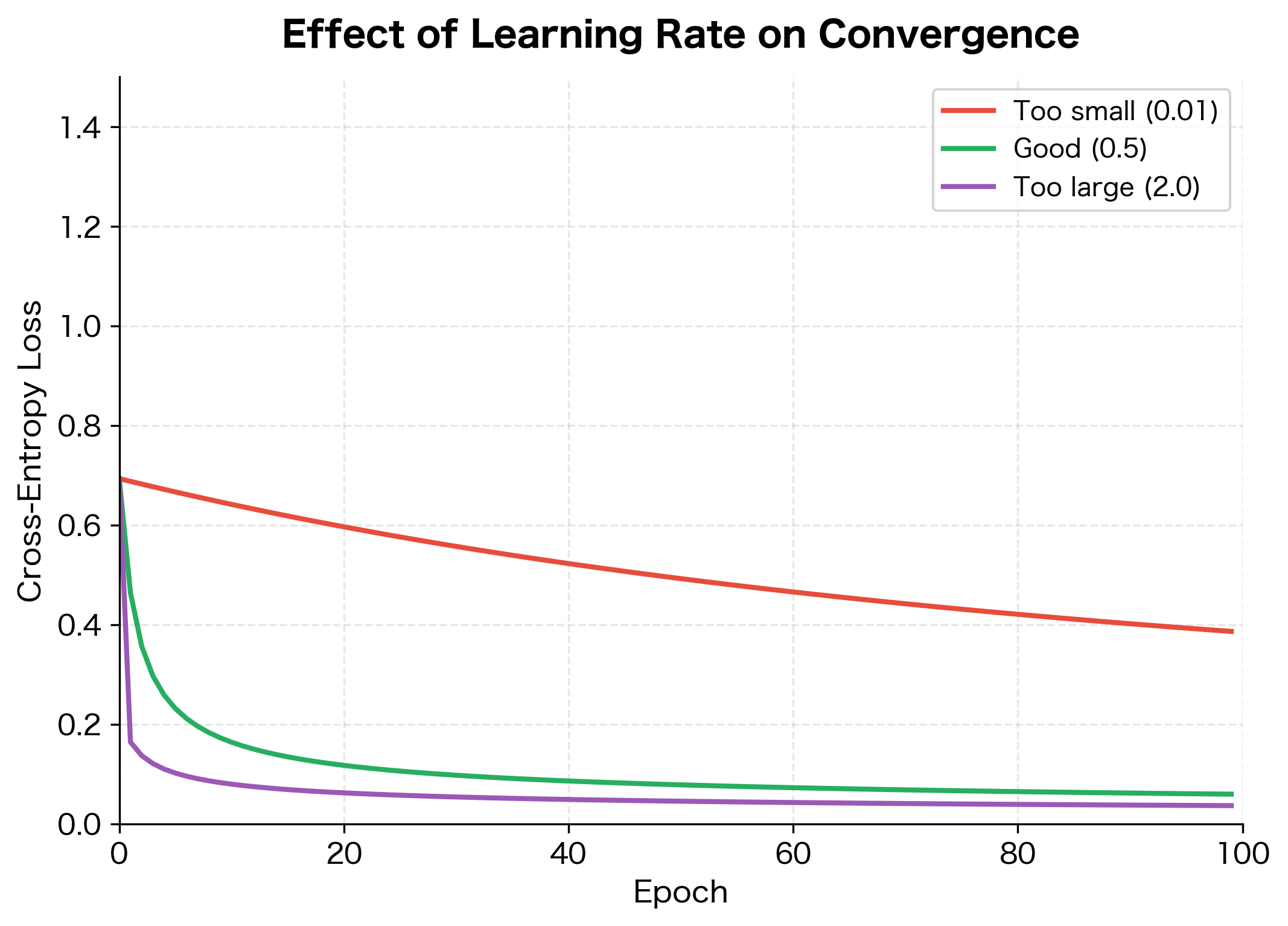
- learning_rate: Controls the step size during gradient descent. Too large causes oscillation or divergence; too small leads to slow convergence. Typical values range from 0.001 to 1.0. Start with 0.1 and adjust based on the loss curve behavior.
- n_epochs: Number of complete passes through the training data. More epochs allow the model to converge further, but excessive training on small datasets risks overfitting. Monitor the loss curve to determine when convergence occurs.
- Weight initialization: Initializing weights to zero (as in our implementation) works for linear classifiers since the loss landscape is convex. For neural networks, random initialization becomes essential.
- Regularization (not shown): Adding an L2 penalty term to the loss prevents overfitting by discouraging large weights. Common values for range from 0.0001 to 0.1.
- Numerical stability: The sigmoid and softmax functions can overflow or underflow with extreme inputs. Our implementation uses the max-subtraction trick for softmax and conditional computation for sigmoid to maintain numerical stability.
Summary
Linear classifiers form the foundation upon which neural networks are built. The key concepts from this chapter carry forward into every layer of a deep network:
Weighted voting: A linear classifier computes , where each feature votes according to its learned weight. This simple sum, followed by a threshold or nonlinearity, is the fundamental computation repeated billions of times in modern models.
Geometric intuition: The weight vector defines a decision boundary perpendicular to itself. Points are classified based on which side of this hyperplane they fall. The dot product measures alignment between input and weights.
Probabilistic interpretation: The sigmoid function transforms scores into probabilities, and the softmax extends this to multiple classes. These functions appear throughout neural networks wherever we need probability distributions.
Gradient descent: We train by computing gradients of the loss with respect to weights, then taking small steps in the opposite direction. The cross-entropy loss naturally pairs with sigmoid and softmax, giving simple gradient expressions.
Linear limitations: Some patterns, like XOR, cannot be separated by any linear boundary. This motivates the nonlinear activation functions and multiple layers of neural networks, which we explore in the next chapter.
You now have the vocabulary and intuition to understand what happens inside a neural network. Each layer performs linear classification, then breaks linearity with an activation function, then feeds forward to the next layer. The magic of deep learning emerges from stacking these simple operations.
Quiz
Ready to test your understanding? Take this quick quiz to reinforce what you've learned about linear classifiers, decision boundaries, and gradient descent.

Comments