

Master the Viterbi algorithm for finding optimal tag sequences in HMMs. Learn dynamic programming, backpointer tracking, log-space computation, and constrained decoding.

This article is part of the free-to-read Language AI Handbook
Choose your expertise level to adjust how many terms are explained. Beginners see more tooltips, experts see fewer to maintain reading flow. Hover over underlined terms for instant definitions.
Viterbi Algorithm
When labeling a sequence of tokens, you face a fundamental decision: should you choose each label independently, or should you consider the entire sequence at once? Greedy decoding picks the best label at each position, ignoring how earlier choices affect later ones. But sequence labeling isn't about finding locally optimal tags; it's about finding the globally optimal tag sequence.
The Viterbi algorithm solves this problem elegantly. Given a sequence of observations and a model that defines transition and emission probabilities, Viterbi finds the single best sequence of hidden states. For part-of-speech tagging, it finds the best tag sequence. For named entity recognition, it finds the best BIO label sequence. The algorithm runs in time linear in the sequence length, making it practical for real applications.
This chapter develops the Viterbi algorithm from first principles. You'll understand why exhaustive search is intractable, how dynamic programming makes the problem solvable, and how to implement efficient decoding in practice. We also explore log-space computation to avoid numerical underflow and show how Viterbi forms the foundation for beam search decoding in neural sequence models.
The Optimal Path Problem
Consider a hidden Markov model for part-of-speech tagging. You observe a sequence of words and want to find the sequence of tags that maximizes the joint probability of seeing both the tags and the words together. The HMM factors this joint probability into a product of simpler terms:
where:
- : the sequence of hidden states (POS tags) we want to infer
- : the observed sequence of words
- : the initial state probability, capturing how likely the sentence starts with tag
- : the transition probability from tag to tag , encoding grammatical patterns like "determiners often precede nouns"
- : the emission probability of word given tag , capturing which words are typical for each tag
The first product captures transition probabilities: how likely is each tag given the previous one? The second product captures emission probabilities: how likely is each word given its tag? This factorization embodies the Markov assumption: each tag depends only on its immediate predecessor, not on the full history.
Given a sequence of observations and a model with transition and emission probabilities, find the sequence of hidden states that maximizes the probability of generating those observations.
Why Greedy Decoding Fails
A greedy approach picks the best tag at each position independently, considering only the previous tag. At each position , greedy decoding selects:
where:
- : the greedily chosen tag at position
- : selects the tag that maximizes the following expression
- : the emission probability of the current word given candidate tag
- : the transition probability from the previously chosen tag to candidate tag
This seems reasonable but can produce suboptimal sequences. The problem is that a locally good choice might force bad choices later. Consider tagging "The can can hold water." A greedy tagger might assign MODAL to the first "can" because modals are common after determiners. But this makes the second "can" difficult: modals rarely follow modals. The globally optimal solution assigns NOUN to the first "can" and VERB to the second, even though NOUN isn't the highest-probability tag for "can" in isolation.
This example demonstrates why greedy decoding fails. The locally optimal choice of MD for the first "can" yields score 0.180, beating NN's 0.125. But this decision creates a problem: the second "can" must follow a modal, and modals rarely follow modals (P(MD|MD) = 0.05). The alternative path through NN enables a much higher score at the next position (0.060 vs 0.030), potentially yielding a better overall sequence probability.
Let's trace the cumulative scores for both paths:
| Position | Greedy Path (DT→MD→VB) | Alternative Path (DT→NN→VB) |
|---|---|---|
| Position 2 (first "can") | 0.180 | 0.125 |
| Position 3 (second "can") | 0.0216 | 0.0075 |
The greedy path starts stronger (0.180 vs 0.125) because MD has higher emission probability for "can." But this local advantage creates a problem: the MD→VB transition at position 3 yields only 0.0216, while NN→VB would have enabled a score of 0.0075. The globally optimal path requires looking ahead, something greedy decoding cannot do.
The Exponential Search Space
If greedy decoding doesn't work, why not try all possible tag sequences? With possible tags and a sequence of length , there are possible sequences. For a modest vocabulary of 45 tags and a 20-word sentence, that's sequences, far more than the number of atoms in the observable universe.
Even with a modest 45-tag vocabulary, a 20-word sentence produces more possible sequences than atoms in the observable universe. Checking each sequence individually would take longer than the age of the universe on any computer. The key insight is that we don't need to enumerate every sequence. Many sequences share common prefixes, and we can avoid recomputing scores for these shared subsequences. This is where dynamic programming enters.
The Viterbi Recursion
We've established that greedy decoding fails because local choices can force globally suboptimal sequences, and that exhaustive search is computationally impossible. How can we find the optimal path without examining every possibility? The answer lies in a beautiful insight from dynamic programming: we can build the optimal solution incrementally from smaller optimal solutions.
The Key Insight: Optimal Substructure
Imagine you're at position 3 in a sequence, and you want to know the best path that ends at the tag NOUN. Here's the crucial observation: regardless of how that path reached position 2, the best continuation to NOUN at position 3 depends only on:
- What state we're in at position 2 (not how we got there)
- The transition probability to NOUN
- The emission probability of the observed word from NOUN
This property is called optimal substructure. If the best path through the entire sequence passes through state at position 2 and then reaches NOUN at position 3, then the portion of that path from the start to must itself be optimal. Why? If there were a better path to , we could substitute it and get a better overall path, contradicting our assumption that we had the best path.
The best path ending at state at position consists of the best path to some state at position , followed by a transition from to . We can find the globally optimal path by computing locally optimal subpaths.
This principle transforms our approach entirely. Instead of tracking complete paths (exponentially many), we only need to track the best score for reaching each state at each position. At any position, we have just values to maintain, one per possible state, rather than an exponentially growing set of paths.
Building the Recurrence: From Intuition to Formula
Let's formalize this insight. We define as the probability of the most likely path that:
- Ends at state at position
- Generates the observations seen so far
How do we compute ? Consider any path ending at state at position . That path must have come from some predecessor state at position . The probability of this path factors into three terms:
- The probability of the best path to : This is , which we've already computed
- The transition probability from to : This is
- The probability of emitting the current observation from : This is
Since we want the best path to , we take the maximum over all possible predecessor states. This gives us the Viterbi recurrence:
where:
- : the probability of the best path ending at state at position
- : takes the maximum over all possible predecessor states
- : the best score for reaching state at the previous position (already computed)
- : the transition probability from predecessor state to current state
- : the emission probability of observing word from state
Notice that appears inside the maximization but doesn't depend on the predecessor . This is because once we decide to be in state at position , the emission probability is fixed regardless of how we arrived. We could factor it out:
This form is computationally equivalent but makes clear that we're choosing the best predecessor based solely on the accumulated path score and transition, then multiplying by the emission.
The Base Case: Starting the Sequence
The recurrence needs a starting point. At position 1, there is no predecessor to consider. The probability of the best path ending at state after seeing just the first observation is simply:
where:
- : the initial state probability (how likely the sequence starts in state )
- : the emission probability of the first observation from state
This captures both how likely we are to start in state and how well state explains the first observed word.
Complexity: Why This Works
Let's count the operations. At each of the positions (after the first), we compute for each of the states. Computing each requires examining predecessors. Total: operations.
Compare this to the paths we would examine exhaustively:
| Approach | Complexity | 45 tags, 20 words |
|---|---|---|
| Exhaustive | ~ | |
| Viterbi | 40,500 |
The exponential has become polynomial. This is the power of dynamic programming: by recognizing that we can solve the problem incrementally and that we only need to remember the best score per state (not every path), we collapse an intractable problem into an efficient algorithm.
Visualizing the Trellis
It helps to visualize the Viterbi computation as filling a grid called a trellis. The horizontal axis represents positions in the sequence (1 through ), and the vertical axis represents possible states (the tags or labels). Each cell holds the score , the probability of the best path ending at state at position .
Arrows connect cells at adjacent positions. Each arrow from to represents one term in the maximization: "if I came from state , what would my score be?" The algorithm fills this grid column by column, left to right, computing each cell from the cells in the previous column.
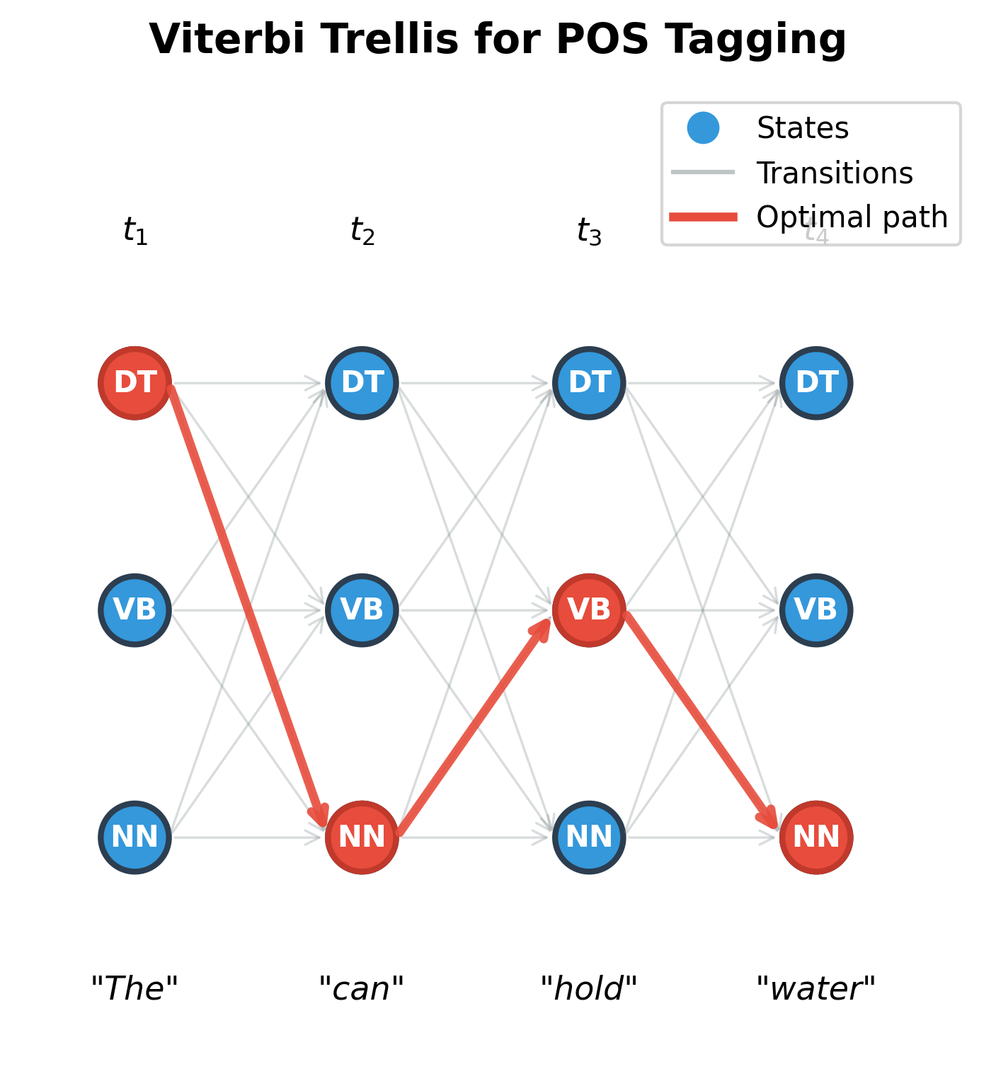
In the figure above, gray arrows show all possible transitions between adjacent positions. The red path highlights the optimal sequence discovered by Viterbi: DT → NN → VB → NN for the sentence "The can hold water." Notice that:
- At position 1, DT (determiner) wins because "The" is overwhelmingly a determiner
- At position 2, NN (noun) wins, not because "can" is most often a noun, but because this choice enables better continuations
- The algorithm found this globally optimal path without explicitly enumerating all 81 possible sequences (3 states × 4 positions)
Now we understand how Viterbi computes scores efficiently. But there's a missing piece: at the end of the algorithm, we know the score of the best path, but we haven't recorded the path itself. How do we reconstruct which states we actually passed through?
Backpointer Tracking
The Viterbi recurrence gives us the score of the best path to each state, but we've lost something in the process: which path achieved that score? At each step, we took the maximum over predecessors, keeping only the winning score. To reconstruct the actual optimal sequence, we need to remember which predecessor won at each cell.
The Need for Backpointers
Think of it this way: when we compute , we're answering "what's the best path probability ending at NOUN at position 3?" But we're not recording "and that path came through VERB at position 2." Without this information, when we finish computing the entire trellis, we'll know that the best final state is (say) NOUN with score 0.0073, but we won't know the sequence of states that led there.
The solution is elegantly simple: alongside each score, store the predecessor that achieved it. We call this a backpointer because it points backward to the previous state in the optimal path.
Formalizing Backpointers
The backpointer records which predecessor state maximized the score when computing :
where:
- : the backpointer for state at position , storing which predecessor led to the best score
- : returns the state (not the value) that maximizes the expression
- The expression inside is identical to the Viterbi recurrence
Notice the difference between and :
- returns the value: "the best score is 0.042"
- returns the argument: "the best predecessor is VERB"
We compute both simultaneously: the same computation that finds the maximum score also identifies which predecessor achieved it.
Reconstructing the Path: The Backward Pass
Once we've filled the entire trellis, we have scores and backpointers for every (position, state) pair. Reconstruction proceeds in three steps:
Step 1: Find the best final state. The optimal path ends at whichever state has the highest score at the final position:
where:
- : the optimal state at the final position
- : the Viterbi score at the final position for each state
Step 2: Follow backpointers backward. Starting from , we trace back through the stored pointers:
where:
- : the optimal state at position
- : the backpointer stored at position for state , which tells us which state at position led to the best path through
Each backpointer tells us: "to reach this state optimally, I came from that state." By following this chain, we recover the complete path.
Step 3: Reverse the sequence. Since we traced from position back to position 1, the recovered sequence is in reverse order. A simple reversal gives us the forward path.
Why Backpointers Work
The beauty of this approach is that backpointers require only additional storage, one pointer per cell in the trellis, and add no complexity to the forward pass (we're already examining all predecessors to compute the maximum). The backward pass is a simple traversal.
Reading the Implementation
Let's walk through how this code implements the formulas we developed:
-
Initialization (lines 17-24): We create two data structures:
Vfor Viterbi scores andbackpointerfor tracking predecessors. Each is a list of dictionaries, one per position. -
Base case (lines 26-30): For the first observation, we apply . There's no predecessor, so backpointers are
None. -
Recursion (lines 32-50): The nested loops implement the recurrence. For each position
iand each states, we examine all predecessorss_prev, compute the score , and keep the maximum. We store both the score (V[i][s]) and which predecessor achieved it (backpointer[i][s]). -
Termination and backtracking (lines 52-63): We find the state with the highest final score (this is ), then follow backpointers backward to reconstruct the path.
The implementation uses a small epsilon (1e-10) instead of zero for missing probabilities to avoid numerical issues with exact zeros.
A Worked Example
Now let's trace through this algorithm on a concrete problem. We'll use a simple HMM for weather inference: given a sequence of observed activities (walking, shopping, cleaning), infer the most likely sequence of weather states (sunny or rainy).
The HMM parameters encode two types of knowledge about the weather-activity relationship:
Transition Probabilities : How likely is each weather state given the previous day's weather?
| Current State | → Sunny | → Rainy |
|---|---|---|
| Sunny | 0.7 | 0.3 |
| Rainy | 0.4 | 0.6 |
Emission Probabilities : How likely is each activity given the current weather?
| Weather State | walk | shop | clean |
|---|---|---|---|
| Sunny | 0.6 | 0.3 | 0.1 |
| Rainy | 0.1 | 0.4 | 0.5 |
These tables reveal the model's structure. Weather tends to persist: sunny days have 70% chance of staying sunny, rainy days 60% chance of staying rainy. For activities, walking is a strong indicator of sunny weather, while cleaning suggests rain. Shopping is the most ambiguous activity, slightly favoring rainy days.
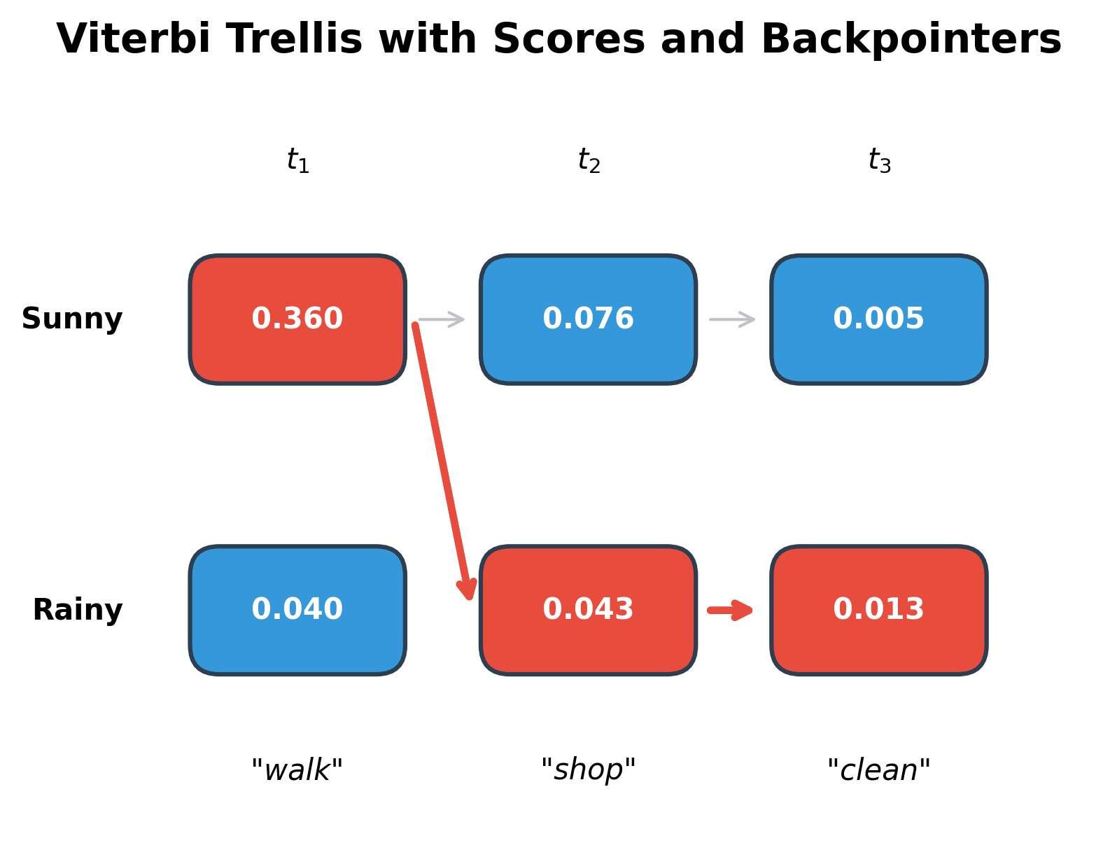
Let's interpret this step-by-step computation:
Position 0 (observing "walk"): We apply the base case formula . Sunny scores higher (0.360 vs 0.040) for two reinforcing reasons: the prior favors sunny days (0.6 vs 0.4), and walking is much more likely on sunny days (0.6 vs 0.1).
Position 1 (observing "shop"): Now the recurrence kicks in. For each current state, we consider both possible predecessors:
- To reach Sunny: the best predecessor is Sunny (score 0.0756), since we benefit from both the high previous score and a favorable transition (sunny days tend to stay sunny)
- To reach Rainy: again the best predecessor is Sunny (score 0.0432), despite the transition penalty, because the previous Sunny score was so much higher than Rainy
The result: The optimal path Sunny → Sunny → Rainy aligns with intuition: walking strongly suggests good weather, shopping is ambiguous (slightly favoring rain), and cleaning strongly suggests rain. The algorithm found this without examining all 8 possible paths. It computed only 12 values (2 states × 3 positions × 2 predecessor checks).
Log-Space Computation
Multiplying many small probabilities causes numerical underflow. For a sequence of 100 tokens with probabilities around 0.01, the path probability would be approximately , far below the smallest representable floating-point number (approximately for 64-bit floats).
The solution is to work in log space. The logarithm function has a useful property: it converts products into sums. Since , we can rewrite the Viterbi recurrence entirely in terms of log probabilities:
where:
- : the log probability of the best path ending at state at position
- : the log probability of the best path to predecessor state (already computed)
- : the log transition probability from to
- : the log emission probability of word from state
Log probabilities are negative since probabilities are between 0 and 1, and when . The best path has the highest (least negative) log probability. The operation is unchanged because log is monotonic: if , then . This means finding the maximum log probability gives the same answer as finding the maximum probability.
Both methods find the identical optimal path, confirming that log-space computation preserves correctness. The probability-space result (best_prob) and the exponentiated log-space result match to numerical precision. For the 100-token demonstration, probability space underflows to exactly zero while log space produces a meaningful value of -230.26. This is why all production Viterbi implementations work in log space.
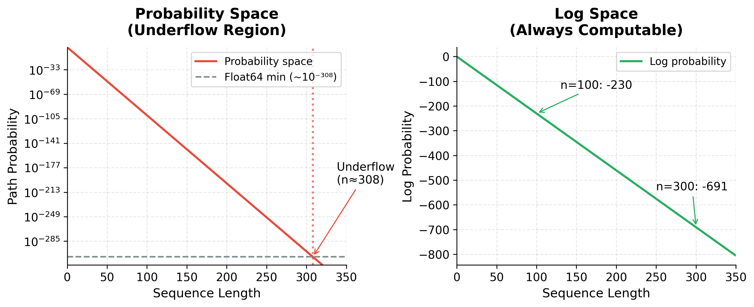
The visualization makes the underflow problem concrete. With a typical per-step probability of 0.1, probability-space values hit the float64 minimum around sequence length 308 and become indistinguishable from zero. Log-space values, in contrast, decrease linearly and remain perfectly representable regardless of sequence length. Even a 1000-word document produces a log probability around -2300, large but entirely computable.
Log-space computation is essential for practical implementations. The algorithm produces identical paths but with stable numerics.
Complexity Analysis
The Viterbi algorithm's efficiency comes from its dynamic programming structure. Let's analyze the time and space requirements.
Time Complexity
For a sequence of length with possible states:
- Initialization: operations to set up the first column
- Recursion: For each of the remaining positions, we compute cells. Each cell considers predecessors. Total:
- Backtracking: to trace back through the path
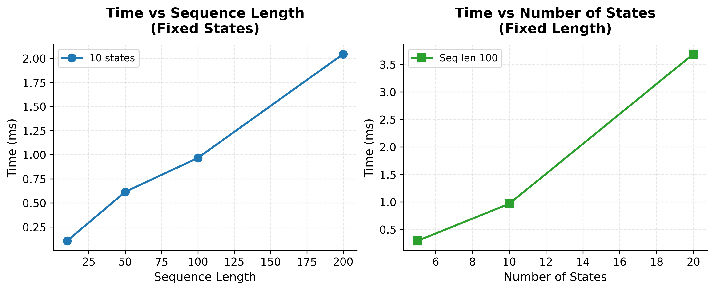
The overall time complexity is , which is linear in sequence length and quadratic in the number of states.
The benchmarks confirm the theoretical complexity. Doubling sequence length roughly doubles runtime (linear scaling), while doubling the number of states roughly quadruples runtime (quadratic scaling). Even with 20 states and 200-word sequences, Viterbi completes in tens of milliseconds, enabling real-time tagging in production systems.
Space Complexity
The algorithm stores:
- Viterbi table: scores
- Backpointers: references
Total space is . However, if we only need the final path and not the full table, we can reduce space to by keeping only two columns at a time, though we'd need to run a second pass to recover the path.
Implementing Viterbi Efficiently
A production implementation incorporates several optimizations beyond the basic algorithm. Let's build a more efficient version.
This implementation uses NumPy's vectorized operations to compute scores for all states simultaneously, avoiding Python loops over states. The key insight is that the inner loop over predecessors becomes a matrix operation.
The NumPy implementation produces the same results as the dictionary-based version but runs significantly faster for large state spaces. The log probability is negative (as expected for log probabilities) and represents the joint probability of the path and observations. The vectorized approach eliminates Python loops over states, leveraging NumPy's optimized C implementations.
Sparse Transitions
Many HMMs have sparse transition matrices where most transitions have zero probability. We can exploit this by only considering valid transitions:
For BIO tagging where I-tags can only follow B-tags or I-tags of the same type, sparse transitions significantly reduce computation. With 9 entity types, you have 19 tags: one O tag plus B and I tags for each entity type (9 × 2 + 1 = 19). A dense transition matrix has entries, but valid transitions are far fewer since I-LOC cannot follow B-PER.
Viterbi for Beam Search Foundation
While Viterbi finds the single best path, many applications need the best paths. Neural sequence models often use beam search, which maintains the top partial hypotheses at each step. Beam search is essentially a pruned version of Viterbi.
Beam search is a heuristic search algorithm that explores the most promising paths in parallel. At each step, it keeps only the top (beam width) partial sequences, pruning less promising alternatives.
The connection to Viterbi is direct: if we set the beam width to equal the number of states, beam search becomes equivalent to Viterbi. Smaller beam widths trade optimality for speed.
The comparison reveals the tradeoff between beam width and optimality. Greedy search (k=1) may find a suboptimal path because it prunes too aggressively. As beam width increases, we retain more hypotheses and are more likely to find the optimal solution. With beam width equal to the number of states, beam search becomes exact Viterbi. In practice, small beam widths (3-10) often find near-optimal solutions while running much faster than exact Viterbi.
Beam search with is greedy decoding. As increases, we approach Viterbi's optimal solution. The tradeoff is computation time: beam search is where is the beam width, compared to Viterbi's .
Constrained Decoding
In sequence labeling, certain tag transitions are invalid. An I-LOC tag cannot follow a B-PER tag. Rather than learning these constraints from data, we can enforce them during decoding by setting invalid transition probabilities to zero (or negative infinity in log space).
The constraints follow BIO semantics: I-tags can only continue entities of the same type, while B-tags and O can follow any tag. Invalid transitions like O → I-PER (starting an entity with a continuation tag) or B-PER → I-LOC (continuing a PER entity as LOC) are explicitly forbidden. By setting these transition probabilities to negative infinity during Viterbi decoding, we guarantee the output is always a well-formed BIO sequence.
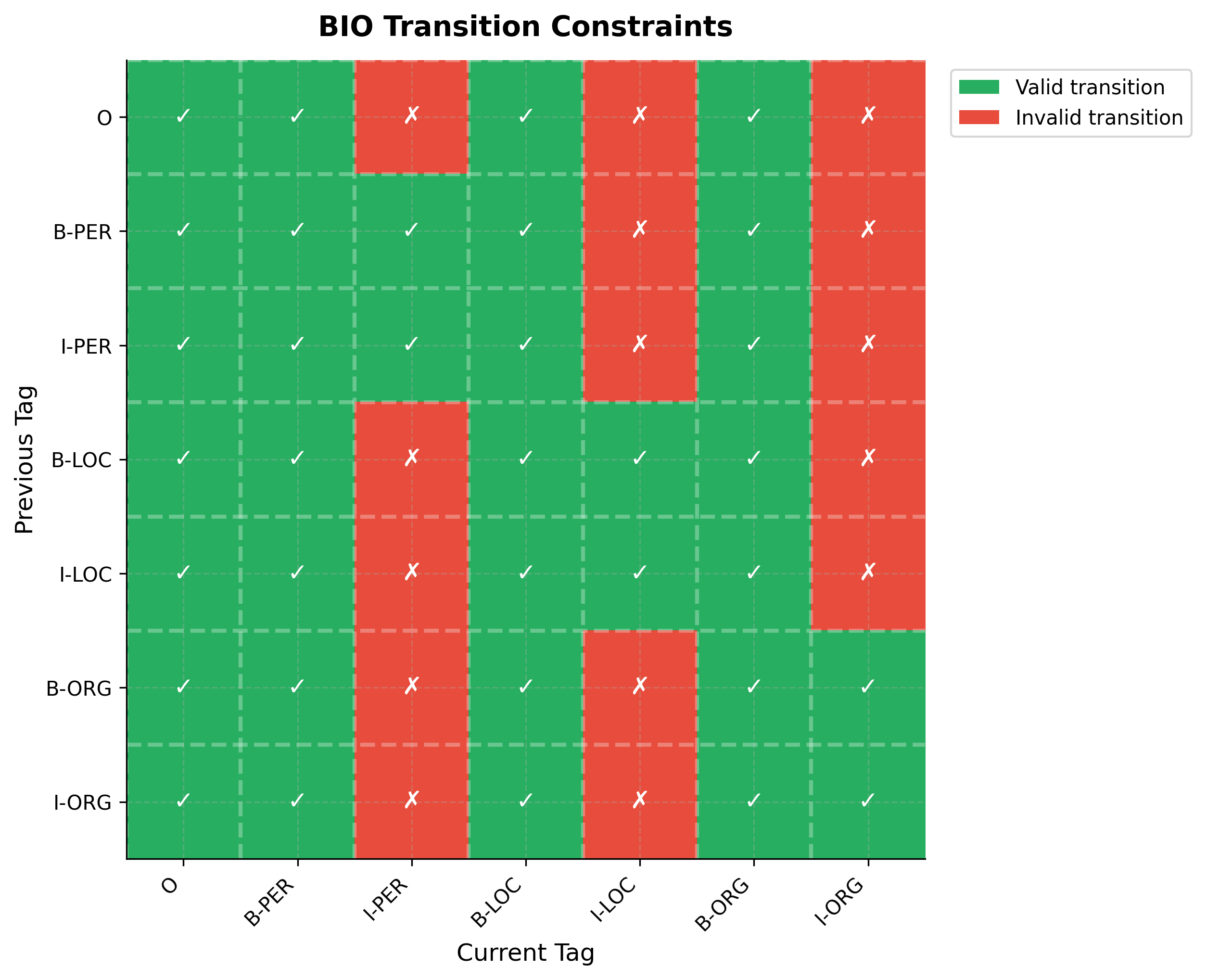
The heatmap reveals the structure of BIO constraints at a glance. The first row and column (O tag) show that O can follow anything and anything can precede O. The B-tags (columns 2, 4, 6) are fully green because they can follow any tag since they start new entities. The distinctive pattern appears in the I-tag columns: each I-tag has exactly two green cells, corresponding to its matching B and I tags. This sparsity (25 valid out of 49 possible transitions) enables significant optimization during Viterbi decoding.
Constrained decoding ensures the output is always a valid BIO sequence, even if the model's raw scores would suggest otherwise. This is particularly important for neural models that don't explicitly model transition constraints.
Limitations and Practical Considerations
The Viterbi algorithm is optimal for first-order Markov models where the current state depends only on the previous state. Several limitations arise in practice:
-
Higher-order dependencies exist in natural language. The optimal tag for a word might depend on tags two or three positions back. Extending Viterbi to second-order Markov models is possible but increases complexity to since we must track pairs of previous states.
-
Non-local features are common in neural sequence models. A BiLSTM encodes the entire sentence before making predictions, so the score at each position depends on the full context, not just the previous tag. CRF layers on top of neural models use Viterbi for decoding, but the emission scores come from the neural network rather than simple probability tables.
-
Approximate inference becomes necessary with large state spaces. In machine translation, the "states" are partial translations with exponentially many possibilities. Beam search provides a practical approximation, trading optimality for tractability.
-
Label dependencies beyond transitions sometimes matter. In some tagging schemes, the entity type of a word might depend on entity types earlier in the sentence, not just the immediately preceding tag. Such long-range dependencies require more sophisticated inference methods.
Despite these limitations, Viterbi remains the workhorse algorithm for sequence labeling. Its efficiency, optimality guarantees for Markov models, and straightforward implementation make it the right choice for most POS tagging and NER systems. When combined with neural feature extractors and CRF output layers, it achieves state-of-the-art results on many benchmarks.
Summary
The Viterbi algorithm solves the optimal path problem for sequence labeling. Given a sequence of observations and a model with transition and emission probabilities, it finds the single best sequence of hidden states in time linear in sequence length.
The key ideas covered in this chapter:
Dynamic programming makes the exponential search space tractable. By storing the best score for each state at each position, we avoid recomputing shared subsequences. The complexity enables real-time tagging of long documents.
Backpointer tracking enables path reconstruction. At each cell in the Viterbi table, we record which predecessor achieved the maximum score. After filling the table, we trace back from the best final state to recover the optimal path.
Log-space computation prevents numerical underflow. Working with log probabilities converts products to sums, keeping values in a representable range even for long sequences. This is essential for any practical implementation.
Constrained decoding enforces structural requirements. For BIO tagging, we set invalid transition probabilities to zero, ensuring the output is always a valid tag sequence regardless of what the model's raw scores suggest.
Beam search connects to Viterbi as an approximation. By keeping only the top hypotheses at each step, beam search trades optimality for speed. With beam width equal to the number of states, it recovers Viterbi exactly.
Key Parameters and Functions
When implementing or using Viterbi decoding, these parameters control behavior:
- states: The set of possible hidden states (tags). Larger state sets increase computation quadratically
- transition_prob: Matrix or dictionary of values. Sparse matrices enable optimization
- emission_prob: Matrix or dictionary of values. In neural models, these come from network outputs
- start_prob: Initial state distribution . Often uniform or learned from data
- beam_width: For approximate decoding, controls the number of hypotheses retained. Larger values approach exact Viterbi
The next chapter introduces Conditional Random Fields, which generalize HMMs by allowing arbitrary feature functions while still using Viterbi for efficient decoding.
Quiz
Ready to test your understanding? Take this quick quiz to reinforce what you've learned about the Viterbi algorithm and optimal sequence decoding.

Comments