

Master neural network activation functions including sigmoid, tanh, ReLU variants, GELU, Swish, and Mish. Learn when to use each and why.

This article is part of the free-to-read Language AI Handbook
Choose your expertise level to adjust how many terms are explained. Beginners see more tooltips, experts see fewer to maintain reading flow. Hover over underlined terms for instant definitions.
Activation Functions
Neural networks derive their power from non-linearity. Without activation functions, even the deepest network would collapse into a simple linear transformation, no matter how many layers you stack. Activation functions are the secret ingredient that allows neural networks to learn complex, non-linear patterns in data.
In this chapter, we explore the evolution of activation functions, from the biologically-inspired sigmoid to modern innovations like GELU and Swish. You will understand not just what each function computes, but why it was designed that way and when to use it.
Why Non-Linearity Matters
Consider stacking two linear transformations. If the first layer computes and the second computes , we can substitute and simplify:
where:
- : the input vector
- : weight matrices for layers 1 and 2
- : bias vectors for layers 1 and 2
- : the hidden representation after the first layer
- : the final output
The result is equivalent to a single linear layer with weight matrix and bias . No matter how many layers we add, without non-linearity, the network can only learn linear decision boundaries.
Activation functions break this limitation. By applying a non-linear function after each linear transformation, we enable networks to approximate arbitrarily complex functions.
The Sigmoid Function
The sigmoid function was one of the first activation functions used in neural networks. Its S-shaped curve smoothly maps any real number to a value between 0 and 1, making it interpretable as a probability.
Mathematical Definition
The sigmoid function is defined as:
where:
- : the input value (pre-activation), which can be any real number
- : Euler's number (approximately 2.718)
- : the output, constrained to the range
The function works by exponentiating the negative input. When is large and positive, approaches 0, so . When is large and negative, becomes very large, pushing toward 0. At , we get .
The Derivative
The sigmoid has an elegant derivative that can be expressed in terms of itself:
where:
- : the derivative of sigmoid with respect to
- : the sigmoid function evaluated at
This property makes gradient computation efficient. Once we compute the forward pass value , we can immediately compute the gradient without re-evaluating the exponential.
The Saturation Problem
The maximum value of the derivative occurs at , where . This means the gradient is at most 0.25, and it rapidly approaches 0 as increases. This phenomenon is called saturation.
When inputs to sigmoid neurons are very large or very small, the gradient becomes negligibly small. During backpropagation, these tiny gradients multiply together across layers, causing gradients to "vanish" in deep networks. This makes training deep networks with sigmoid activations extremely difficult.
Let's visualize the sigmoid function and its derivative to understand saturation:
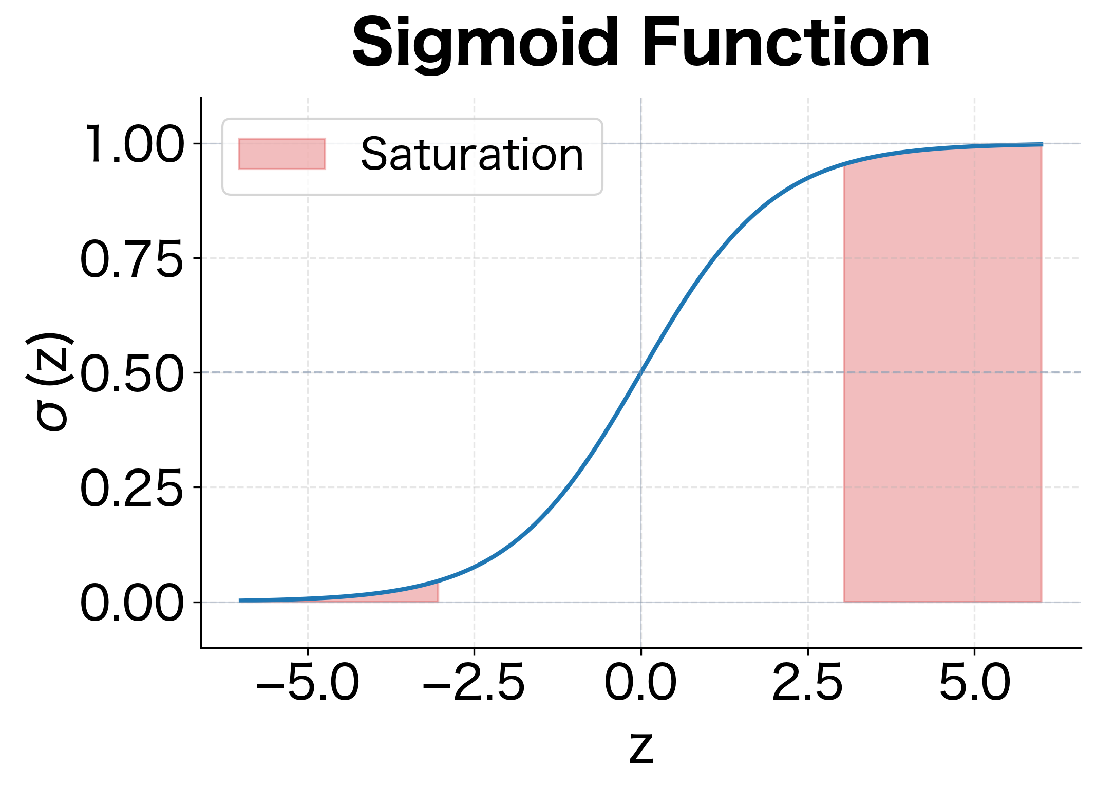
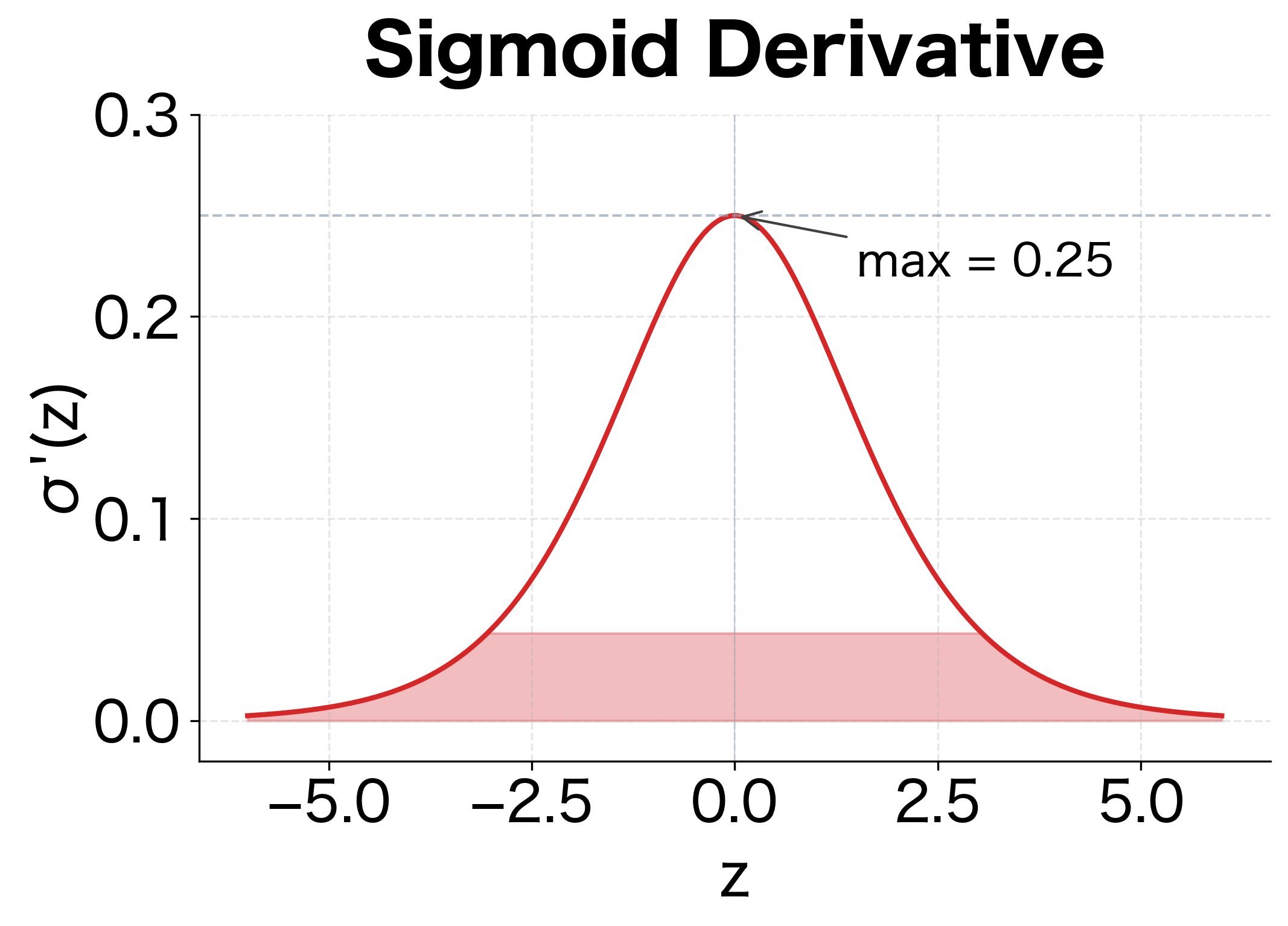
The shaded regions highlight where saturation occurs. In these zones, the gradient is nearly zero, making learning extremely slow or impossible.
The Hyperbolic Tangent (tanh)
The hyperbolic tangent function addresses one limitation of sigmoid: it is zero-centered, meaning its outputs are symmetric around zero. This property helps with gradient flow during training.
Mathematical Definition
where:
- : the input value
- : exponentials of the positive and negative input
- : the output, constrained to the range
An equivalent formulation relates tanh to sigmoid:
This shows that tanh is essentially a rescaled and shifted version of sigmoid, mapping to instead of .
The Derivative
where:
- : the derivative of tanh with respect to
- : the square of the tanh output
At , the derivative equals 1, which is four times larger than sigmoid's maximum gradient of 0.25. This stronger gradient signal helps mitigate, though not eliminate, the vanishing gradient problem.
Comparing Sigmoid and Tanh
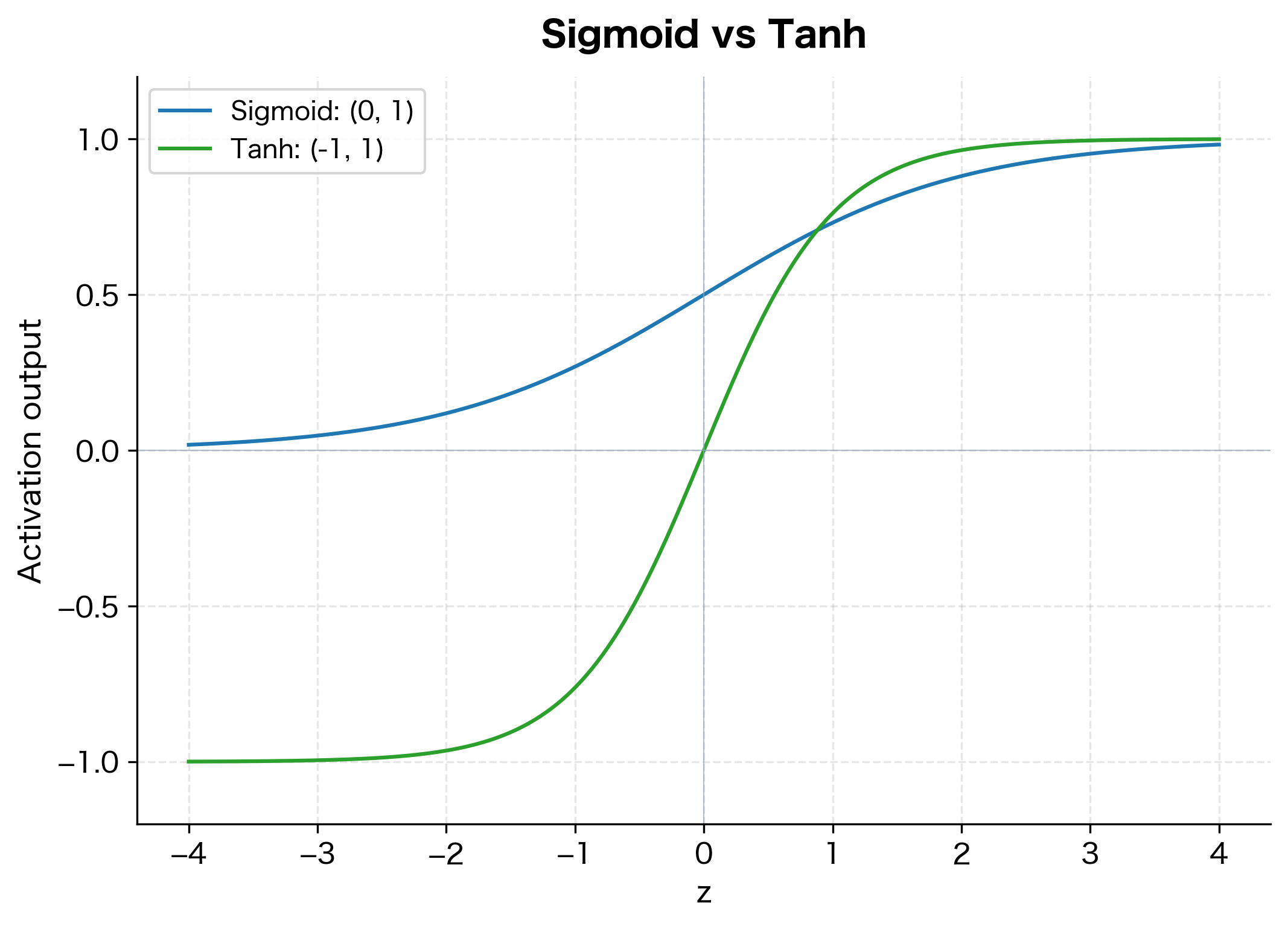
Both sigmoid and tanh suffer from saturation for large values. However, tanh's zero-centered output makes it preferable for hidden layers, while sigmoid remains useful for output layers when you need probabilities.
Rectified Linear Unit (ReLU)
ReLU revolutionized deep learning. Its simplicity, computational efficiency, and resistance to vanishing gradients made training deep networks practical for the first time.
Mathematical Definition
where:
- : the input value
- : returns if positive, otherwise 0
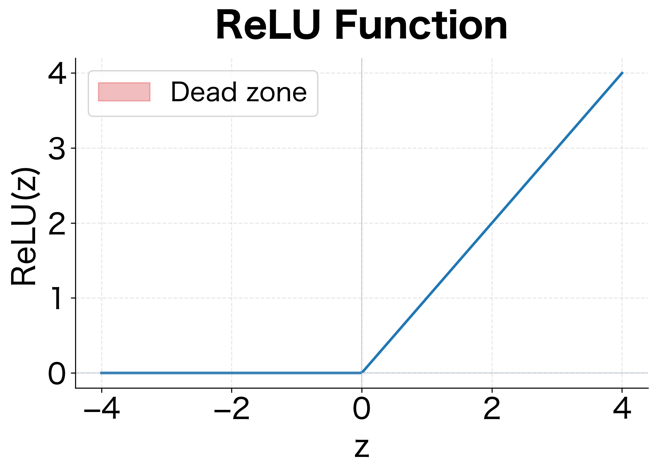
The function is piecewise linear: it passes positive values unchanged and clips negative values to zero.
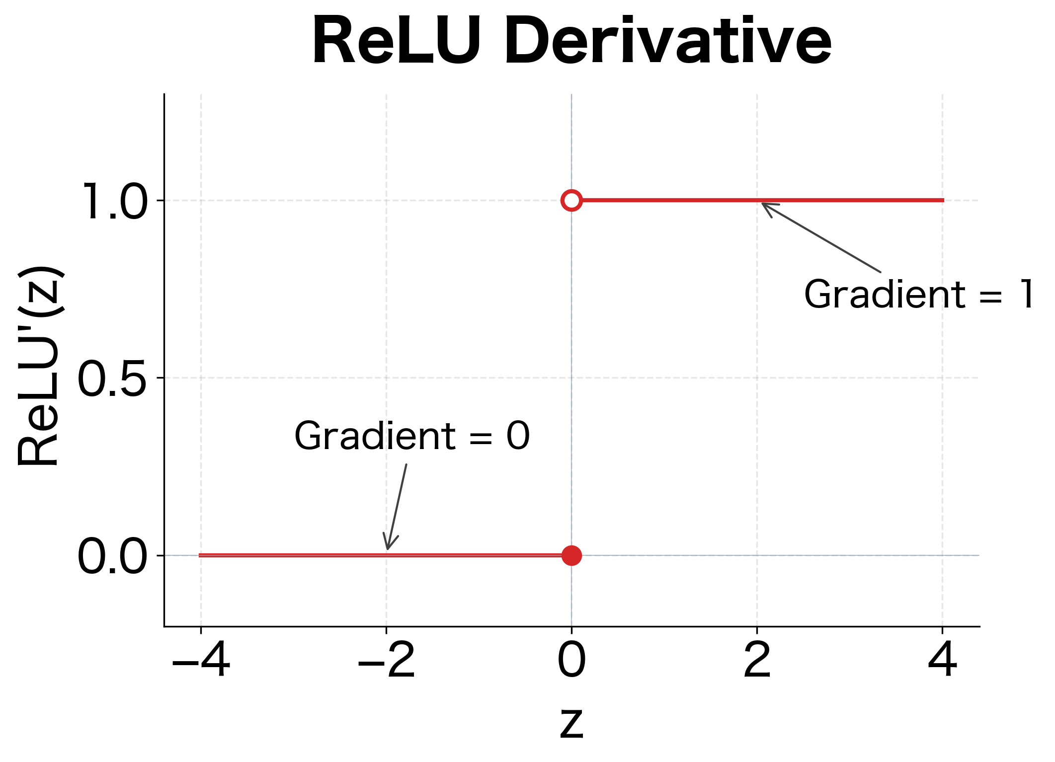
The Derivative
At exactly , the derivative is technically undefined, but in practice, we typically set it to 0 or 1.
The key insight is that for positive inputs, the gradient is exactly 1. This means gradients flow through ReLU layers without diminishing, solving the vanishing gradient problem that plagued sigmoid and tanh.
The Dying ReLU Problem
While ReLU solves vanishing gradients, it introduces a new issue: neurons can "die" during training.
If a ReLU neuron's weights are updated such that its pre-activation becomes negative for all training examples, the neuron outputs zero for every input. Since the gradient is also zero for negative inputs, the neuron can never recover. It becomes permanently inactive, effectively reducing the network's capacity.
This typically happens when:
- The learning rate is too high, causing large weight updates
- Poor weight initialization pushes many neurons into negative territory
- Strong negative gradients shift the bias terms too far negative
Leaky ReLU and Parametric ReLU
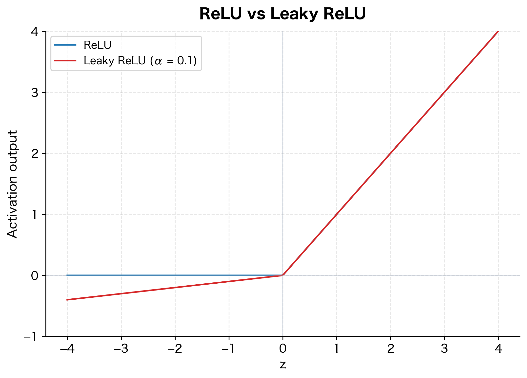
Leaky ReLU addresses the dying ReLU problem by allowing a small, non-zero gradient when the input is negative.
Mathematical Definition
where:
- : the input value
- : a small positive constant, typically 0.01
- : the scaled negative input, giving a small but non-zero output
The function can also be written compactly as:
Parametric ReLU (PReLU)
PReLU takes this further by making a learnable parameter:
The key difference is that is learned during training via backpropagation, allowing the network to determine the optimal slope for negative inputs.
Derivative
For both Leaky ReLU and PReLU:
The small but non-zero gradient for negative inputs allows the neuron to continue learning even when it receives negative pre-activations.
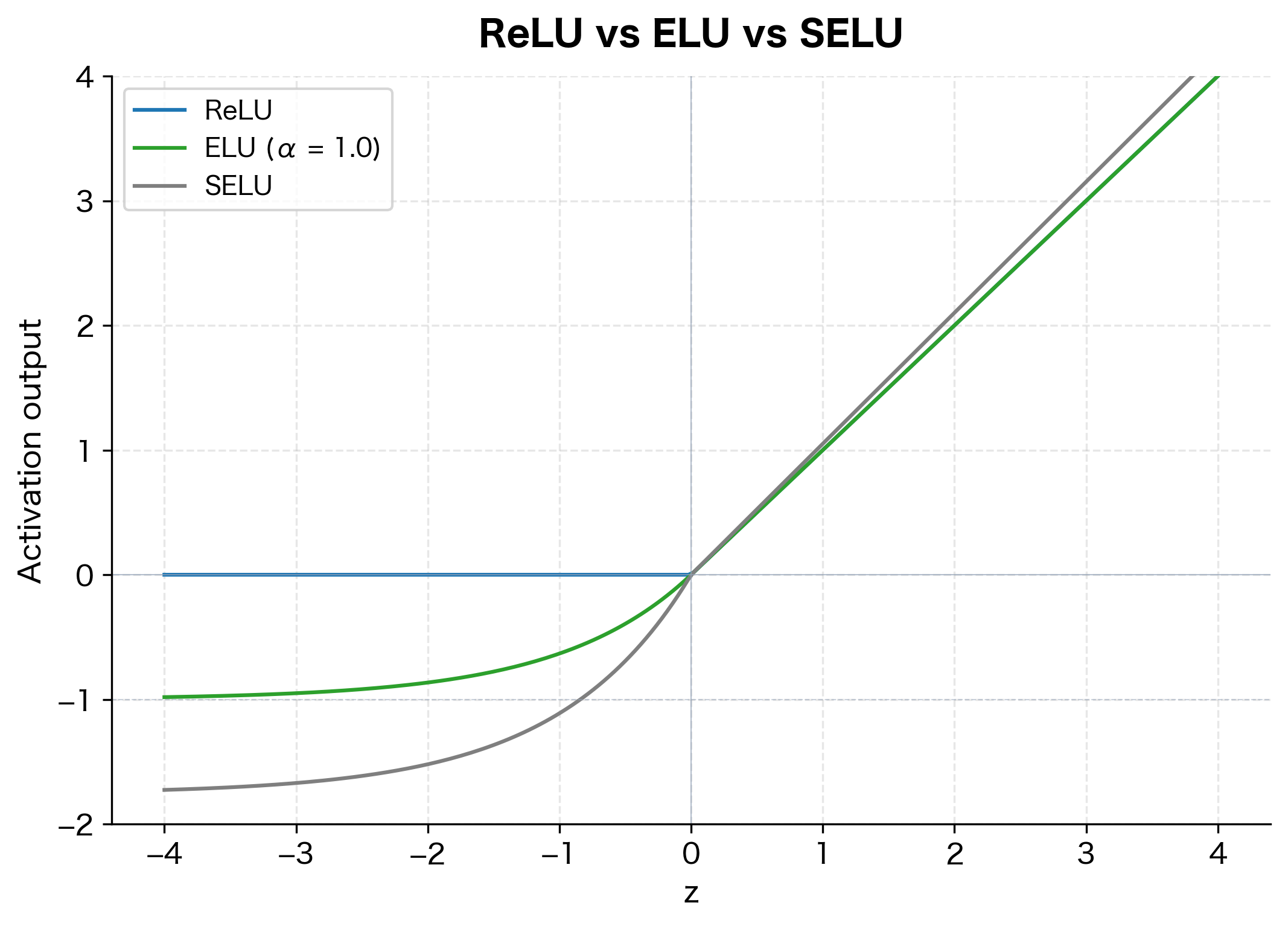
Exponential Linear Unit (ELU)
ELU provides smooth, differentiable transitions at zero and pushes mean activations closer to zero, which can accelerate learning.
Mathematical Definition
where:
- : the input value
- : a hyperparameter controlling the saturation value for negative inputs (typically 1.0)
- : an exponential term that approaches as
For large negative inputs, ELU saturates at . This saturation provides noise robustness by limiting the influence of large negative values.
The Derivative
Note that for , the derivative can be computed from the function value itself, similar to sigmoid's self-referential gradient.
Scaled Exponential Linear Unit (SELU)
SELU is a self-normalizing variant of ELU. When used with proper weight initialization, SELU activations automatically converge to zero mean and unit variance, eliminating the need for batch normalization.
where the specific values are:
These constants were derived analytically to ensure self-normalizing properties.
Gaussian Error Linear Unit (GELU)
GELU has become the default activation function in transformer architectures like BERT and GPT. Unlike ReLU, which deterministically zeroes out negative values, GELU applies a smooth, probabilistic gating.
Intuition
GELU can be understood through a stochastic regularization lens. Imagine each neuron is randomly multiplied by either 0 or 1, where the probability of being "on" depends on how positive the input is. GELU computes the expected value of this stochastic process:
where is a standard normal random variable.
Mathematical Definition
The formal definition uses the cumulative distribution function (CDF) of the standard normal distribution:
where:
- : the input value
- : the CDF of the standard normal distribution, i.e.,
- : the input scaled by the probability that a standard normal is less than
The CDF is defined as:
where is the error function.
Practical Approximation
Computing the error function can be expensive. A commonly used approximation is:
This approximation is accurate to within a few percent and is computationally efficient.
The Derivative
The derivative of GELU involves both the CDF and the probability density function (PDF) of the standard normal:
where:
- : the standard normal CDF
- : the standard normal PDF
This derivative is always positive for large positive , and smoothly transitions through zero.
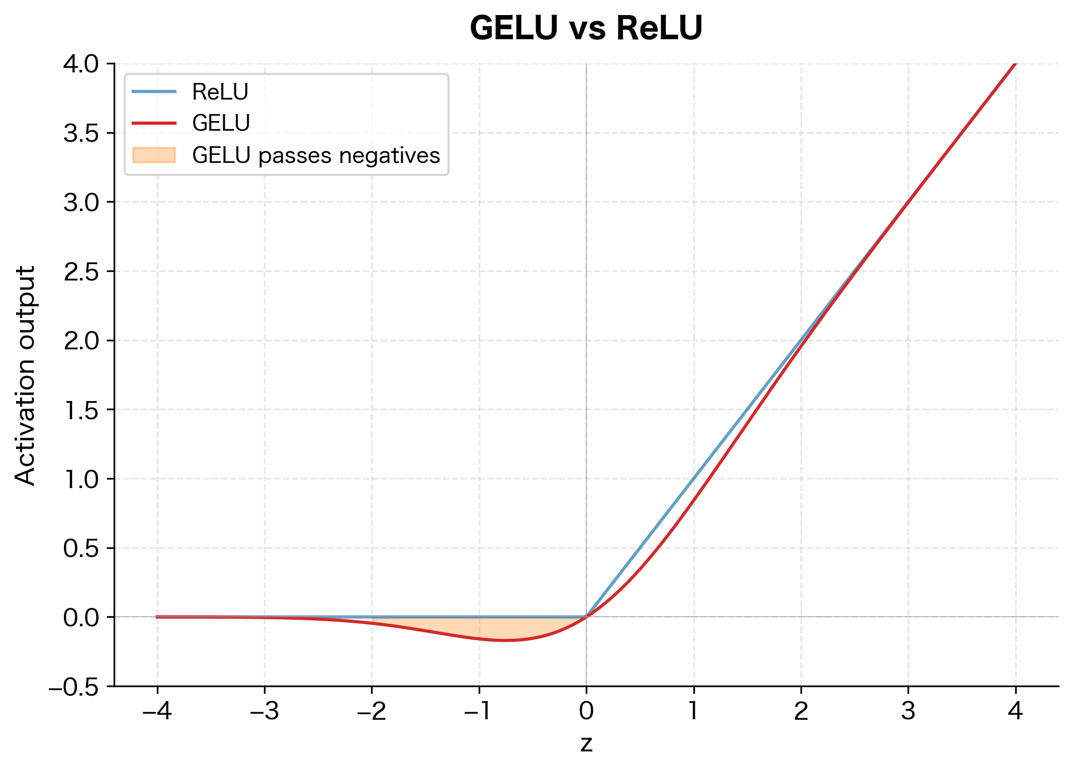
The key difference is visible near zero: GELU smoothly curves through the origin, allowing small negative values to pass through with reduced magnitude. This smooth gating is believed to help with gradient flow and model expressiveness.
Swish and Mish
Swish and Mish are modern activation functions discovered through automated search and designed to combine the benefits of ReLU-like behavior with smooth gradients.
Swish
Swish was discovered by Google researchers using automated search techniques:
where:
- : the input value
- : the sigmoid function
- : a learnable or fixed parameter (often )
- : the input scaled by the sigmoid of itself
When , this simplifies to:
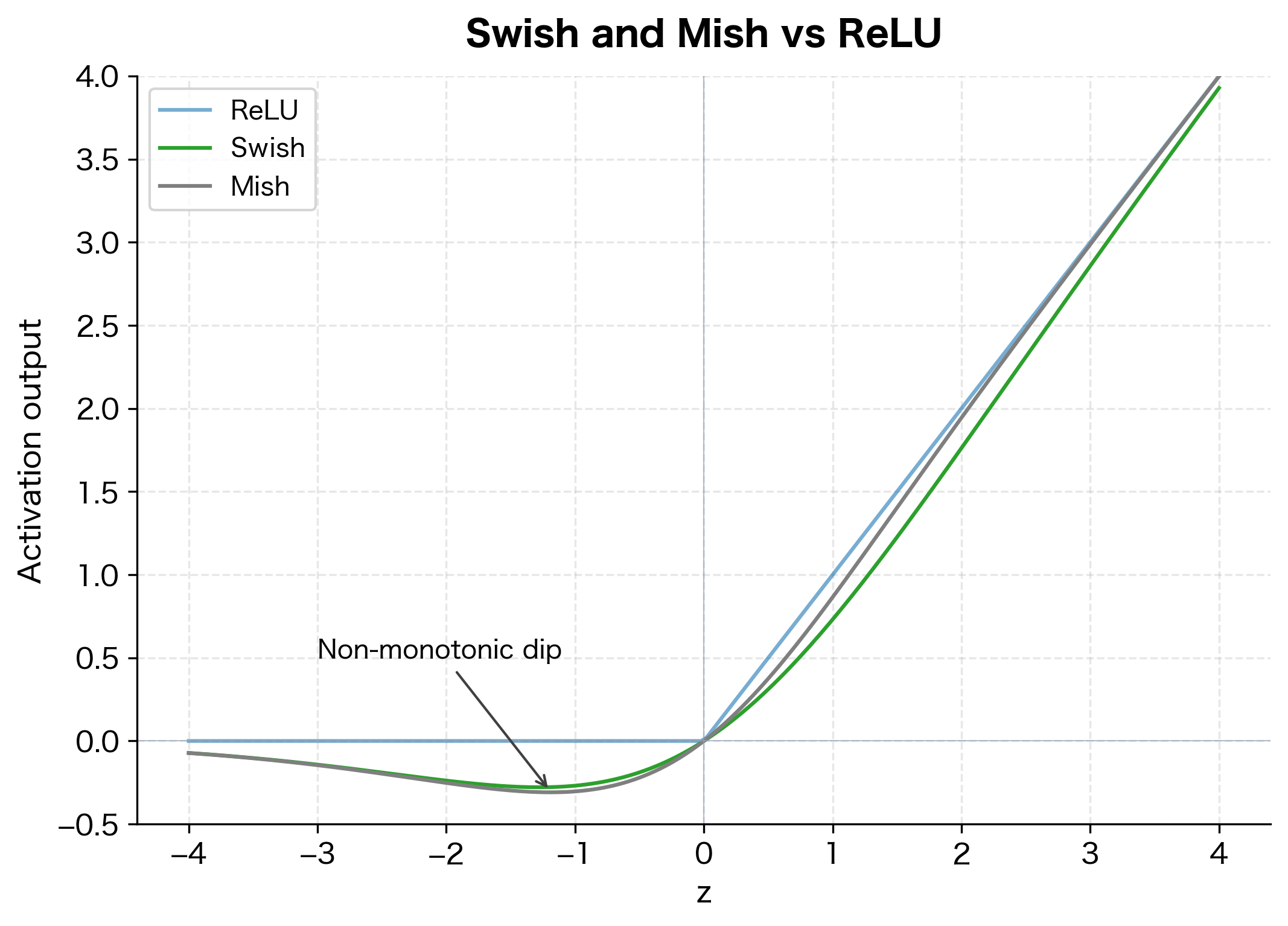
Swish is non-monotonic: it dips below zero for negative inputs before rising again. This allows small negative gradients to flow backward, potentially helping escape local minima.
Mish
Mish uses the softplus function and tanh for an even smoother curve:
where:
- : a smooth approximation to ReLU
- : the hyperbolic tangent function
Mish has continuous derivatives of all orders, making it particularly smooth. Like Swish, it is non-monotonic with a small negative region.
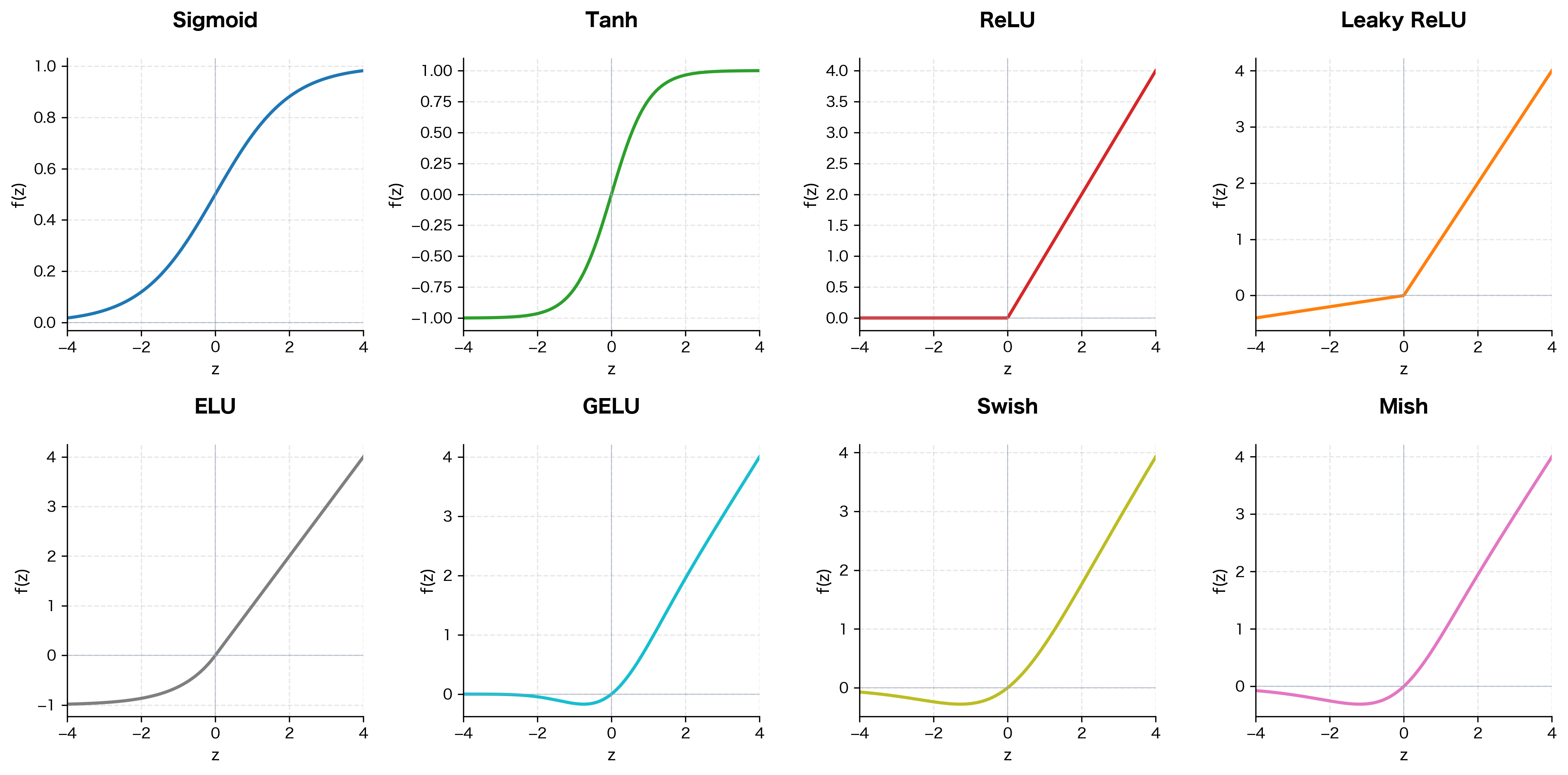
Comparing All Activation Functions
Let's visualize all the activation functions we've covered in a single comprehensive comparison. This 2×4 grid allows direct comparison of each function's behavior, particularly around zero where their differences are most apparent.
Implementation in PyTorch
Let's implement and visualize these activation functions using PyTorch. Modern deep learning frameworks provide optimized implementations of all common activations.
The output shows each activation's behavior at three key points: a negative value, zero, and a positive value. Notice how ReLU completely zeros out negative inputs, while Leaky ReLU preserves a scaled version. GELU and Swish (SiLU) show smooth, non-zero responses even for negative inputs.
Custom Activation Implementation
You can also implement custom activations as simple functions:
The tanh approximation closely matches the exact GELU computation while being computationally efficient. The small differences are negligible in practice.
Choosing Activation Functions
Selecting the right activation function depends on your architecture, task, and computational constraints. Here is a practical guide based on current best practices.
For Hidden Layers in Feedforward Networks
| Activation | Best Use Case | Considerations |
|---|---|---|
| ReLU | Default choice for most networks | Fast, effective, but watch for dying neurons |
| Leaky ReLU | When dying ReLU is a concern | Small computational overhead |
| ELU | When faster convergence is needed | More expensive than ReLU |
| SELU | Self-normalizing networks | Requires specific initialization |
For Transformer Architectures
GELU has become the de facto standard for transformers. Its smooth gating properties align well with the attention mechanism's probabilistic nature. Major models like BERT, GPT, and their variants all use GELU.
For Output Layers
| Task | Activation | Output Range |
|---|---|---|
| Binary classification | Sigmoid | (0, 1) |
| Multi-class classification | Softmax | (0, 1) per class, sum = 1 |
| Regression | None (linear) | Unbounded |
| Bounded regression | Sigmoid or Tanh | Scaled to target range |
For Recurrent Networks (RNNs, LSTMs)
Tanh remains common for recurrent connections because:
- Zero-centered outputs help maintain stable hidden states
- The bounded range prevents activations from exploding
- Gate mechanisms (in LSTMs/GRUs) specifically rely on sigmoid's (0, 1) output
Practical Considerations
When implementing activation functions in production, consider these factors:
Computational Cost: ReLU is the fastest, requiring only a comparison and conditional. Exponential-based functions (sigmoid, tanh, ELU, SELU) are more expensive. GELU requires either the expensive error function or a polynomial approximation.
Numerical Stability: Sigmoid and softmax can overflow for very large inputs. Use numerically stable implementations that subtract the maximum value before exponentiating.
Initialization Compatibility: Some activations work best with specific initialization schemes. He initialization pairs well with ReLU variants, while Xavier/Glorot initialization suits tanh and sigmoid.
Gradient Flow: For very deep networks, favor activations with gradients that neither vanish nor explode. ReLU and its variants generally provide good gradient flow, while sigmoid and tanh can cause vanishing gradients.
Summary
Activation functions are the non-linear transformations that give neural networks their expressive power. The field has evolved from biologically-inspired functions like sigmoid to modern innovations designed for specific architectural needs.
Key takeaways:
-
Sigmoid and tanh were early standards but suffer from vanishing gradients in deep networks. Sigmoid remains useful for output layers when probabilities are needed.
-
ReLU revolutionized deep learning with its simple, sparse, and gradient-preserving properties. The dying ReLU problem led to variants like Leaky ReLU and ELU.
-
GELU provides smooth, probabilistic gating and has become the standard for transformer architectures. Its stochastic interpretation aligns well with the attention mechanism.
-
Swish and Mish offer smooth, non-monotonic alternatives that can outperform ReLU on certain tasks while maintaining good gradient flow.
-
For practical applications: Start with ReLU for general feedforward networks, GELU for transformers, and task-appropriate functions for output layers.
The choice of activation function can significantly impact training dynamics and final performance. While the differences may seem subtle, they compound across millions of neurons and billions of parameters in modern networks.
Quiz
Ready to test your understanding? Take this quick quiz to reinforce what you've learned about activation functions in neural networks.

Comments