Gradient Clipping: Preventing Exploding Gradients in Deep Learning

Deep neural networks are powerful function approximators, but training them can be surprisingly fragile. One moment your loss is decreasing steadily, the next it explodes to infinity. The culprit? Exploding gradients. When gradients grow too large during backpropagation, weight updates become catastrophically destabilizing, and training collapses.

Gradient clipping provides a simple but effective solution. By capping gradients at a maximum threshold before applying updates, we prevent the runaway feedback loops that cause explosions. This technique is essential for training recurrent neural networks, transformers, and many other deep architectures. Without it, models with long computational paths would be nearly impossible to train.

This chapter covers how to detect exploding gradients, the two main clipping strategies (by value and by global norm), and when to apply each approach. We'll implement gradient clipping from scratch and explore how to choose appropriate thresholds through gradient norm monitoring.

During backpropagation, gradients flow backward through the network, accumulating contributions from each layer. In deep networks or recurrent architectures, this can create a feedback loop where gradients compound multiplicatively.

Consider a simple recurrent network processing a sequence of $T$ timesteps. At each step, the gradient is multiplied by the weight matrix $\mathbf{W}$. If the largest eigenvalue of that matrix exceeds 1, gradients grow exponentially. After $T$ multiplications, the gradient magnitude scales as:

where:

• $\|\mathbf{g}_0\|$: the initial gradient magnitude at the output layer
• $\|\mathbf{g}_T\|$: the gradient magnitude after backpropagating through $T$ timesteps
• $\lambda_{\max}$: the largest eigenvalue of the weight matrix (or its spectral norm)
• $T$: the number of timesteps (or layers) the gradient passes through

With $T = 100$ timesteps and $\lambda_{\max} = 1.1$, the gradient grows by a factor of $1.1^{100} \approx 13,781$. Even this modest 10% amplification per step compounds into a catastrophic explosion.

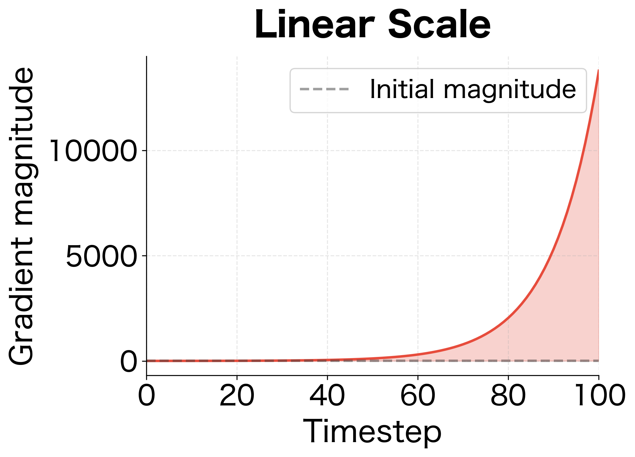
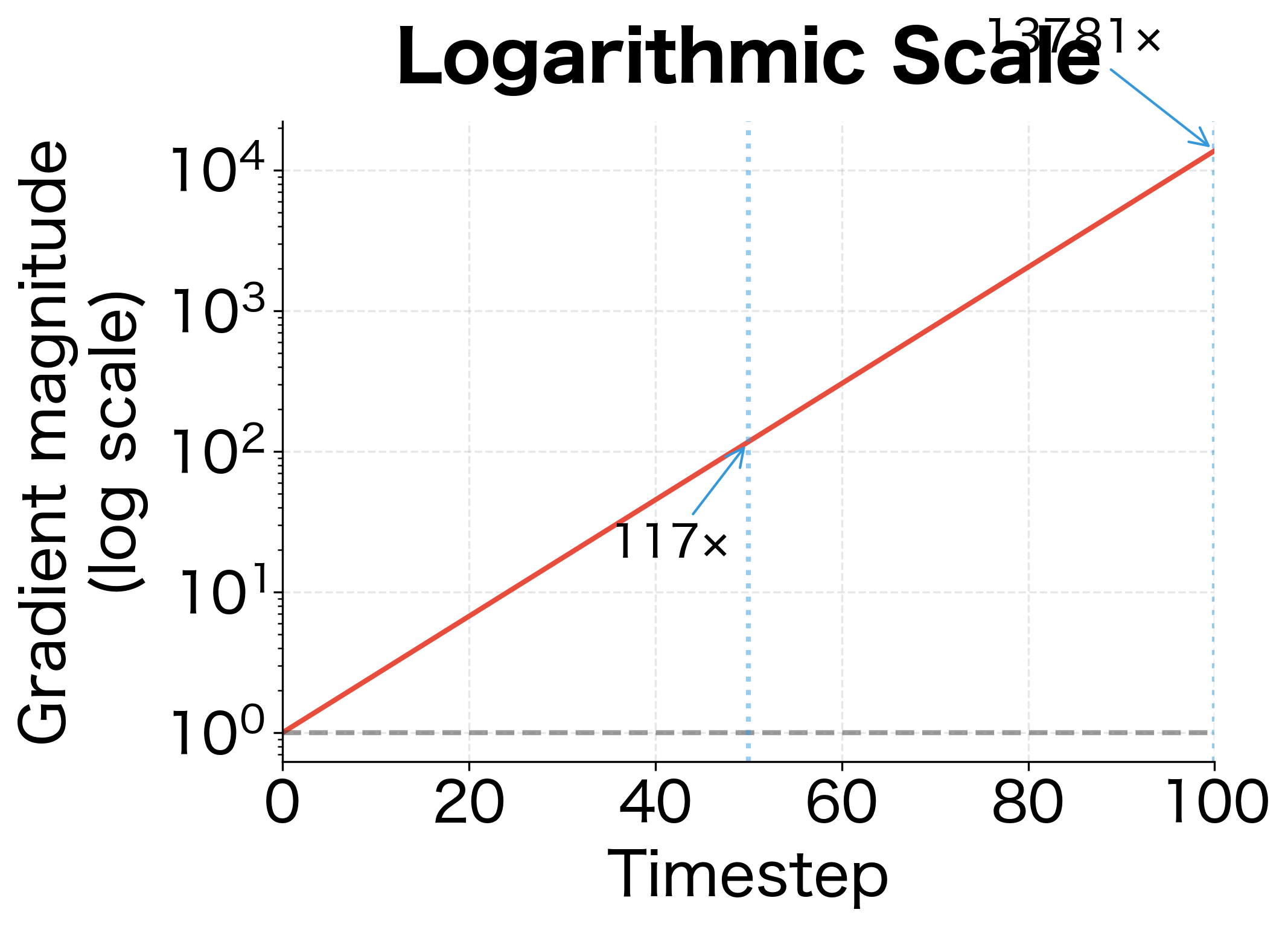
The exponential growth is striking. With just a 10% amplification per step, the gradient grows nearly 14,000 times larger by the end of the sequence. This illustrates why even seemingly small spectral norms above 1.0 become catastrophic in deep or recurrent networks. In practice, these explosive gradients lead to NaN losses, parameter values shooting to infinity, and complete training failure.

Before clipping, you need to know when gradients are problematic. The clearest signal is the gradient norm, which measures the overall magnitude of gradients across all parameters. For a model with parameters $\theta_1, \theta_2, \ldots, \theta_n$, each with gradient $\nabla_{\theta_i} L$, the global L2 norm is:

where:

• $\nabla_{\theta_i} L$: the gradient of the loss $L$ with respect to parameter $\theta_i$ (a tensor)
• $\|\nabla_{\theta_i} L\|_2$: the L2 norm of that parameter's gradient
• $\|\nabla L\|_2$: the global gradient norm across all parameters

This single scalar summarizes the entire gradient's magnitude, making it easy to monitor and compare across training steps.

The global gradient norm for this network is relatively modest, typical for a well-initialized shallow network on random data. The per-layer breakdown shows how each parameter contributes to the total. In practice, you'd monitor this norm over training batches to detect sudden spikes, which signal potential gradient explosions.

Several architectural and training choices make gradient explosions more likely:

• Deep architectures: More layers mean more gradient multiplications. Each layer's Jacobian contributes to the product, and if many have spectral norms greater than 1, gradients explode.
• Recurrent networks: RNNs and LSTMs process sequences by repeatedly applying the same weights. Long sequences create deep computational graphs with shared parameters.
• Large learning rates: Even moderate gradients become destructive updates with high learning rates. The explosion may be in the update magnitude rather than the gradient itself.
• Improper initialization: Weight initialization that starts parameters too large can push networks into explosive regimes from the first forward pass.

Now that we understand why exploding gradients are dangerous, let's examine how to prevent them. The core idea is simple: if gradients become too large, we shrink them before applying the weight update. But "too large" can mean different things, and how we shrink gradients matters for optimization. This leads to two distinct strategies, each with its own geometric interpretation and trade-offs.

When we say a gradient is "too large," we could mean two different things:

1. Individual elements are extreme: Some specific gradient values are huge, even if others are small
2. The overall magnitude is extreme: The gradient vector as a whole points too far, even if no single element is unusual

These two interpretations lead to fundamentally different clipping strategies. The first gives us "clip by value," which treats each gradient element independently. The second gives us "clip by global norm," which treats the gradient as a unified vector and scales it uniformly. Understanding this distinction is crucial, because the choice affects not just the magnitude of updates but potentially their direction.

The simplest approach treats each gradient element as an independent quantity to be bounded. If any element exceeds a threshold $\tau$, we clamp it to that threshold. Elements within bounds remain unchanged.

Think of this geometrically: we're constraining the gradient to lie within a hypercube centered at the origin. In 2D, this is a square; in 3D, a cube; in higher dimensions, a hypercube with sides of length $2\tau$.

Let's see this in action with a concrete example. We'll create a gradient vector with some moderate values and some extreme outliers, then apply clip by value.

Three of the six elements exceeded the threshold and were clamped. The extreme values at indices 0, 4, and 5 are now bounded to ±2.0, while the moderate values at indices 1, 2, and 3 pass through unchanged.

This asymmetric treatment reveals the core limitation of clip by value: it changes the gradient direction. Before clipping, the gradient might have pointed predominantly toward adjusting parameter 4 (with gradient 10.0). After clipping, that dimension is capped at 2.0, the same as dimension 3. The relative importance of different parameters has been distorted. In optimization terms, we're no longer moving in the direction the loss landscape suggested, but in a direction bent by our clipping constraints.

The direction distortion problem motivates a different approach. Instead of asking "is each element too large?", we ask "is the gradient vector as a whole too long?" If yes, we scale the entire vector down uniformly, preserving all relative proportions.

Geometrically, this constrains the gradient to lie within a hypersphere of radius $\tau$ centered at the origin. In 2D, this is a circle; in 3D, a sphere. Any gradient landing outside this sphere gets projected back onto its surface by scaling, not by truncating individual components.

Why does this preserve direction? Consider a gradient vector $\mathbf{g}$ with norm $\|\mathbf{g}\|_2 = 10$ when our threshold is $\tau = 5$. To bring the norm down to 5, we multiply every component by $\frac{5}{10} = 0.5$. Each component shrinks by the same factor, so the ratios between components remain unchanged. The vector points in exactly the same direction, just with half the length.

The key insight is that uniform scaling preserves the update direction. If the original gradient suggested parameter A should change twice as much as parameter B, that relationship holds after clipping. We simply take a smaller step in the same direction.

Let's implement this and verify that direction is preserved. We'll use two gradient tensors representing different parameters and show that their relative proportions remain unchanged after clipping.

The implementation follows three steps:

1. Compute the global norm by summing squared elements across all gradient tensors, then taking the square root
2. Calculate the scaling factor as $\frac{\tau}{\|\mathbf{g}\|_2}$, which will be less than 1 if clipping is needed
3. Apply uniform scaling to every gradient tensor if the norm exceeds the threshold

The results confirm the theory. The original global norm of 11.18 exceeded our threshold of 5.0, triggering clipping. Both gradient tensors were scaled by the same factor (approximately 0.45), bringing the global norm to exactly 5.0. Most importantly, the ratio between corresponding elements remains identical: 0.5 before and 0.5 after. The gradient direction is perfectly preserved.

This is why norm clipping is generally preferred for optimization. When we clip by norm, we're still moving in the direction the loss landscape suggested, just taking a more cautious step. The relative importance of each parameter's update remains unchanged.

The difference between clip by value and clip by norm becomes crystal clear when we visualize them geometrically. Consider a 2D gradient vector, which we can plot as an arrow in a plane. The two clipping methods impose different constraints on where this arrow can point and how long it can be.

Clip by value constrains the gradient to a square (or hypercube in higher dimensions). The boundary is defined by $|g_1| \leq \tau$ and $|g_2| \leq \tau$ independently. A gradient in the corner of this square, like $(3, 3)$ with threshold $\tau = 2$, gets clipped to $(2, 2)$, which changes its direction subtly. But a gradient like $(4, 1)$ with the same threshold becomes $(2, 1)$, dramatically shifting its angle.

Clip by norm constrains the gradient to a circle (or hypersphere). The boundary is defined by $\sqrt{g_1^2 + g_2^2} \leq \tau$. Any gradient outside this circle gets scaled toward the origin until it touches the circle's edge, preserving its angle perfectly.

Let's see both methods applied to the same gradient vector:

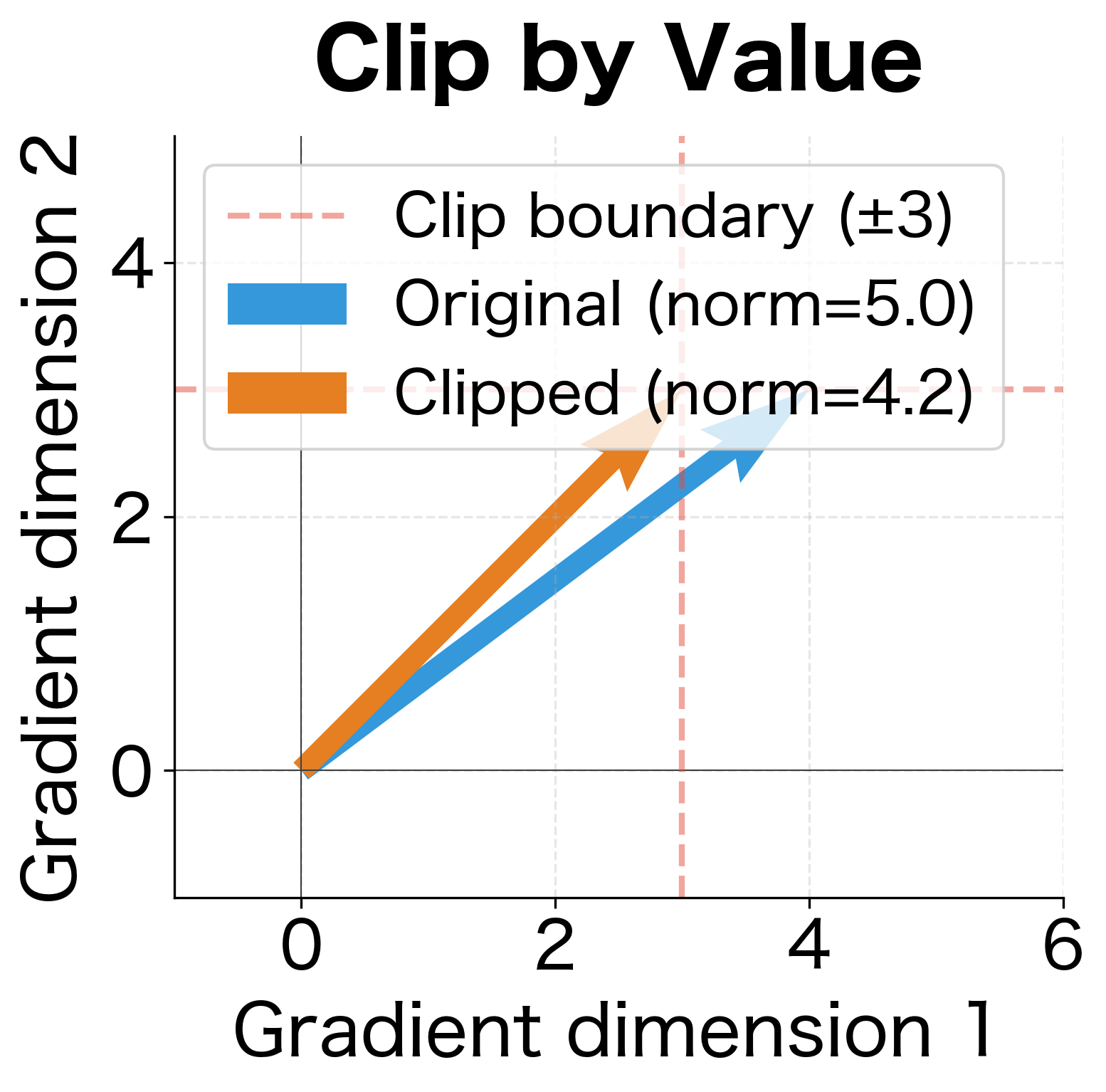
The visualization crystallizes the key insight. On the left, clip by value creates a box (square) constraint. The original gradient $(4, 3)$ lies outside this box, so its first component is clipped to 3. But the second component was already within bounds and remains unchanged. The result? The clipped vector points at a different angle than the original, pulling the update direction away from where the loss landscape suggested we should go.

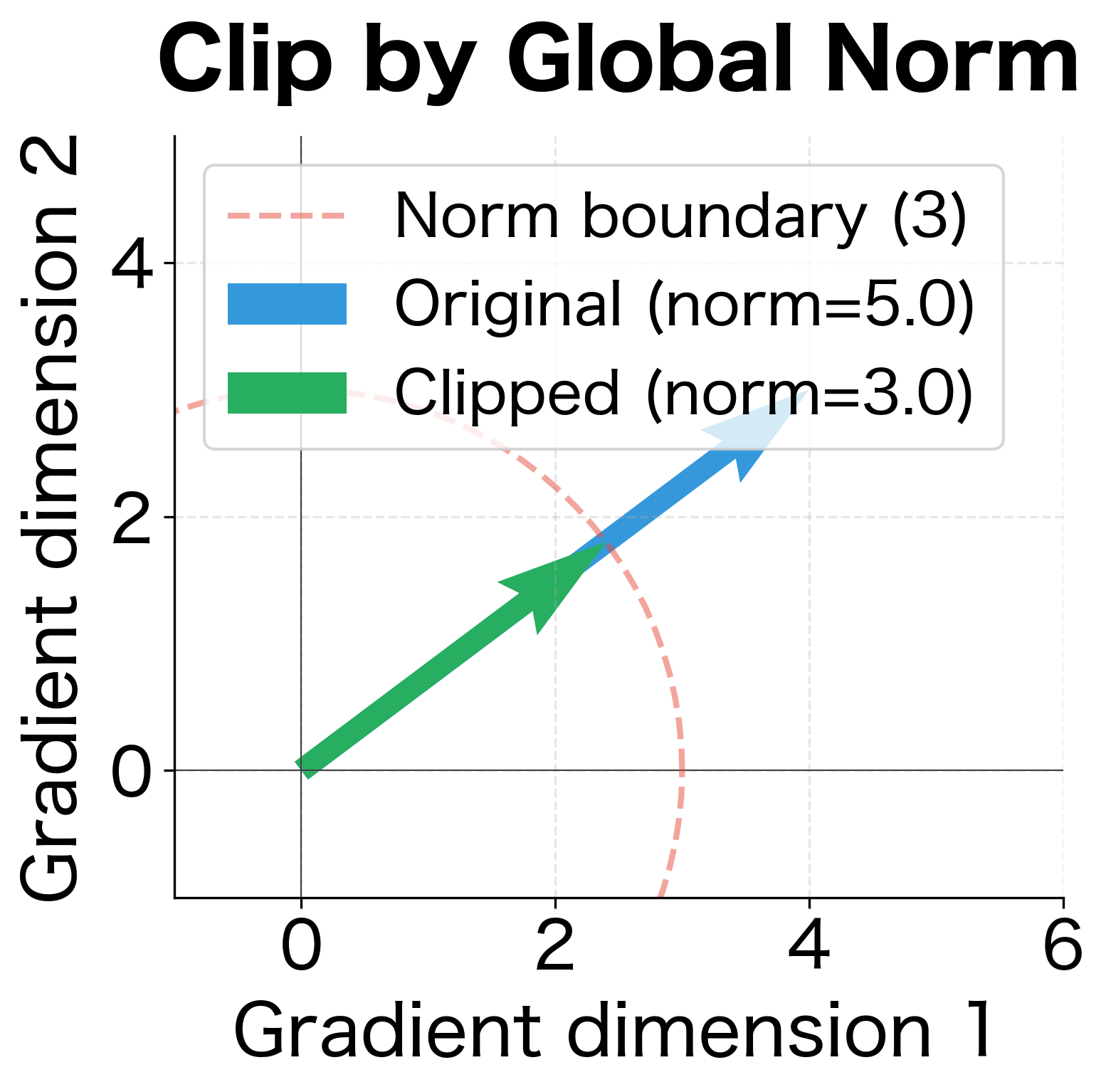
On the right, clip by norm creates a circular constraint. The same gradient $(4, 3)$ with norm 5.0 exceeds our threshold of 3.0, so we scale the entire vector by $\frac{3}{5} = 0.6$. Both components shrink proportionally to $(2.4, 1.8)$, and the angle is perfectly preserved. We're still heading in the right direction, just taking a smaller step.

This geometric intuition extends to any number of dimensions. In the parameter spaces of neural networks with millions of dimensions, clip by value constrains gradients to a hypercube while clip by norm constrains them to a hypersphere. The direction preservation property of norm clipping becomes even more valuable in high dimensions, where the corners of a hypercube can point in vastly different directions than the original gradient.

PyTorch provides built-in functions for both clipping strategies. Here's how to integrate them into a training loop.

The gradient norm determines whether clipping activates. In this case, the norm exceeds 1.0, so all gradients are scaled down proportionally. PyTorch's clip_grad_norm_ function handles this computation automatically, returning the original norm for logging purposes. The underscore suffix indicates it modifies gradients in-place.

Monitoring how often gradients get clipped provides insight into training stability. If clipping happens on every batch, your threshold might be too low. If it never happens, you might not need clipping at all.

The clipping statistics reveal training dynamics. The high initial clipping rate indicates that our threshold of 1.0 is relatively aggressive for this model, catching most gradient updates. As training progresses, gradient norms typically decrease and stabilize, leading to fewer clipping events. A healthy training run typically sees clipping on 5-20% of batches, preventing occasional spikes without constantly dampening gradients. If clipping occurs on nearly every batch, consider raising the threshold.

Plotting gradient norms over training reveals patterns that inform threshold selection. Let's train a model and visualize the gradient dynamics.

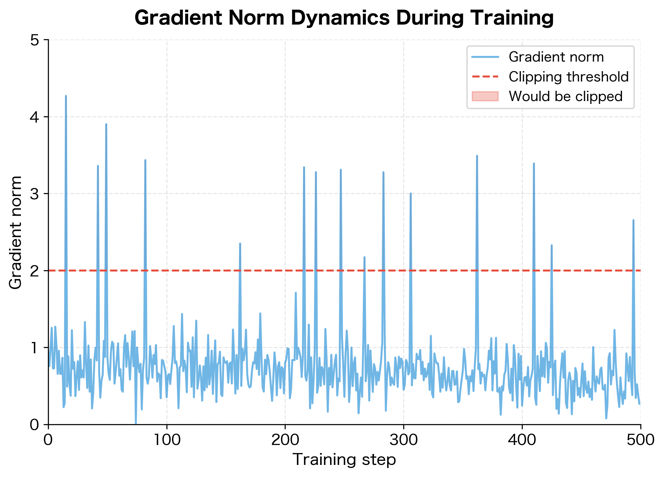
The gradient norm plot reveals the training dynamics. Early in training, gradients tend to be larger and more variable. As the model converges, gradients stabilize and shrink. The occasional spikes are the dangerous outliers that gradient clipping targets.

Selecting an appropriate clipping threshold requires balancing two concerns: clip too aggressively and you slow down learning; clip too loosely and explosions still occur.

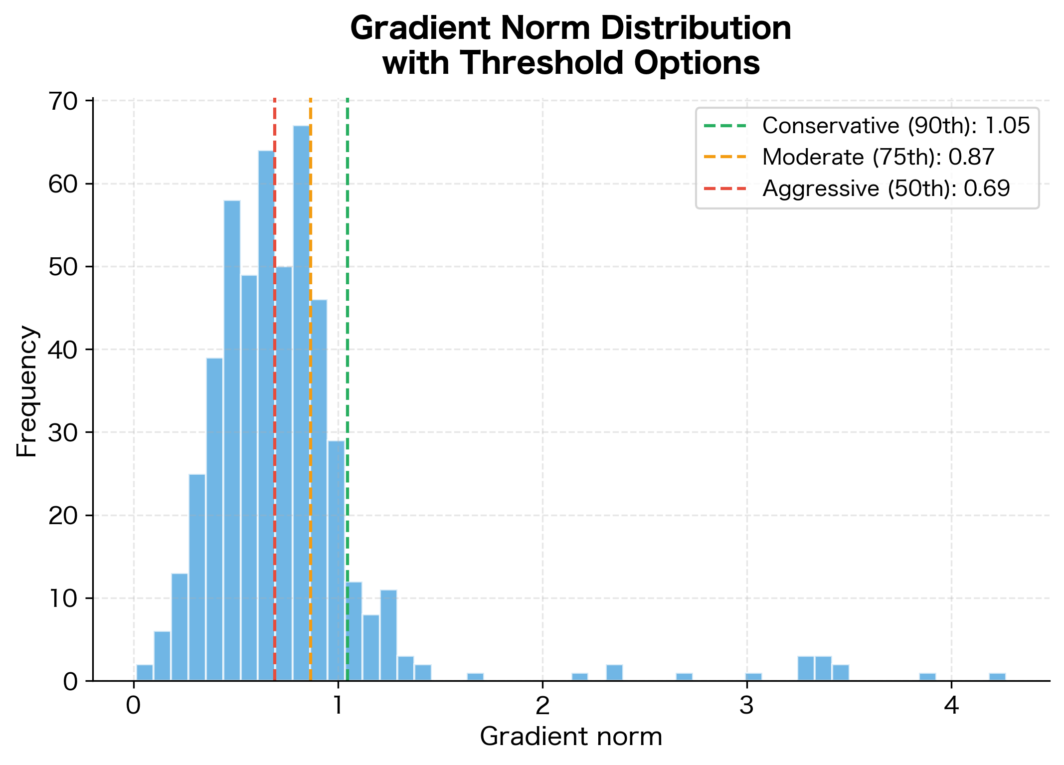
Start with a threshold based on observed gradient norms during initial training runs:

• Conservative: Set threshold at the 90th percentile of observed gradient norms. This clips only the most extreme values.
• Moderate: Use the 75th percentile. Clips more frequently but still allows most gradients through unchanged.
• Aggressive: Set threshold at the median. Halves most gradient magnitudes, useful for very unstable training.

The conservative threshold at the 90th percentile would clip only the most extreme 10% of gradients, allowing normal training dynamics while preventing outlier spikes. The moderate threshold clips about 25% of batches, providing more aggressive stabilization. The aggressive option clips half of all gradients, useful only for severely unstable training where stability matters more than convergence speed.

Certain threshold values have become standard through empirical practice:

• 1.0: A common default for transformer models. Works well with Adam optimizer and typical learning rates.
• 5.0: More permissive, used when gradients are naturally larger or training is more stable.
• 0.5: Aggressive clipping for very deep or recurrent networks with known stability issues.

The right value depends on your architecture, optimizer, and learning rate. Higher learning rates generally require lower clipping thresholds to prevent large updates.

Gradient clipping isn't always necessary. Some architectures and training setups are naturally stable, while others require careful gradient management.

The following scenarios benefit most from gradient clipping:

• Recurrent Neural Networks: LSTMs and GRUs process sequences by repeatedly applying the same weights. Long sequences create deep computational graphs prone to gradient explosion. Clipping is nearly mandatory for RNN training.
• Transformers: Self-attention mechanisms can create gradient paths that amplify through many layers. Most transformer implementations use gradient clipping by default.
• Reinforcement Learning: Policy gradients in RL can be extremely noisy and variable. Clipping stabilizes training when rewards vary dramatically.
• Large Batch Training: Gradient averaging across large batches can occasionally produce extreme values when batches contain outliers.
• Fine-tuning with High Learning Rates: When adapting pre-trained models, initial gradients can be large relative to the already-trained weights.

In some situations, gradient clipping addresses symptoms rather than causes:

• Vanishing gradients: Clipping only helps with exploding gradients. If your gradients are too small, clipping does nothing. Techniques like residual connections and layer normalization address vanishing gradients.
• Fundamentally broken architectures: If gradient explosions happen constantly and early, the architecture may need revision. Clipping is a band-aid, not a fix for poor design.
• Well-conditioned shallow networks: Simple feedforward networks with proper initialization often train stably without clipping.

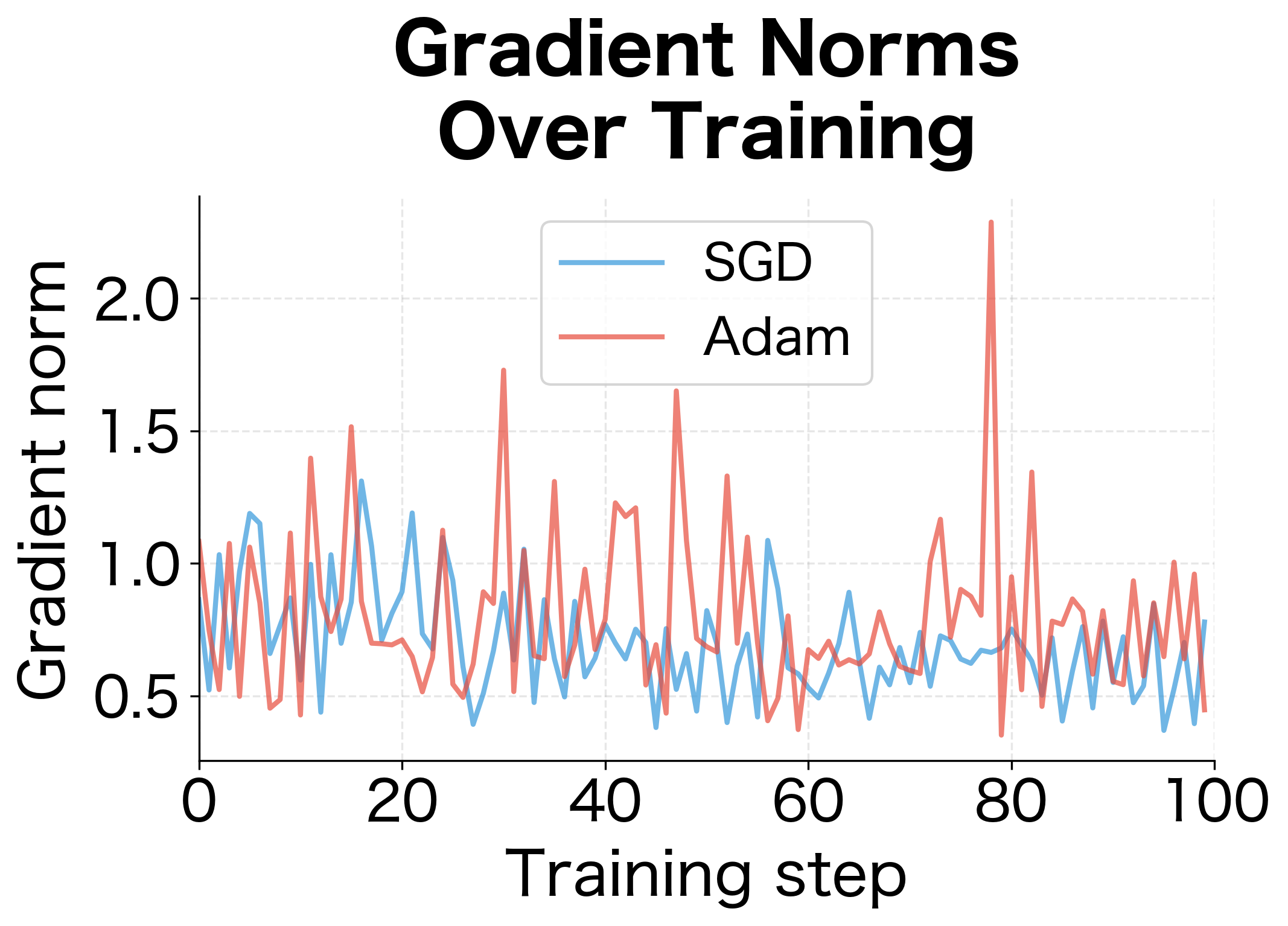
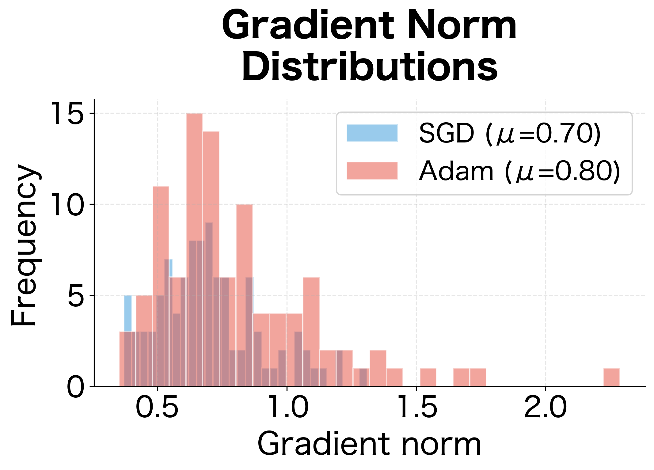
The interaction between gradient clipping and optimizers matters. Adaptive optimizers like Adam already normalize gradients per-parameter, which can reduce the need for clipping.

Both optimizers show similar gradient norm distributions since we measure gradients before the optimizer transforms them. The coefficient of variation (std/mean) indicates gradient stability. While Adam's adaptive per-parameter scaling helps with the actual updates, it doesn't change the raw gradient magnitudes that clipping operates on. For very unstable training, combining Adam with gradient clipping provides complementary stability mechanisms.

Gradient clipping is a stabilization technique, not an optimization improvement. Understanding its limitations helps you use it appropriately.

When using clip by value, we sacrifice gradient direction for bounded magnitude. This trade-off becomes more severe when gradients are highly unbalanced across dimensions. If one parameter has gradients of magnitude 100 while another has gradients of magnitude 0.1, clipping to 1.0 completely dominates the update direction toward the smaller gradient's direction. In such cases, clip by norm is strongly preferred.

Even with norm clipping, there's a subtle issue: clipping changes the effective learning rate. When gradients are clipped by a factor of 10, it's equivalent to temporarily using 1/10th of your learning rate. This can slow convergence during periods of high gradient activity, though it's usually a worthwhile trade-off for stability.

If you use learning rate warmup or decay, consider how clipping interacts with these schedules. Early in training with low learning rates, gradients might be naturally bounded. As learning rates increase during warmup, gradient clipping becomes more relevant. Some practitioners adjust clipping thresholds alongside learning rate schedules, though this adds complexity.

For production training runs, log gradient norms and clipping events. A sudden increase in clipping frequency can indicate data distribution shift, model instability, or other issues that warrant investigation. Conversely, if clipping never triggers, you might remove it to simplify your training pipeline.

When implementing gradient clipping in PyTorch, understanding the key parameters helps you configure clipping effectively for your specific training scenario:

• max_norm (for clip_grad_norm_): The maximum allowed L2 norm for the entire gradient vector. Gradients exceeding this threshold are scaled down proportionally. Common values range from 0.5 to 5.0, with 1.0 being a typical default for transformer training.

• clip_value (for clip_grad_value_): The maximum absolute value for any single gradient element. Elements outside $[-\text{clip\_value}, \text{clip\_value}]$ are clamped. Typically set higher than max_norm since it applies element-wise rather than globally.

• norm_type: The type of norm to use for clipping (default: 2 for L2 norm). Can be set to float('inf') for infinity norm or other positive values for different $p$-norms.

• error_if_nonfinite (PyTorch 1.9+): Whether to raise an error if gradients contain NaN or infinity values. Setting to True helps catch gradient explosions early rather than silently propagating corrupted values.

When selecting thresholds, start with an exploratory training run without clipping to observe your gradient norm distribution. Set the threshold at the 90th percentile for conservative clipping, or lower if training remains unstable.

Gradient clipping prevents training instability caused by exploding gradients. The technique caps gradient magnitudes before weight updates, keeping optimization on track when backpropagation produces unreasonably large values.

The key takeaways from this chapter:

• Exploding gradients occur when gradient magnitudes grow exponentially during backpropagation, especially in deep or recurrent architectures. They manifest as NaN losses and training collapse.
• Clip by value constrains each gradient element independently to $[-\tau, \tau]$, where $\tau$ is the clipping threshold. It's simple but can distort gradient direction.
• Clip by global norm rescales the entire gradient vector to have at most norm $\tau$ while preserving relative proportions. This preserves the update direction and is generally preferred.
• PyTorch's clip_grad_norm_ implements global norm clipping and is the standard choice for most applications.
• Threshold selection should be based on observed gradient norm distributions. Common values range from 0.5 to 5.0, with 1.0 being a typical default.
• Monitor clipping frequency to calibrate thresholds. Clipping on 5-20% of batches usually indicates a well-tuned threshold.

Gradient clipping is essential for training RNNs, transformers, and other deep architectures. While it doesn't improve optimization directly, it prevents the catastrophic failures that would otherwise make training impossible.

Ready to test your understanding? Take this quick quiz to reinforce what you've learned about gradient clipping and preventing exploding gradients.