CRF Training: Forward-Backward Algorithm

Conditional Random Fields are powerful models for sequence labeling, but their power comes with computational challenges. Unlike simple classifiers that make independent predictions for each token, CRFs model dependencies between labels across the entire sequence. Training a CRF means finding weights that maximize the probability of correct label sequences given their input features, while accounting for all possible alternative labelings.

To appreciate why training is non-trivial, consider what the model must accomplish. A CRF over a sentence of 20 tokens with 9 possible labels must implicitly reason over $9^{20} \approx 10^{19}$ possible label sequences every time it evaluates the probability of a correct labeling. You cannot enumerate that many sequences at training time or at prediction time. Yet somehow the model must compute, to high precision, how probable the correct sequence is relative to every alternative. That requirement is what drives the mathematical machinery covered in this chapter.

The solution comes in two steps. First, the CRF restricts how labels can depend on each other: each label may only directly influence its immediate neighbor, not arbitrary positions elsewhere in the sequence. This Markov structure means the score of any complete label sequence can be decomposed into a product of local terms. Second, the forward-backward algorithm exploits that decomposition through dynamic programming, collapsing the exponential sum into a polynomial-time computation. These two ideas together make CRF training feasible.

Once you can compute gradients efficiently, the question becomes how to optimize. The log-likelihood objective for a CRF turns out to be concave, a property that guarantees any gradient-based optimizer will find the global maximum. But gradient descent converges slowly for this class of problems. The L-BFGS optimizer, a quasi-Newton method that builds a running estimate of the objective's curvature, typically reaches the optimum in tens to a few hundred iterations rather than thousands. Understanding why L-BFGS works so well here requires understanding what makes the CRF objective well-behaved compared to neural network loss surfaces.

Feature design and regularization round out the practical picture. The CRF itself is just a scoring function; the features you feed it determine what patterns it can and cannot learn. Well-designed features encode linguistic intuitions directly, letting a small training set teach the model meaningful distinctions. Regularization prevents the optimizer from chasing statistical noise in sparse features. This ensures that learned weights generalize to new text.

This chapter explores how to train CRFs effectively. You'll learn the mathematical foundation of the log-likelihood objective, understand why the forward-backward algorithm is essential for efficient gradient computation, see how modern optimizers like L-BFGS converge faster than simple gradient descent, and discover how feature templates and regularization shape what a CRF can learn. By the end, you'll be able to train CRFs on real sequence labeling tasks and understand what's happening under the hood.

Training a CRF means finding feature weights that make correct label sequences probable. Given training data consisting of observation sequences $\mathbf{x}^{(i)}$ and their correct label sequences $\mathbf{y}^{(i)}$, we want to maximize the conditional probability of seeing these correct labels.

The key insight is that we are learning a discriminative model, not a generative one. We never model the probability of observing a particular sentence; we only model the probability of a label sequence given that sentence. This is the same philosophical stance taken by logistic regression versus naive Bayes: rather than modeling the joint distribution $P(\mathbf{x}, \mathbf{y})$, we model $P(\mathbf{y} | \mathbf{x})$ directly. For sequence labeling, this matters because modeling the sentence itself is hard (it requires a language model), while modeling labels conditioned on a sentence is much more tractable. The CRF inherits this advantage from its discriminative design.

Think of each training example as a contest between the correct label sequence and every competing alternative. The CRF assigns a score to each sequence using a weighted sum of features. Maximizing the log-likelihood of the correct sequences is equivalent to training the model to assign the correct sequence a score that is higher, on average, than the scores of all competing sequences. The partition function $Z(\mathbf{x})$ is what forces this competition: it aggregates the scores of all alternatives and normalizes them into a probability distribution. Making the correct sequence more probable necessarily means making alternative sequences less probable in relative terms.

For a single training example with observation sequence $\mathbf{x}$ and label sequence $\mathbf{y}$, the CRF defines the conditional probability as:

where:

• $\mathbf{y} = (y_1, y_2, \ldots, y_T)$: the label sequence of length $T$
• $\mathbf{x}$: the observation sequence (features at each position)
• $f_k(y_{t-1}, y_t, \mathbf{x}, t)$: the $k$-th feature function, which examines the previous label $y_{t-1}$, current label $y_t$, the full observation sequence $\mathbf{x}$, and position $t$
• $\lambda_k$: the weight for feature $k$ (what we're learning)
• $Z(\mathbf{x})$: the partition function, which sums over all possible label sequences to normalize probabilities

The partition function deserves special attention:

where:

• $\mathbf{y}'$: ranges over all possible label sequences
• The sum includes $|L|^T$ sequences, where $|L|$ is the number of possible labels

This summation over exponentially many sequences is what makes CRF training computationally interesting. With 9 labels and 20 tokens, we'd have $9^{20} \approx 10^{19}$ possible sequences. Enumerating them directly is impossible. Even if each evaluation took a nanosecond, computing the partition function by brute force would take longer than the age of the universe. The forward-backward algorithm, covered in the next section, is how we escape this combinatorial trap.

Taking the log of the conditional probability gives us the log-likelihood for a single example:

where:

• The first term is the score of the correct label sequence, a simple weighted sum of features that fire along the correct path
• The second term, $\log Z(\mathbf{x})$, is the log of the partition function and represents the log-sum-exp of scores over all possible sequences

The first term is cheap to compute: just walk along the correct label sequence and sum the feature weights at each step. The second term is the bottleneck. It requires, at least conceptually, evaluating the score of every possible label sequence and then computing a softmax-like normalization. This is where the forward-backward algorithm earns its keep.

Notice that the objective is a difference of two quantities. The first rewards the correct sequence by adding its score. The second penalizes all sequences by subtracting the log of their collective scored mass. Maximizing this difference means pushing the correct sequence score up while keeping the partition function from growing too large, which is exactly the behavior you want from a probabilistic classifier.

For the full training set with $N$ examples, we sum the log-likelihoods:

where:

• $\mathcal{L}(\boldsymbol{\lambda})$: the total log-likelihood as a function of all weights
• $\boldsymbol{\lambda} = (\lambda_1, \lambda_2, \ldots, \lambda_K)$: the vector of all $K$ feature weights

Our goal is to find $\boldsymbol{\lambda}^* = \arg\max_{\boldsymbol{\lambda}} \mathcal{L}(\boldsymbol{\lambda})$.

Let's visualize what this objective looks like for a simple case:

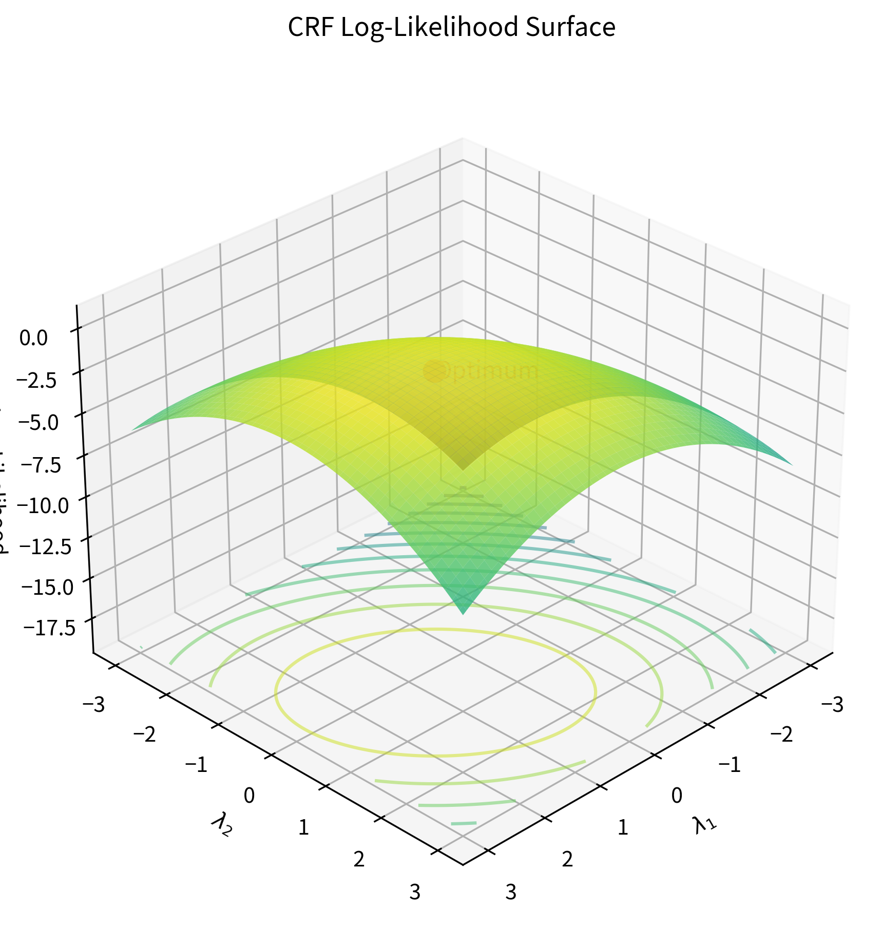
The log-likelihood function for CRFs has a important property: it is concave. This means there are no local maxima to get trapped in. Any hill-climbing algorithm will find the global optimum given enough iterations. This mathematical guarantee makes CRF training well-behaved compared to neural network training, where the loss surface contains local minima and saddle points.

The concavity follows from the log-sum-exp structure of the partition function. The log-sum-exp of linear functions is convex, so subtracting it from a linear function yields a concave result. In practice, this means you can initialize weights to zero and trust that any reasonable optimizer will converge to the same solution regardless of starting point. When your CRF training converges poorly, the culprit is almost always numerical issues, inappropriate learning rates, or degenerate features rather than getting stuck in a bad local optimum.

Computing the partition function $Z(\mathbf{x})$ by enumerating all sequences is intractable. The forward-backward algorithm exploits the sequential structure of the model to compute it in polynomial time.

The key insight is that the CRF score decomposes into local terms. At each position $t$, the contribution depends only on the label at $t$ and the label at $t-1$. This Markov property enables dynamic programming: we can build up the sum over all sequences incrementally, position by position.

Think of the forward-backward algorithm as a two-pass bookkeeping system for computing partial sums efficiently. The forward pass sweeps left to right, and at each position it records the total score of all partial paths that end at that position with each possible label. The backward pass sweeps right to left and records the total score of all partial paths that extend from each position to the end. When you multiply the forward score at a node with its backward score, you get the total score of all complete paths that pass through that node. This product is proportional to the marginal probability of being in that state at that position.

The algorithm draws its name and structure from the forward-backward algorithm for Hidden Markov Models, which you may have encountered in the previous chapter on HMMs. The CRF version works the same way conceptually, but in log space to avoid numerical underflow when sequences grow long. In practice, working in log space converts multiplications into additions and uses the log-sum-exp trick to combine scores safely. The transition from probability space to log space is a consistent theme in modern sequence modeling, and it applies here with the same motivation: multiplying many small probabilities together quickly produces values too tiny for floating-point arithmetic to represent accurately.

Think of the forward variable as an accumulator. As you sweep through the sequence from left to right, the forward variable at each position records everything you need to know about paths that have arrived at each possible label state. You never need to remember which specific path got you there, only the total aggregated score of all such paths. This is the essence of dynamic programming: discard the details, keep the aggregate.

The forward variable $\alpha_t(j)$ represents the sum of scores for all partial label sequences that end with label $j$ at position $t$:

where:

• $\mathbf{y}_{1:t}$: all possible label sequences from position 1 to $t$
• $y_t = j$: constrained to end with label $j$
• The summation accumulates scores of all paths reaching state $j$ at time $t$

We compute forward variables recursively:

Base case (t = 1):

where $y_0$ is a special start symbol.

Recursive case:

This recursion says: to get the total score of paths ending in $j$ at position $t$, sum over all possible previous labels $i$, multiplying the forward score at $t-1$ (all paths ending in $i$) by the transition score from $i$ to $j$.

Notice that the recursion reuses the previous time step's forward variables rather than recomputing everything from scratch. Each $\alpha_t(j)$ requires only the $|L|$ values from $\alpha_{t-1}(\cdot)$, so the total storage is $O(T \cdot |L|)$ and the total computation is $O(T \cdot |L|^2)$: for each of $T$ positions and each of $|L|$ possible current labels, we sum over $|L|$ possible previous labels. This is a dramatic improvement over the $O(|L|^T)$ cost of brute-force enumeration.

The partition function is simply the sum of all forward variables at the final position:

The backward variable is symmetric to the forward variable but runs in the opposite direction. While the forward variable answers "what is the total score of all paths that reach state $i$ at position $t$ coming from the left?", the backward variable answers "what is the total score of all paths that extend from state $i$ at position $t$ to the right end of the sequence?" Together, a forward value and a backward value bracket a specific state at a specific position, and their product gives the total score of all complete paths that pass through that state.

The backward variable $\beta_t(i)$ represents the sum of scores for all partial sequences starting from position $t+1$, given that position $t$ has label $i$:

where $y_t = i$ is fixed.

Base case (t = T):

Recursive case:

The forward and backward variables together give us the probability of any label at any position. In practice, this is why we run both passes: the forward pass alone gives us the partition function, but both passes together give us the full set of marginal probabilities that we need for gradient computation. The posterior marginal probability of label $j$ at position $t$ is:

And the probability of a specific transition from $i$ to $j$ at positions $t-1$ to $t$:

where $M_t(i, j) = \exp\left(\sum_k \lambda_k f_k(i, j, \mathbf{x}, t)\right)$ is the transition score matrix at position $t$.

Let's implement the forward-backward algorithm:

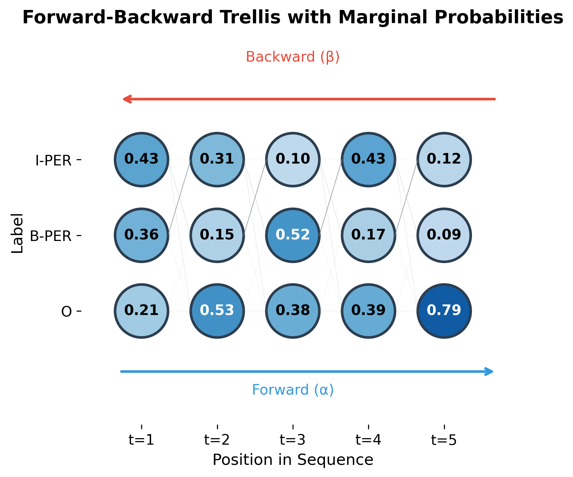
The trellis visualization shows how forward and backward passes combine. Each node's color intensity represents its marginal probability. States with high marginal probability (darker blue) are more likely to be part of the optimal sequence.

To optimize the log-likelihood, we need its gradient with respect to each weight $\lambda_k$. The gradient has an elegant form that emerges from the structure of the CRF, and understanding this form gives deep insight into what training accomplishes.

Taking the derivative of the log-likelihood for a single example:

where:

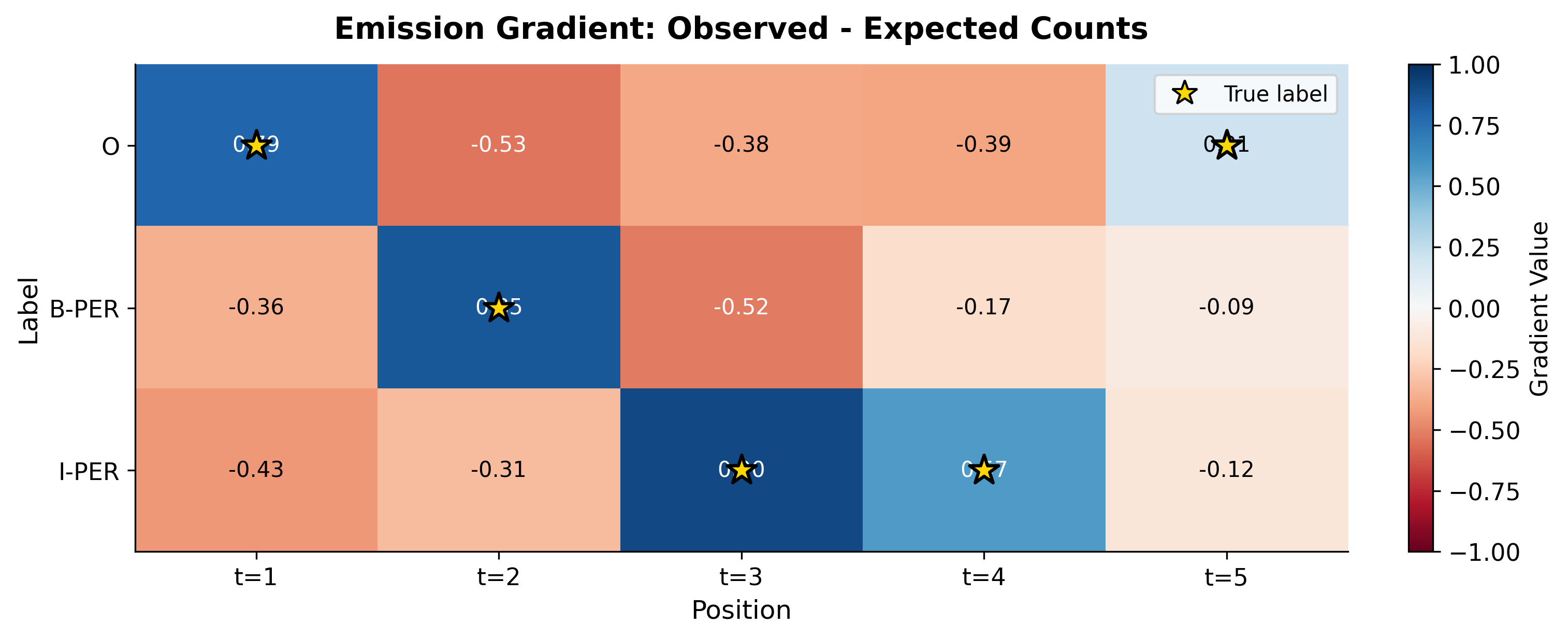
• The first term is the observed feature count: how often feature $k$ fires on the correct label sequence
• The second term is the expected feature count: the expected number of times feature $k$ would fire under the model's current probability distribution

This gradient has an intuitive interpretation:

• If a feature fires more often in the training data than the model expects, increase its weight (positive gradient)
• If a feature fires less often than expected, decrease its weight (negative gradient)
• When observed counts match expected counts, the gradient is zero (we've reached a stationary point)

The key insight is that the gradient is a simple difference: observed minus expected. This mirrors the gradient of logistic regression and maximum entropy models. In fact, you can view CRF training as a natural generalization of logistic regression to structured outputs: instead of matching observed class frequencies with expected class frequencies, you match observed feature counts along label sequences with expected feature counts under the model's current distribution.

The elegance of this formulation makes the convergence criterion transparent. You know the model has converged when, for every feature, the number of times it fires in the training data equals the number of times the model expects it to fire. This is a moment-matching condition, and it has a beautiful statistical interpretation: the model has learned to reproduce the sufficient statistics of the training data under its own probability distribution.

This has a practical consequence. Features that are rare in the training data will have noisy observed counts, which means their gradients are noisy too. A feature that fires exactly once in a large dataset has an observed count of 1 and a very uncertain expected count. Regularization, which we cover later, is partly a response to this noise: by penalizing large weights, it prevents the optimizer from placing too much confidence in observations from very rare features.

The expected feature count requires summing over all positions and all label pairs, weighted by their posterior probabilities. This is where the pairwise marginals come in:

where:

• $P(y_{t-1} = i, y_t = j | \mathbf{x})$: the posterior probability that the label pair $(i, j)$ occurs at positions $t-1$ and $t$, marginalized over all other positions
• $f_k(i, j, \mathbf{x}, t)$: the value of feature $k$ when the previous label is $i$, the current label is $j$, and we are at position $t$

The forward-backward algorithm gives us exactly what we need: the pairwise marginals $P(y_{t-1} = i, y_t = j | \mathbf{x})$. Each call to forward-backward for a single training example produces all the information needed to compute the gradient contribution from that example. This is computationally efficient: rather than running a separate algorithm for inference and a separate algorithm for gradient computation, the forward-backward algorithm serves both purposes simultaneously.

Simple gradient descent can optimize the CRF objective, but it converges slowly. Each step moves in the direction of the gradient, but the step size is tricky to tune: too large and you overshoot, too small and you crawl toward the optimum.

L-BFGS (Limited-memory Broyden-Fletcher-Goldfarb-Shanno) is a quasi-Newton method that approximates the curvature of the objective function. Instead of using only the gradient direction, it uses gradient history to estimate how the objective curves in different directions, enabling larger steps in flat directions and smaller steps in steep directions.

To understand why L-BFGS converges faster than gradient descent, consider what the Hessian tells you. The Hessian matrix of second derivatives describes the curvature of the objective in every direction. Directions with high curvature (large second derivatives) require small steps to avoid overshooting; directions with low curvature (small second derivatives) can tolerate large steps. Gradient descent uses the same step size (or a line-searched step size) in all directions, which means it is either too aggressive in high-curvature directions or too conservative in low-curvature ones. By approximating the inverse Hessian, L-BFGS can scale each direction appropriately, taking large steps in flat directions and small steps in steep ones. This is the key reason it converges in far fewer iterations.

For CRF training specifically, the curvature of the log-likelihood objective depends on the feature correlations in the training data. Features that are highly correlated with each other create directions of low curvature that gradient descent handles poorly. L-BFGS handles this naturally by building up an estimate of these correlations over iterations.

The key advantages of L-BFGS for CRF training are:

• Faster convergence: Uses curvature information to take better steps
• No learning rate tuning: Line search automatically finds good step sizes
• Memory efficient: Stores only the last $m$ gradient pairs (typically $m = 10$), not the full Hessian
• Stable: Works well on the convex CRF objective without careful hyperparameter tuning

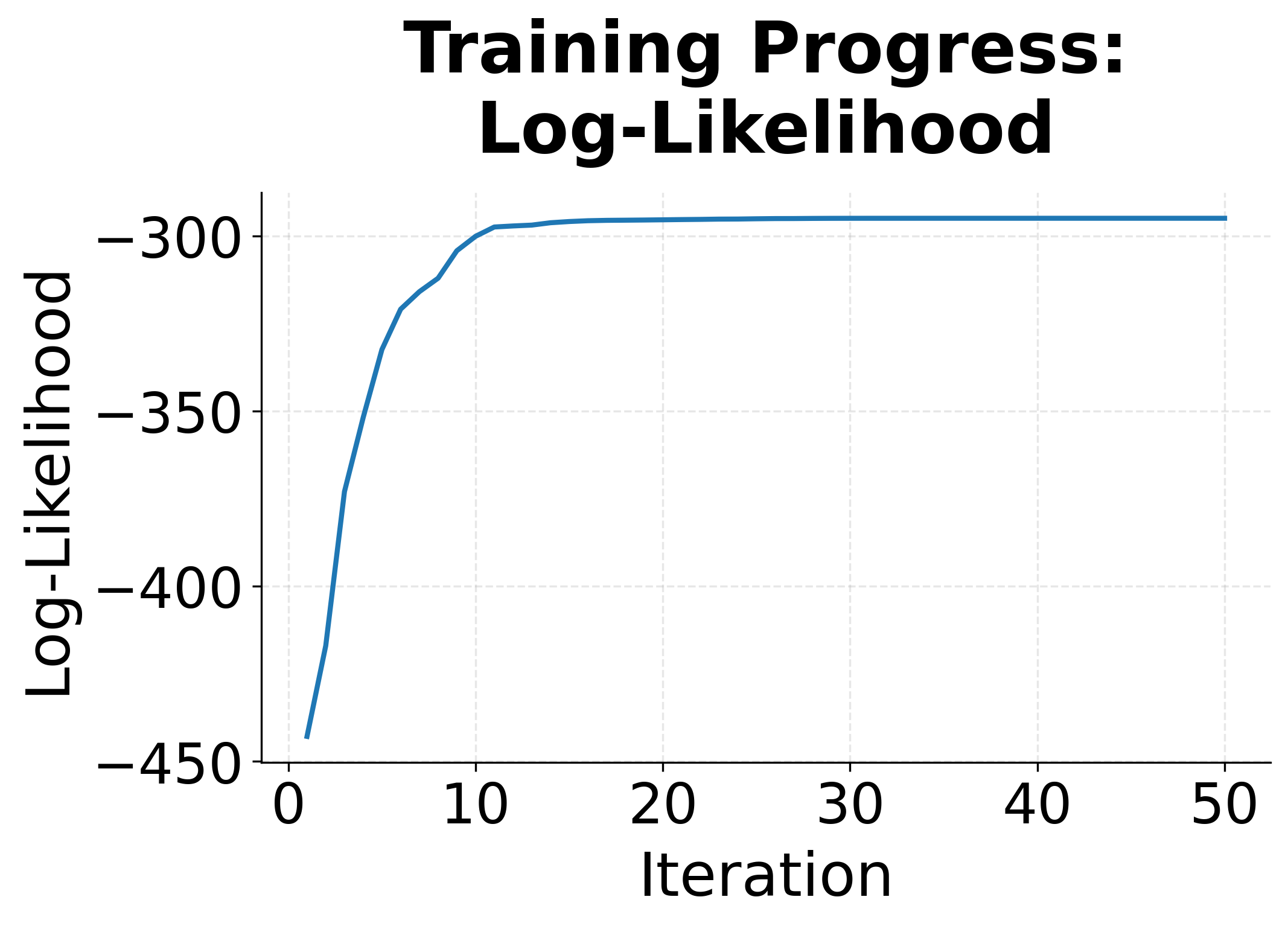
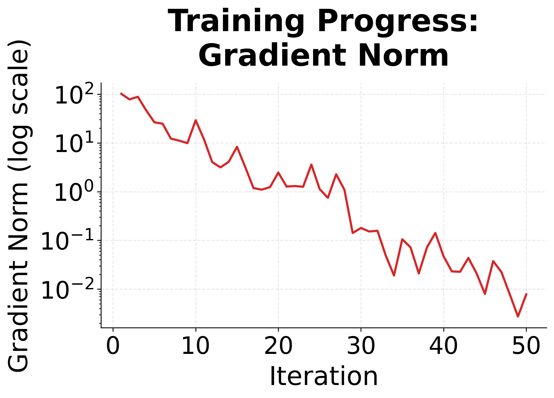
The convergence plots show the characteristic behavior of L-BFGS on a convex problem. The log-likelihood rises steeply at first, then levels off as we approach the optimum. The gradient norm drops exponentially, indicating we're getting closer to a point where the gradient is zero.

Notice that the gradient norm does not decrease monotonically at each step. L-BFGS performs a line search along the descent direction computed from the approximate inverse Hessian, and this line search may occasionally accept a step that temporarily increases the gradient norm. This is normal and expected: the optimizer is exploring the curvature structure of the objective in order to build a better approximation. Over a window of several iterations, the trend should be consistently downward.

In practice, L-BFGS convergence on a well-conditioned CRF typically takes 50 to 200 iterations. The exact count depends on the number of training examples, the number of features, and the regularization strength. Stronger regularization generally leads to faster convergence because it smooths the objective and reduces the condition number of the Hessian. If your CRF training is taking thousands of iterations to converge, suspect either a very large feature set with many correlated features, a very small regularization coefficient, or numerical issues in the gradient computation.

CRF features are the heart of the model. Well-designed features capture the patterns that distinguish correct label sequences from incorrect ones. Feature templates define how to extract features from the input, and the CRF learns which features matter most.

The distinction between a feature template and a feature instance matters. A template like "current word = X" is a recipe that generates thousands of concrete features, one for each vocabulary word. You define the template once; the feature extraction code instantiates all the concrete features automatically when it encounters each word in the training data. This design is elegant because it allows the feature set to scale with the vocabulary without requiring you to enumerate every possible feature in advance.

Feature design for CRFs is both an art and an empirical practice. The goal is to encode enough signal that the CRF can distinguish between correct and incorrect label assignments, without being so redundant or noisy that the model overfits to training artifacts. A useful mental model is to think about what a linguistically informed human annotator would notice when deciding on a label. If a feature captures something that a human would use as evidence, it is probably worth including. If it captures something accidental about the training data, it will hurt generalization.

Features for sequence labeling typically fall into several categories:

• Lexical features: The word itself, lowercase form, word shape (capitalization pattern)
• Contextual features: Surrounding words in a window
• Morphological features: Prefixes, suffixes, presence of digits or punctuation
• Part-of-speech features: POS tags from a tagger (if available)
• Transition features: Combinations of previous and current labels

Each category captures a different kind of evidence. Lexical features are the most direct: the word "London" is almost always a location. But lexical features are also the most data-hungry: to learn that "London" is a location, the model needs to see it in training data. Morphological features generalize better because they fire for unseen words: a word ending in "-shire" is probably a British county even if the specific word never appeared in training. Context features capture relational information: a capitalized word immediately after "President" is likely a person's name.

The most powerful features are often combinations: "the previous word is 'Dr.' and the current word is capitalized" is a much stronger signal for a person name than either feature alone. CRFs can represent such combinations as conjunctive features, and many feature engineering libraries automatically generate pairwise combinations of base features to capture these interactions.

The feature extractor captures patterns that are predictive of entity labels. Title-cased words are often names. Words ending in "-ia" might be locations. Words preceded by "at" might be organizations. The CRF learns which of these patterns are reliable predictors.

One thing to notice about the feature extractor above is that it uses the raw word itself as one of the features. This creates one binary feature per unique word in the vocabulary, and those features will have zero weight for any word not seen in training. This is the "unknown word" problem, and it is one of the fundamental challenges in classical NLP. Morphological features like prefixes and suffixes partially address it: even an unseen word shares its suffix with many seen words, allowing the model to make reasonable guesses. Treating unknown words as a special token is another common approach, at the cost of losing information about what the unknown word looks like.

Real NER systems use extensive feature templates. The richness of the feature set often matters more than the choice of optimizer or regularization strength. McCallum and Li's influential 2003 paper on CRF-based NER used over 100,000 features on the CoNLL 2003 benchmark, carefully designed to capture capitalization, word shapes, gazetteers of known names, and contextual patterns from several words before and after each token. At the time, this was state of the art for English NER.

The sklearn-crfsuite library provides a convenient way to train CRFs with custom features:

The learned feature weights reveal what the CRF considers important. High positive weights for "word.istitle=True" on B-PER indicate that title-cased words are strong signals for person names. The CRF automatically discovers these patterns from the training data.

Inspecting feature weights is one of the most valuable diagnostic tools for CRF practitioners. Unlike neural networks, where the learned representations are distributed and opaque, CRF weights are directly interpretable: each weight has a straightforward meaning as the log-odds contribution of that feature to that label. A large positive weight for "word[-3:]=ian" on I-PER means the model has learned that words ending in "-ian" (like "Iranian" or "Brazilian") often appear inside person entity spans. A large negative weight for the same feature on B-ORG means such words are unlikely to start organization spans. Debugging a CRF that makes systematic errors often starts with examining the weights of features that seem relevant to the error type.

Without regularization, CRF training can overfit to the training data. If a feature appears only once in training and perfectly predicts a label, the optimal weight is infinity. Regularization prevents extreme weights and improves generalization.

To understand why CRFs need regularization, consider what happens with a feature like "word=Schenectady" that fires exactly once in the training data, where the word was labeled B-LOC. If we maximize log-likelihood without any penalty, the optimal weight for this feature approaches infinity: making that weight arbitrarily large makes the CRF assign arbitrarily high probability to labeling "Schenectady" as B-LOC, which perfectly explains the one training example. But at test time, if the model sees "Schenectady" in a context where it is labeled differently (perhaps in a business name), the overly large weight will cause errors.

Regularization resolves this by adding a cost for large weights. The optimizer must balance two competing objectives: maximize the fit to training data, and keep weights small. For features that appear only once or twice, the training data provides weak evidence, so the optimizer accepts some loss in training fit to keep the weight reasonable. For features that appear hundreds of times with consistent labels, the training signal is strong enough to overcome the regularization cost, and the weight grows to reflect the recurring pattern.

The regularized log-likelihood objective is:

where:

• $\mathcal{L}(\boldsymbol{\lambda})$: the original log-likelihood
• $C_1$: L1 regularization coefficient (larger = less regularization)
• $C_2$: L2 regularization coefficient (larger = less regularization)
• $|\lambda_k|$: absolute value of weight $k$ (L1 penalty)
• $\lambda_k^2$: squared weight (L2 penalty)

L1 and L2 regularization have different effects:

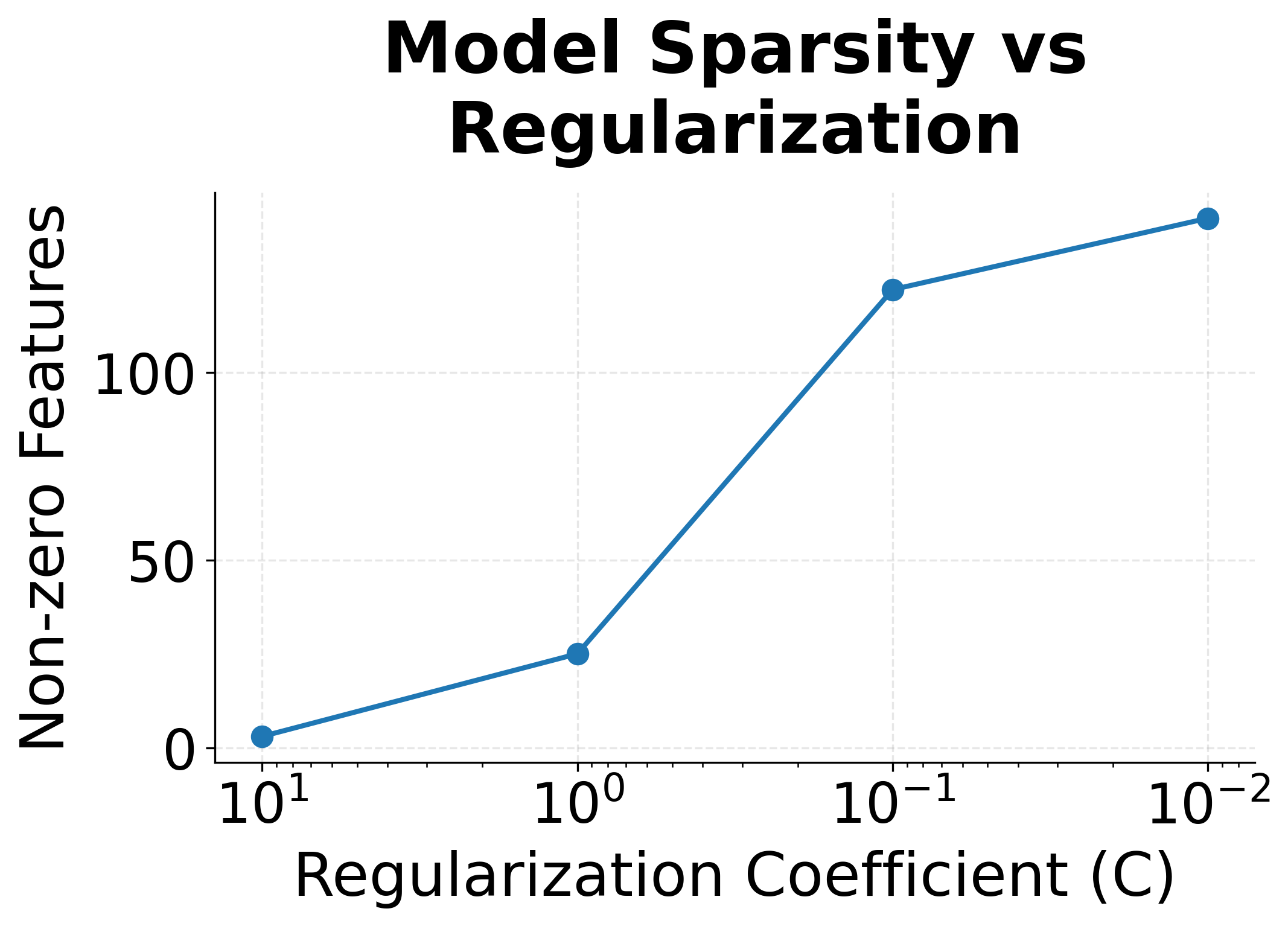
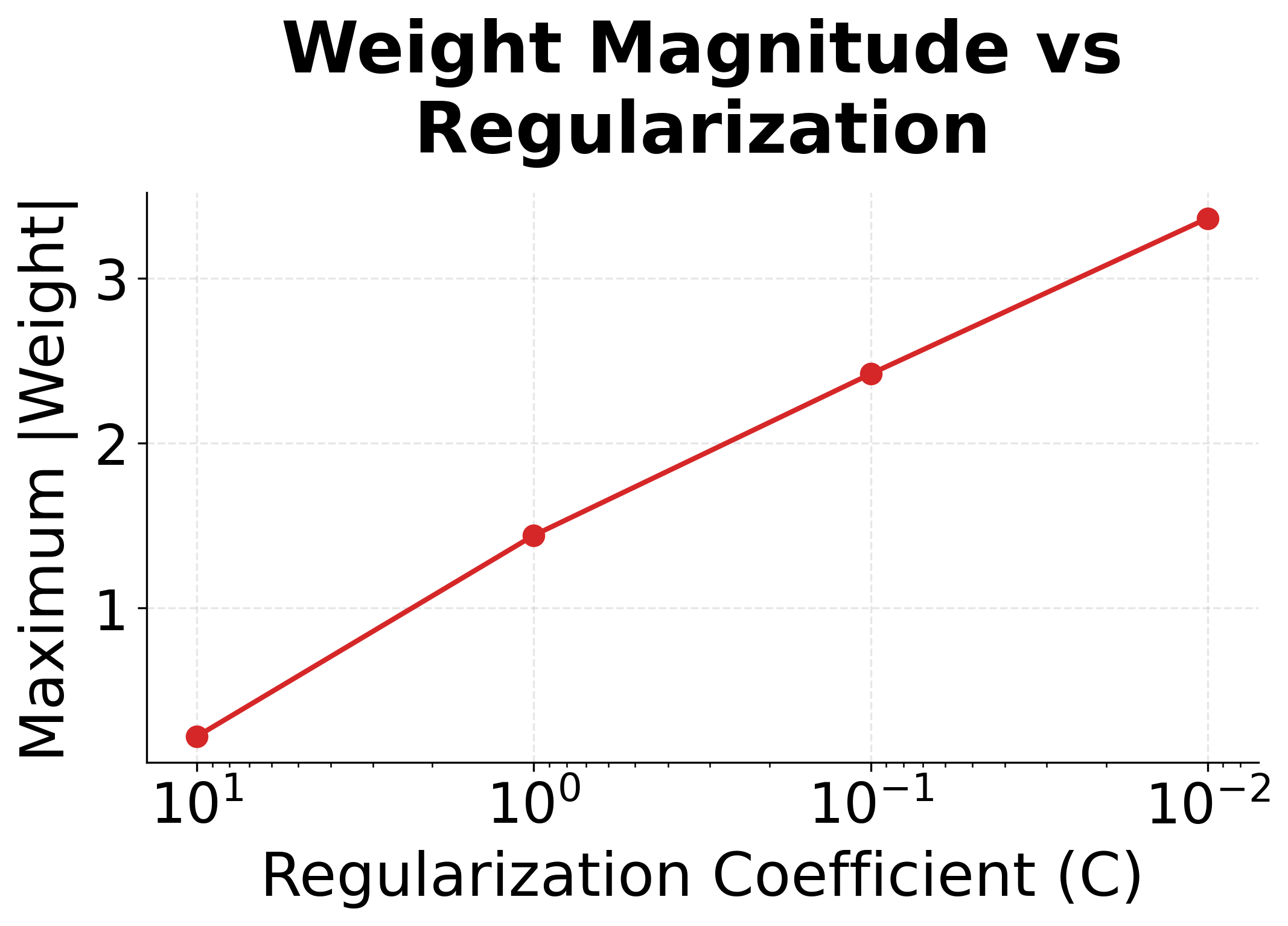
The regularization plots show clear trends. With strong regularization (small C), many features get zeroed out, creating a sparse model that uses only the most informative features. Maximum weight magnitudes also decrease, preventing the model from over-relying on any single feature.

Choosing the right regularization strength is a hyperparameter tuning problem. The common practice is to try a geometric grid of values, such as $C \in \{0.01, 0.03, 0.1, 0.3, 1.0\}$, and evaluate each on a held-out development set using the F1 score or other task-specific metric. For NER, the metric of interest is usually entity-level F1, which requires predicting both the boundary and the type of each entity correctly. A regularization coefficient that maximizes token-level accuracy might produce many boundary errors; measuring F1 at the entity level is more informative for the deployment use case.

In practice, L2 regularization ($c_2$) is the safer default choice because it does not produce discontinuous gradients. L1 regularization produces a gradient discontinuity at zero: the subgradient at $\lambda_k = 0$ is not unique, which requires special handling in gradient-based optimizers. L-BFGS in scipy handles L1 via the OWL-QN extension, which operates on the L-BFGS-B variant. The key practical difference is that L1 often produces better-compressed models (many exact zeros) while L2 tends to produce models where all features have small nonzero weights. For deployment scenarios where model size or inference speed matters, L1 or combined L1+L2 may be preferable despite the added optimization complexity.

Let's put everything together and train a CRF on a real NER dataset. This section is both a demonstration of the full pipeline and a worked example of how the concepts from earlier sections appear in a practical setting. the training loop implicitly performs the forward-backward pass for each sentence during each L-BFGS iteration, how the regularization parameters shape the learned feature weights, and how the transition matrix encodes the label structure of the NER task.

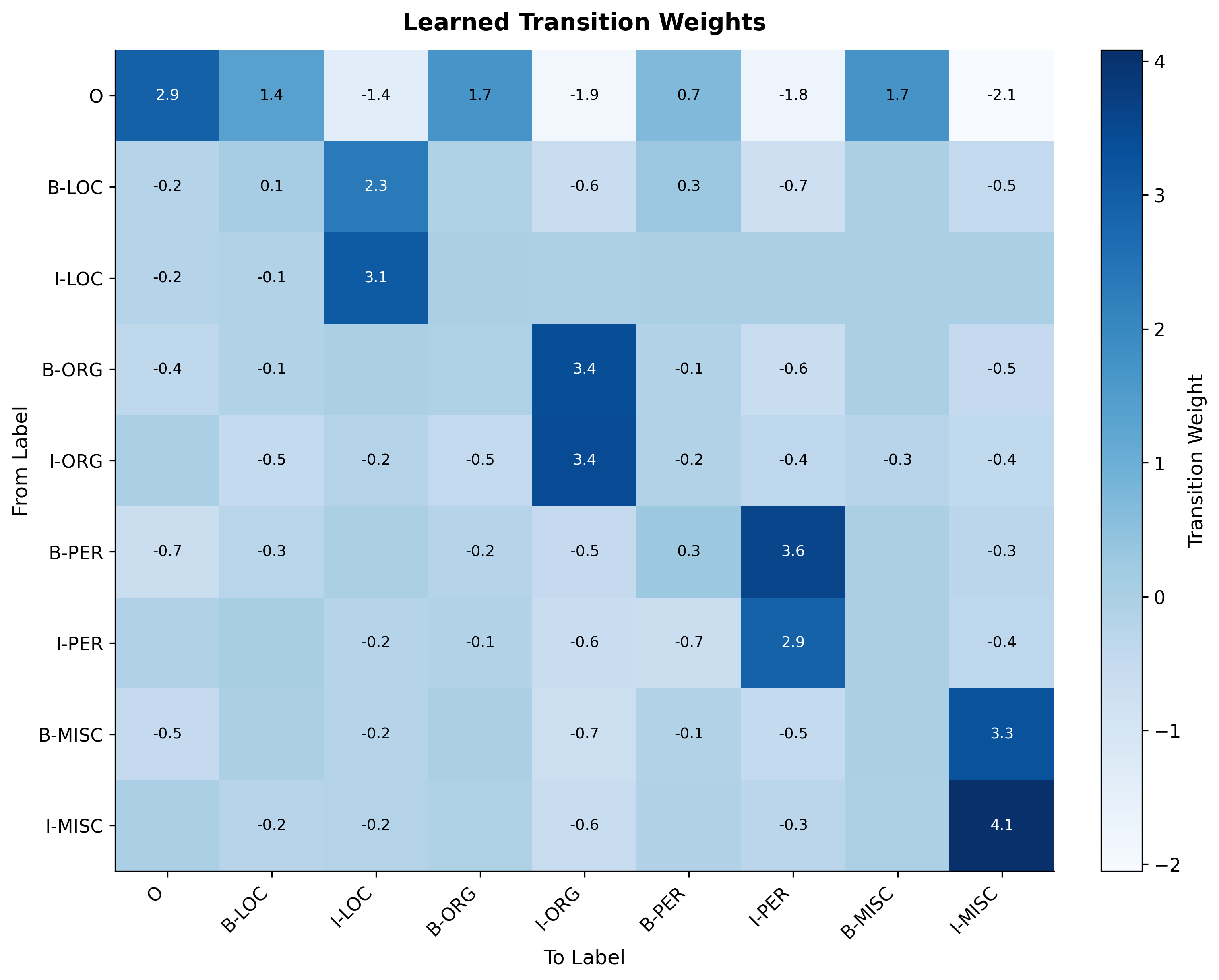
The transition matrix reveals that the CRF has learned BIO constraints. High weights appear for valid transitions like O→B-LOC (starting a location entity) and B-LOC→I-LOC (continuing a location). Low or negative weights appear for invalid transitions like O→I-LOC (continuation without a beginning).

This automatic discovery of BIO constraints is one of the most useful practical advantages of CRFs over independent classifiers. A per-token classifier trained to predict NER labels will sometimes predict I-PER at the start of a sentence, which violates the BIO convention and is meaningless. The CRF cannot make that mistake: the learned transition weight from O (or from the start symbol) to I-PER will be strongly negative, because the training data never contains such a transition. The model is implicitly learning the structural rules of the tagging scheme from examples, without needing those rules to be hard-coded.

An important nuance: the CRF only learns BIO constraints as soft preferences, not hard rules. If the evidence from the emission features is strong enough (e.g., the word strongly looks like it continues an entity), the model can still produce invalid BIO sequences when the transition cost does not overwhelm the emission score. Some practitioners handle this by using a post-processing step that converts CRF output to valid BIO sequences, or by using a constrained Viterbi decoding that enforces hard BIO constraints during inference.

CRF training has both strengths and limitations that shape when and how to use these models effectively.

The forward-backward algorithm makes CRF training tractable, but it still requires $O(T \cdot |L|^2)$ time per sequence. For tasks with many labels like fine-grained NER or semantic role labeling, this quadratic scaling becomes expensive. A sequence with 50 labels and 100 tokens requires computing 250,000 transition scores per training example. This cost compounds across thousands of training sentences and hundreds of optimization iterations. For real-time applications or very large training corpora, even this polynomial cost can become a bottleneck, and practitioners sometimes turn to approximate inference methods or batch the training examples to exploit parallelism.

Feature engineering remains both a strength and weakness. Hand-crafted features like word shapes, prefixes, and context windows capture linguistic knowledge effectively. But designing features requires domain expertise and extensive experimentation. Features that work well for English NER may perform poorly on German or Japanese: German capitalizes all nouns, so capitalization is a weaker signal for named entities; Japanese has no spaces between words, making the notion of a "word" itself a pre-processing challenge. Adapting a CRF to a new language or domain often requires redesigning the feature set from scratch, which is time-consuming and requires linguistic knowledge of the target language.

CRFs also struggle with long-range dependencies. The Markov assumption means each label depends only on the immediately preceding label. If a token's correct label depends on context five words away, the CRF must propagate that information through intervening transitions. In practice, this limits how much global context the model can exploit. You can partially compensate by including context features that look several words in either direction, but these are fixed features rather than learned representations, so they cannot capture the full richness of long-range dependencies.

Another fundamental limitation is the inability to handle overlapping entities. Standard CRFs produce exactly one label per token, so they cannot represent the case where "New York City" is simultaneously a location and part of an organization name. More complex models like semi-CRFs or factorial CRFs address some of these limitations but at greater computational cost.

Despite these limitations, CRFs made sequence labeling practical before deep learning. Their contribution extends beyond the models themselves to the training paradigms they established. The idea of discriminatively training structured models, using dynamic programming for efficient inference, and designing features to capture domain knowledge influenced subsequent developments in neural NLP. Modern neural CRF layers, which place a CRF on top of BiLSTM or transformer encoders, combine learned representations with the structured prediction framework that CRFs pioneered. When you use a BERT-based NER model with a CRF output layer today, you are using a direct descendant of the approach described in this chapter.

For practitioners today, CRFs remain valuable in several scenarios. When training data is limited (hundreds rather than thousands of examples), CRFs often outperform neural models because their features encode prior knowledge that the neural model cannot learn from a small sample. When interpretability matters, examining feature weights reveals what the model has learned in terms a domain expert can evaluate and critique. When computational resources are constrained, CRFs train on CPUs in minutes rather than requiring GPUs for hours. And as components in hybrid systems, CRF output layers on top of neural encoders often improve boundary accuracy compared to using softmax alone, because they enforce global consistency across the label sequence.

The historical importance of CRFs also lies in what they taught the NLP community about structured prediction. Before CRFs, many NLP systems used pipeline architectures: a POS tagger trained independently, then an NER model trained independently using POS tags as features. CRFs enabled joint training, where the output structure itself is modeled as a random variable and the model is optimized end-to-end over the full output. This shift from pipeline to joint modeling was one of the conceptual breakthroughs that set the stage for the end-to-end neural models that came later.

Training Conditional Random Fields requires balancing computational efficiency with model expressiveness. The chapter covered each of the key components that make CRF training work in practice.

The log-likelihood objective is the foundation: CRF training maximizes the probability of correct label sequences. The objective is concave, guaranteeing a unique global optimum without the pathological local minima that complicate neural network training. This concavity follows from the log-sum-exp structure of the partition function and makes CRFs one of the most theoretically clean models in NLP.

The forward-backward algorithm is the computational engine. Dynamic programming computes the partition function and all marginal probabilities in $O(T \cdot |L|^2)$ time, making training tractable despite the exponential number of possible label sequences. The algorithm runs in log space to avoid numerical underflow, using the log-sum-exp trick at each step. Both forward and backward passes are required: the forward pass alone gives the partition function, but both together give the pairwise marginals needed for gradient computation.

Gradient computation follows directly from the forward-backward pass. The gradient equals observed feature counts minus expected feature counts. This moment-matching interpretation makes the convergence criterion transparent: training is complete when the model's distribution over label sequences reproduces the empirical feature statistics of the training data, subject to the regularization constraint.

L-BFGS optimization closes the loop between gradient computation and weight updates. Quasi-Newton methods converge much faster than gradient descent by approximating curvature information from gradient history. Most CRF implementations use L-BFGS by default because the convex CRF objective is well-suited to second-order methods and does not require the careful learning rate scheduling that gradient descent demands.

Feature templates encode domain knowledge into the model. Hand-designed features capture patterns like word shapes, context windows, morphological properties, and neighboring POS tags. Good feature design is often more important than optimizer choice or regularization strength, because the CRF can only learn patterns that the features can represent.

Regularization prevents overfitting by penalizing large weights. L1 regularization (c1 in sklearn-crfsuite) produces sparse models by driving many weights to exactly zero. L2 regularization (c2) shrinks all weights toward zero without enforcing sparsity. In practice, a small amount of both is often most effective. Regularization strength should be chosen by cross-validation on a development set.

CRFs established the foundation for structured prediction in NLP. While neural approaches now dominate many leaderboards, the principles of discriminative training, dynamic programming, and structured output remain central to modern sequence labeling systems. Neural CRF models directly inherit this framework, placing the CRF training objective on top of learned feature representations. Understanding how CRFs are trained makes these modern hybrid models much easier to reason about and debug.

Ready to test your understanding? Take this quick quiz to reinforce what you've learned about CRF training.