

Learn why weight initialization matters for training neural networks. Covers Xavier and He initialization, variance propagation analysis, and practical PyTorch implementation.

This article is part of the free-to-read Language AI Handbook
Choose your expertise level to adjust how many terms are explained. Beginners see more tooltips, experts see fewer to maintain reading flow. Hover over underlined terms for instant definitions.
Weight Initialization
Training a neural network means finding good values for its weights, but where do we start? The answer matters more than you might expect. If we initialize weights poorly, gradients can explode to infinity or vanish to zero, making learning impossible before it even begins. The right initialization sets the stage for stable, efficient training.
This chapter explores why weight initialization matters and how techniques like Xavier and He initialization solve the problems that plagued early deep networks. We'll derive these methods from first principles, implement them from scratch, and see how they enable training networks that would otherwise fail to learn.
The Need for Careful Initialization
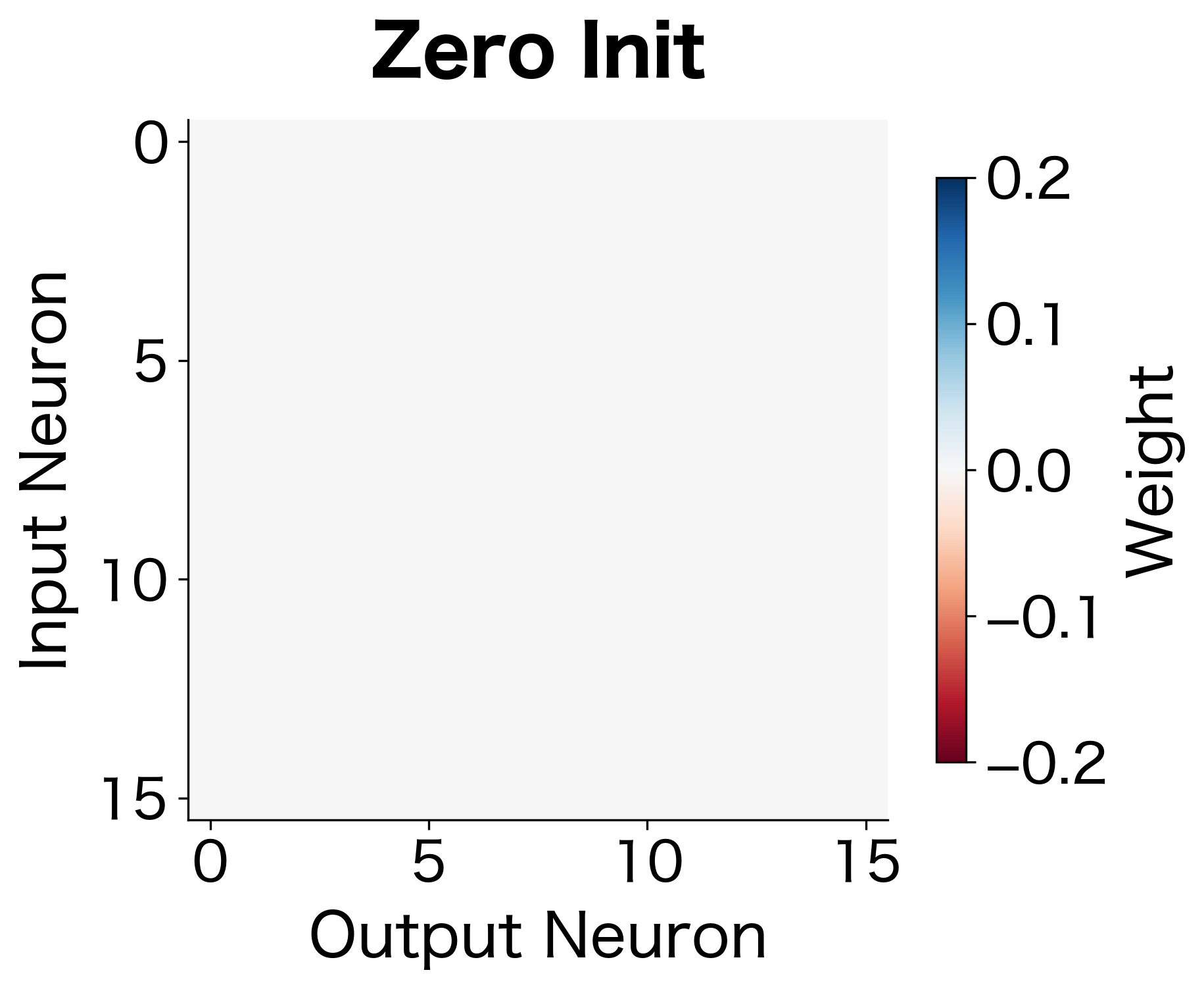
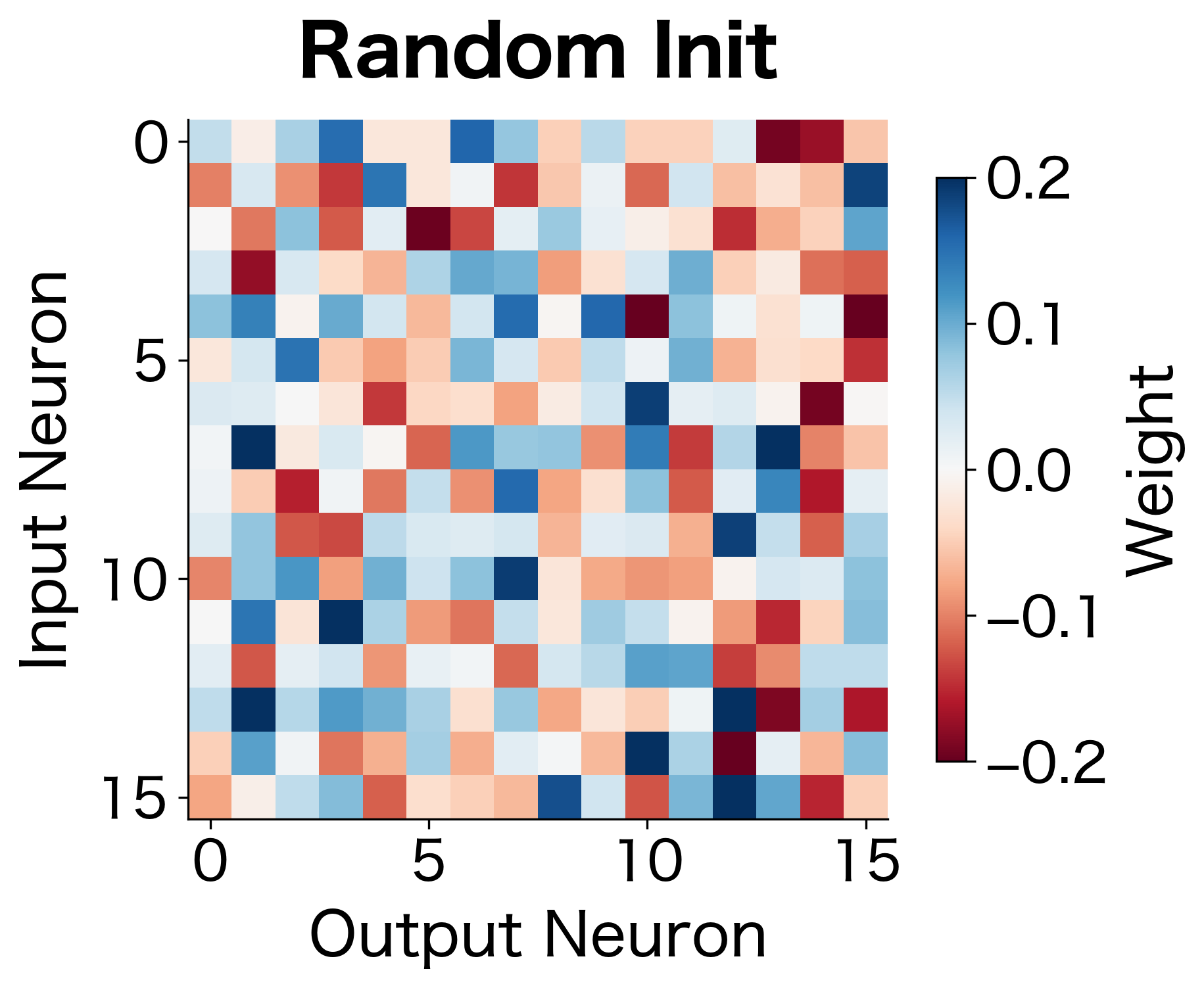
Consider what happens when we initialize all weights to zero. Each neuron in a layer receives the same input and produces the same output. During backpropagation, every neuron receives identical gradients. They all update identically, remaining the same as each other forever. The network has many neurons but effectively behaves as if it has one. This is the symmetry problem: if neurons start identical, they stay identical.
The requirement that neurons in the same layer be initialized differently so they can learn different features. Without symmetry breaking, all neurons compute the same function regardless of network width.
The following visualization contrasts zero initialization (where all weights look identical) with random initialization (where each weight has a distinct value):
We need randomness to break symmetry. But random initialization introduces a new challenge: how do we choose the scale of our random values? Too large, and activations explode. Too small, and gradients vanish.
Let's see this problem in action:
With scale 0.01, activations shrink to nearly zero. With scale 2.0, they saturate at the extremes of tanh (). Neither is good for learning. Scale 0.1 and 1.0 preserve more reasonable activation magnitudes, but which is optimal?
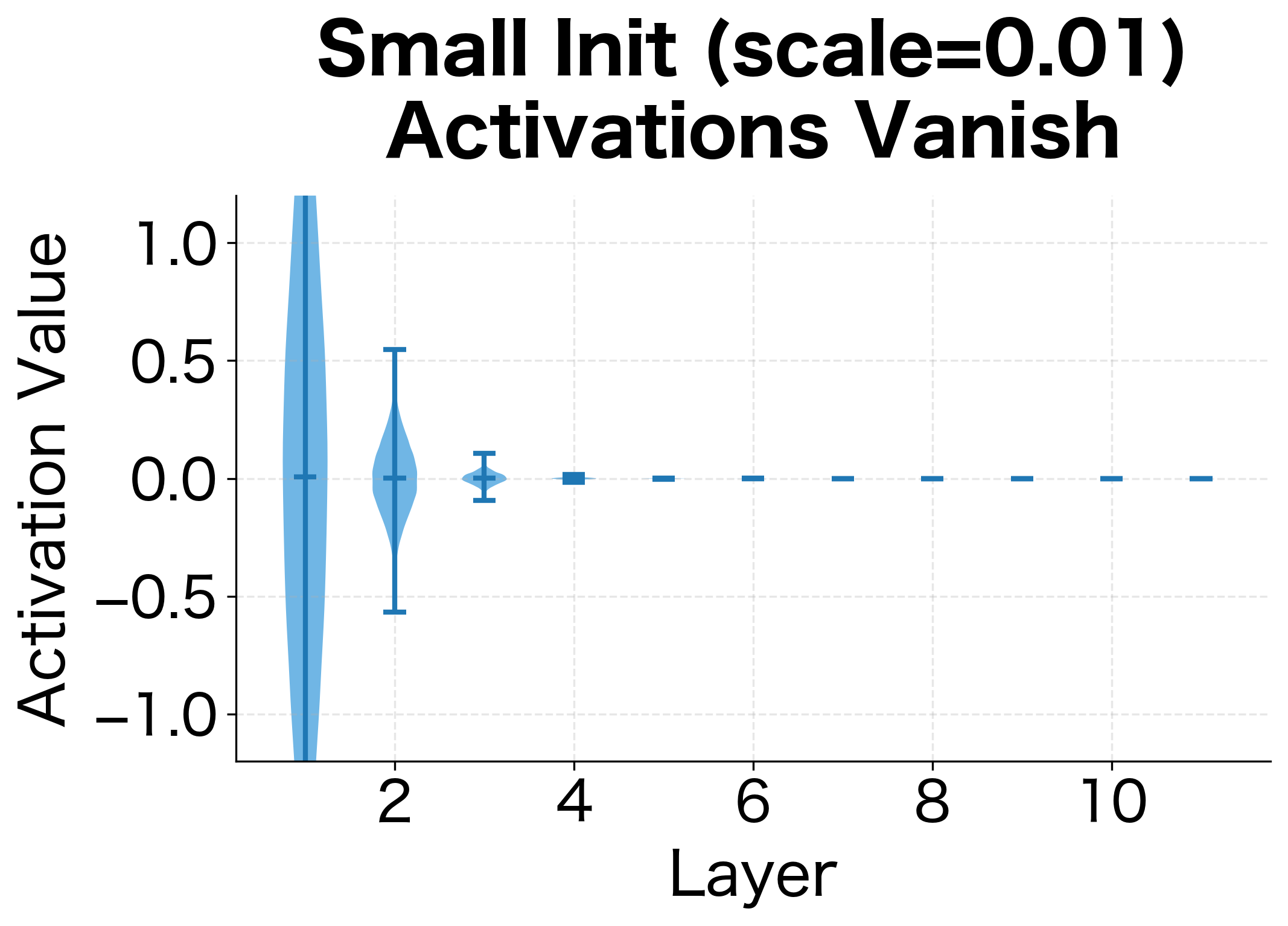
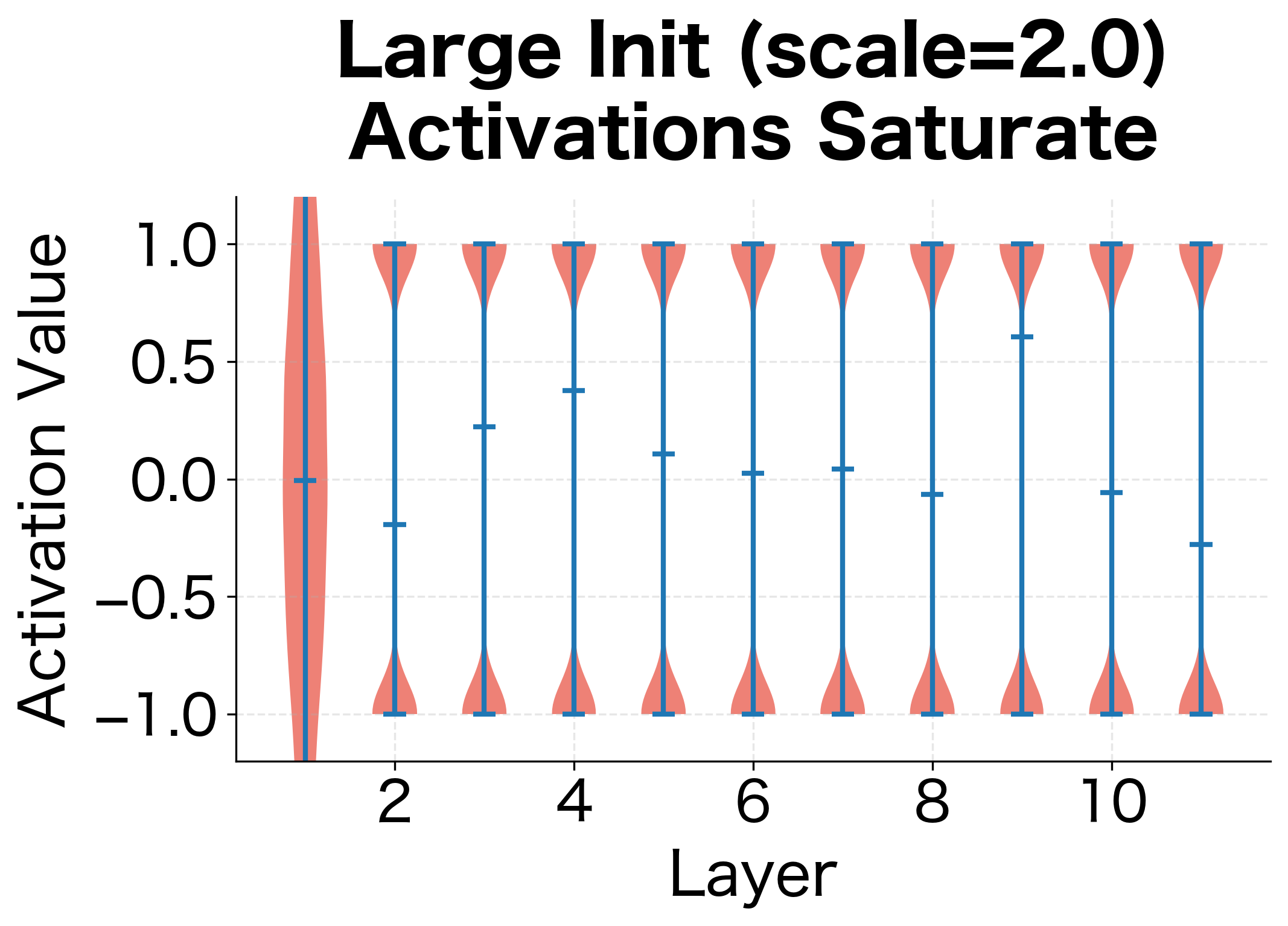
The visualizations reveal two failure modes. With small initialization, activations progressively shrink layer by layer, eventually collapsing to near-zero values. The network loses the ability to distinguish different inputs. With large initialization, activations immediately saturate at the extremes of the activation function. Since the derivative of tanh near is close to zero, gradients vanish here too.
We need an initialization that preserves the variance of activations across layers, keeping them in the useful range where gradients flow effectively.
Variance Analysis of Forward Propagation
The experiments above reveal that initialization scale matters, but they don't tell us what the right scale is. To find it, we need to shift from empirical observation to mathematical analysis. The key question is: how does the variance of activations change as we pass through each layer?
If we can answer this question, we can work backward to determine what weight variance will preserve activation variance across layers. This is the central insight behind principled initialization: treat variance preservation as a design constraint, then solve for the weights that satisfy it.
The Pre-Activation Equation
Consider a single layer with input neurons and output neurons. Each output neuron computes a weighted sum of its inputs before applying the activation function. For a single output neuron, this pre-activation is:
where:
- : the pre-activation value (before applying the activation function)
- : the weight connecting input neuron to this output neuron
- : the activation from input neuron
- : the number of input neurons (fan-in)
This equation is the starting point for our analysis. The pre-activation is a sum of many random terms, and we want to understand how its variance relates to the variances of the weights and inputs.
Deriving the Variance Relationship
Assuming and are independent random variables with zero mean (a reasonable assumption when weights are initialized symmetrically around zero and inputs are centered), we can derive the variance of the pre-activation step by step.
Step 1: Variance of a sum. Since variance is additive for independent random variables:
Step 2: Variance of a product. For two independent, zero-mean random variables and , we have . This follows because and .
Step 3: Combine. Assuming all weights have the same variance and all inputs have variance :
where:
- : variance of the pre-activation output
- : number of input neurons (fan-in)
- : variance of each weight (assumed identical)
- : variance of each input activation (assumed identical)
This result tells us something useful: the output variance equals the input variance multiplied by both the number of inputs and the weight variance. It immediately suggests why naive initialization fails. With 256 input neurons and unit-variance weights, the output variance would be 256 times larger than the input. Each layer amplifies the signal by a factor of , leading to exponential growth.
For a weight matrix connecting two layers, fan-in () is the number of input connections per output neuron, and fan-out () is the number of output connections per input neuron. For a fully connected layer, fan-in equals the input dimension and fan-out equals the output dimension.
Solving for the Optimal Weight Variance
Now we can solve for the weight variance that preserves signal magnitude. To maintain stable variance across layers, we want . Starting from our variance equation:
Setting and dividing both sides by :
Solving for the weight variance:
This is the key insight: the weight variance should scale inversely with the number of input connections. Intuitively, when we sum random terms, the total variance grows proportionally to . To counteract this growth and keep the output variance equal to the input variance, we must shrink each weight's variance by the factor .
Empirical Verification
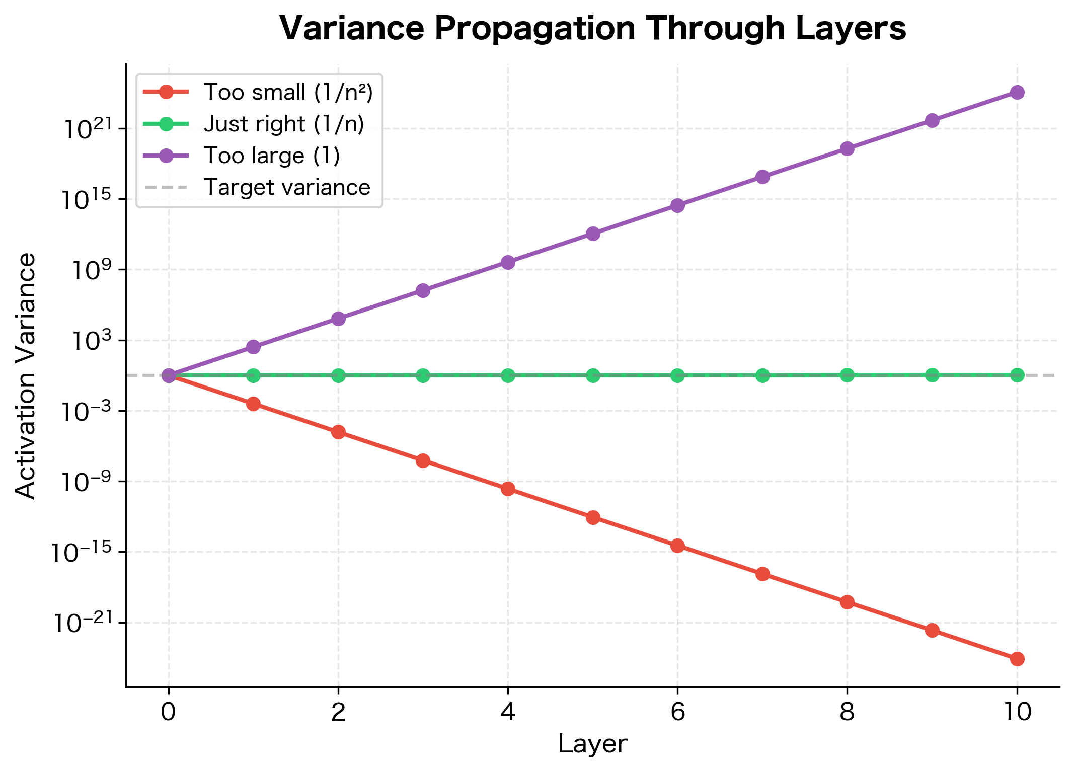
Theory is only useful if it matches reality. Let's verify our analysis by comparing different weight variances and observing how activation variance propagates through a deep network:
With weight variance of , the output variance remains close to the input variance, confirming our analysis. The other choices cause variance to explode or collapse exponentially with depth.
Xavier/Glorot Initialization
Our variance analysis derived the optimal weight variance for the forward pass. But training a neural network involves both forward and backward propagation. Xavier Glorot and Yoshua Bengio, in their influential 2010 paper, recognized that we must consider both directions of signal flow.
Their insight was that gradients during backpropagation face the same variance amplification problem as activations during forward propagation, but in reverse. If we only optimize for forward variance, gradients might explode or vanish. The challenge is finding a weight variance that works reasonably well for both directions.
Forward Pass Requirement
As we derived above, to maintain variance during forward propagation:
where is the fan-in (number of input connections to each neuron).
Backward Pass Requirement
During backpropagation, gradients flow in the opposite direction. Each input neuron receives gradient contributions from all output neurons. By similar reasoning to the forward pass, to maintain gradient variance:
where is the fan-out (number of output neurons that receive input from each input neuron).
The Compromise
We now face a dilemma. The forward pass demands . The backward pass demands . These two requirements conflict unless , which is rare in practice.
Since we cannot satisfy both simultaneously, Glorot and Bengio proposed a compromise that balances both requirements. Rather than favoring one direction over the other, they take the average of the two fan values:
where:
- : the variance of each weight in the layer
- : fan-in (input dimension)
- : fan-out (output dimension)
This is Xavier initialization (also called Glorot initialization). To sample weights from this distribution, we need to convert the variance to distribution parameters.
For a uniform distribution , the variance is . Setting this equal to our target variance:
Solving for :
So we sample:
For a normal distribution , the variance is . Setting this equal to our target variance:
Taking the square root:
So we sample:
A weight initialization scheme where weights are drawn from a distribution with variance . Designed to maintain variance of activations and gradients across layers for networks using tanh or sigmoid activations.
Implementation
With the formulas in hand, implementing Xavier initialization is straightforward. We need to sample weights from a distribution with the correct variance, choosing either uniform or normal based on preference.
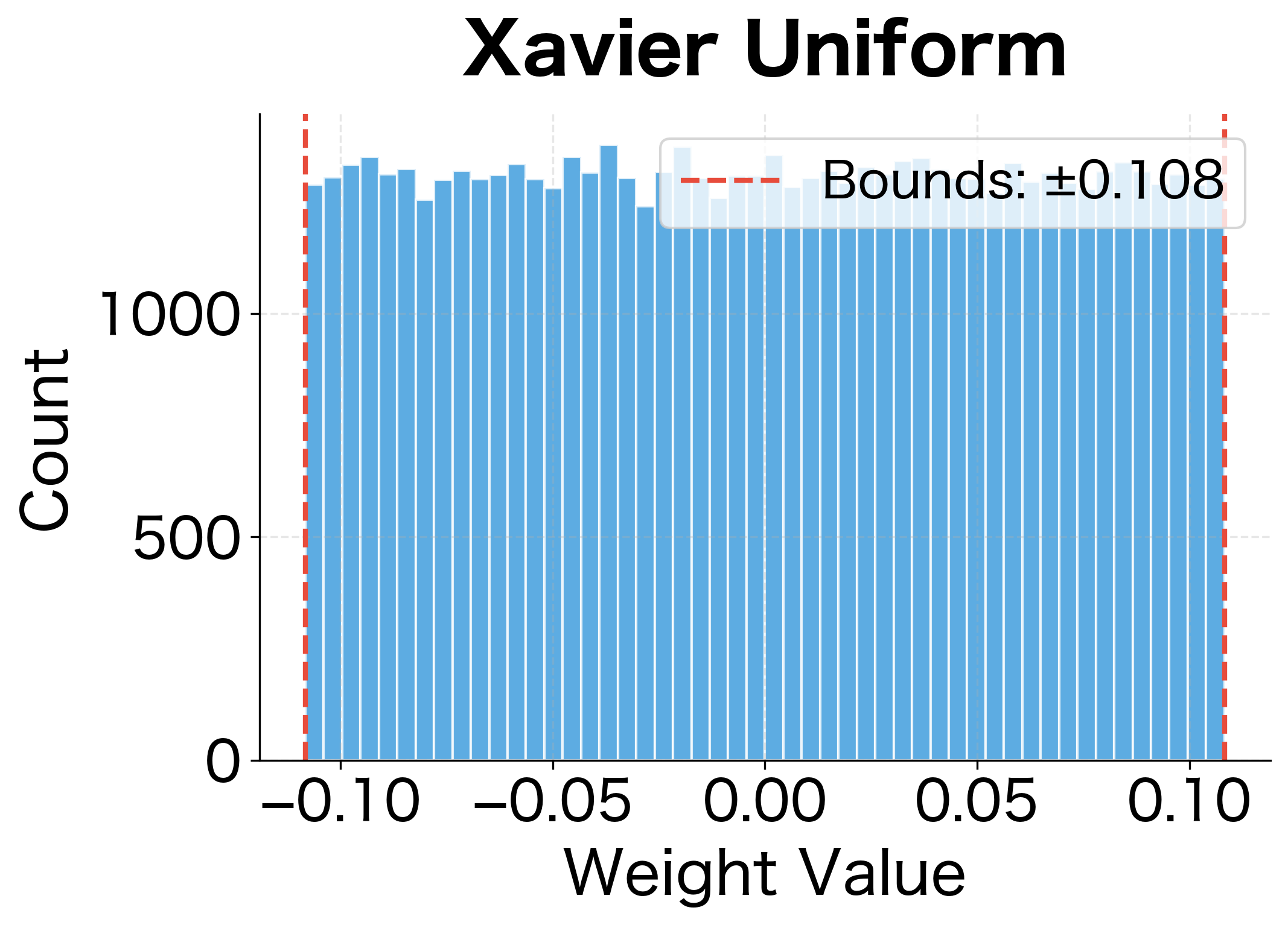
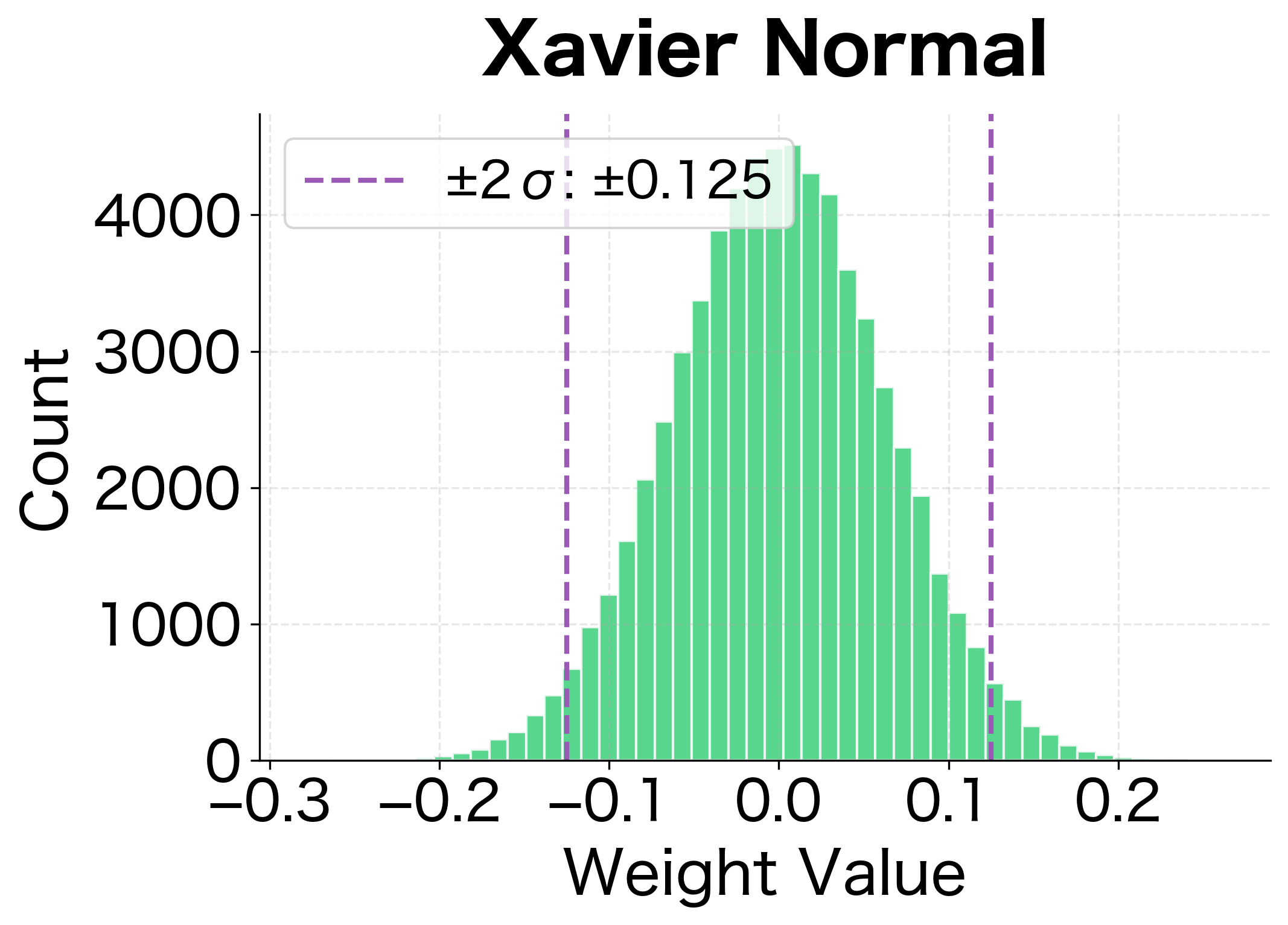
The following visualization shows the resulting weight distributions for both uniform and normal variants:
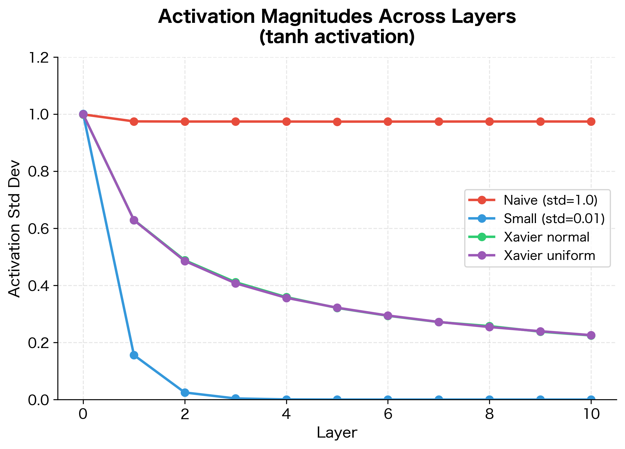
Xavier initialization maintains activation variance much better than naive approaches. The standard deviation stays relatively stable across layers, preventing both vanishing and exploding activations.
He Initialization for ReLU Networks
Xavier initialization was a breakthrough for networks using tanh or sigmoid activations. But by the mid-2010s, ReLU (Rectified Linear Unit) had become the dominant activation function due to its simplicity and effectiveness in avoiding vanishing gradients. Unfortunately, Xavier initialization doesn't work well for ReLU networks.
The problem is that Xavier's derivation assumes the activation function is approximately linear around zero. For tanh and sigmoid, this is reasonable: near zero, they behave almost like the identity function. But ReLU is decidedly non-linear: it sets all negative values to zero, keeping only the positive half of the distribution.
Understanding ReLU's Variance Halving
Consider a pre-activation drawn from a symmetric distribution centered at zero with variance . ReLU sets all negative values to zero while keeping positive values unchanged. Since the distribution is symmetric, approximately half the values are negative, so half become zero.
The variance of the output can be computed as:
For a symmetric zero-mean distribution, the expected value of the positive half is small, and the key term is . Since only positive values contribute, this equals approximately half of :
where:
- : the rectified linear unit function
- : variance of the input pre-activation
This variance halving has severe consequences for deep networks. After layers, the variance becomes approximately , causing activations to shrink exponentially. A 10-layer network would see activations reduced by a factor of . A 20-layer network would see a reduction of over a million.
The following visualization makes this concrete by showing how ReLU transforms a symmetric input distribution:
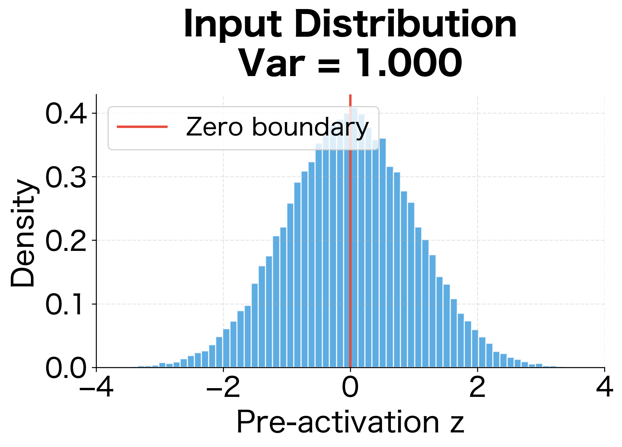
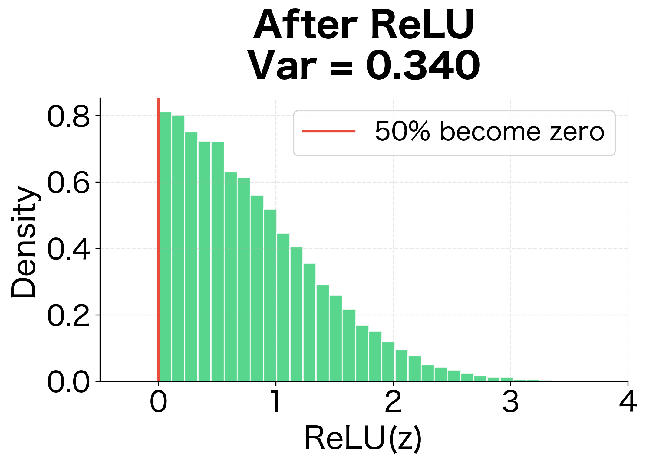
With tanh, Xavier initialization maintains activations reasonably well across 10 layers. With ReLU, however, activations decay dramatically. The decay ratio shows that ReLU activations shrink to a tiny fraction of their initial magnitude, confirming that Xavier is unsuitable for ReLU networks.
Deriving He Initialization
Kaiming He and colleagues addressed this problem in their 2015 paper by modifying the variance analysis to account for ReLU's behavior. The derivation follows the same logic as Xavier, but incorporates the factor of 1/2 from ReLU's variance reduction.
Starting from our original variance equation and incorporating the ReLU effect:
where:
- : variance of the activation output (after ReLU)
- : the variance reduction factor from ReLU
- : fan-in (number of input connections)
- : variance of the weights
- : variance of the input activations
To maintain , we set:
Dividing both sides by and solving for :
This is He initialization (also called Kaiming initialization). The factor of 2 in the numerator compensates exactly for ReLU's variance-halving effect.
A weight initialization scheme where weights are drawn from a distribution with variance . Designed specifically for ReLU networks, accounting for the variance reduction caused by setting negative activations to zero.
Converting Variance to Distribution Parameters
Just as with Xavier, we need to convert our target variance into the parameters of either a normal or uniform distribution.
For a normal distribution, we set the standard deviation to the square root of the target variance:
where denotes a normal distribution with mean and standard deviation .
For a uniform distribution , using the same derivation as Xavier (variance of uniform is ), we solve to get:
Notice that He initialization uses only (fan-in) rather than averaging and like Xavier. This is because He et al. found that matching forward pass variance was more important for training deep ReLU networks. The backward pass still works reasonably well because ReLU's simple gradient (either 0 or 1) doesn't introduce the same variance distortion as its forward computation.
Implementation and Comparison
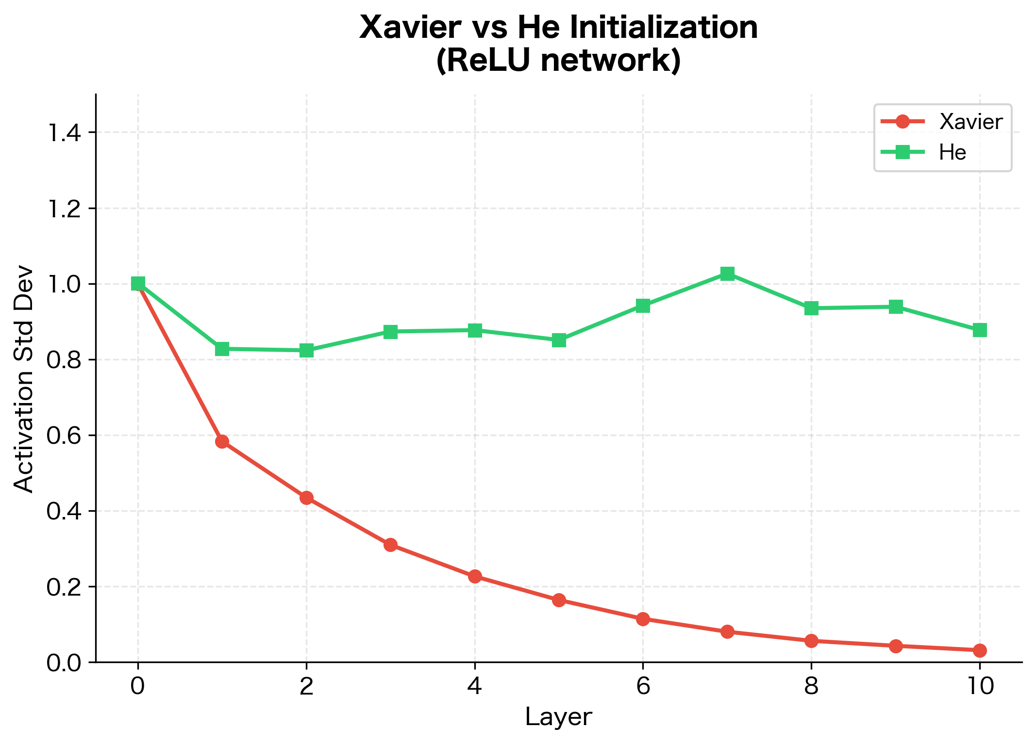
Let's implement He initialization and compare it directly to Xavier on a ReLU network:
He initialization maintains much more stable activation magnitudes in ReLU networks compared to Xavier.
Initialization for Different Activations
We've now seen how Xavier initialization works for symmetric activations and He initialization works for ReLU. But the deep learning toolkit includes many more activation functions, each with its own variance characteristics. The general principle remains the same: analyze how the activation affects variance and adjust the initialization accordingly.
The following table summarizes the recommended initialization for common activations:
| Activation | Recommended Initialization | Weight Variance |
|---|---|---|
| Linear | Xavier | |
| Tanh | Xavier | |
| Sigmoid | Xavier | |
| ReLU | He | |
| Leaky ReLU | He (adjusted) | |
| SELU | LeCun |
The Leaky ReLU Case
For Leaky ReLU with negative slope , the situation is more nuanced than standard ReLU. Instead of zeroing negative inputs, Leaky ReLU scales them by a small factor (typically 0.01 or 0.2). This preserves some information from the negative half of the distribution, meaning the variance reduction is less severe than standard ReLU.
The adjusted variance formula is:
where:
- : the negative slope of Leaky ReLU (typically 0.01 or 0.2)
- : fan-in (number of input connections)
- : a correction factor that accounts for variance from both positive inputs (coefficient 1) and negative inputs (coefficient )
The denominator arises because variance scales with the square of the coefficient. When (standard ReLU), the factor becomes , giving us , which is He initialization. When (linear activation), the factor becomes , giving , which approaches Xavier initialization for the fan-in-only case.
A General Initialization Function
Rather than implementing a separate function for each activation, we can create a unified initialization function that computes the appropriate variance based on the activation type:
The ReLU initialization has the largest standard deviation because it uses the factor of to compensate for variance halving. Tanh uses a gain of approximately 5/3 to account for its non-linearity. SELU uses a standard LeCun initialization with variance , resulting in the smallest standard deviation.
Gradient Analysis
So far, we've focused on how activations propagate forward. But neural network training depends equally on how gradients propagate backward. A good initialization must preserve gradient magnitudes during backpropagation; otherwise, learning signals won't reach the early layers.
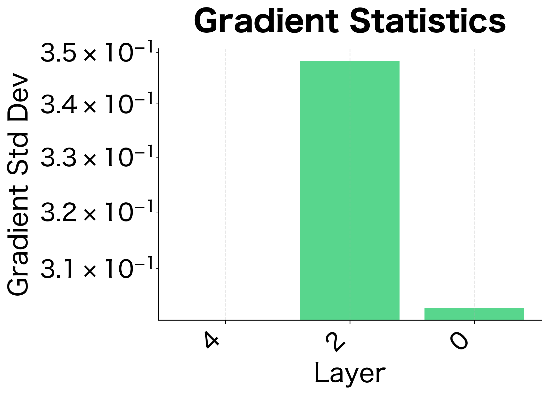
Let's analyze gradient flow and verify that our initializations maintain stable gradients across network depth:
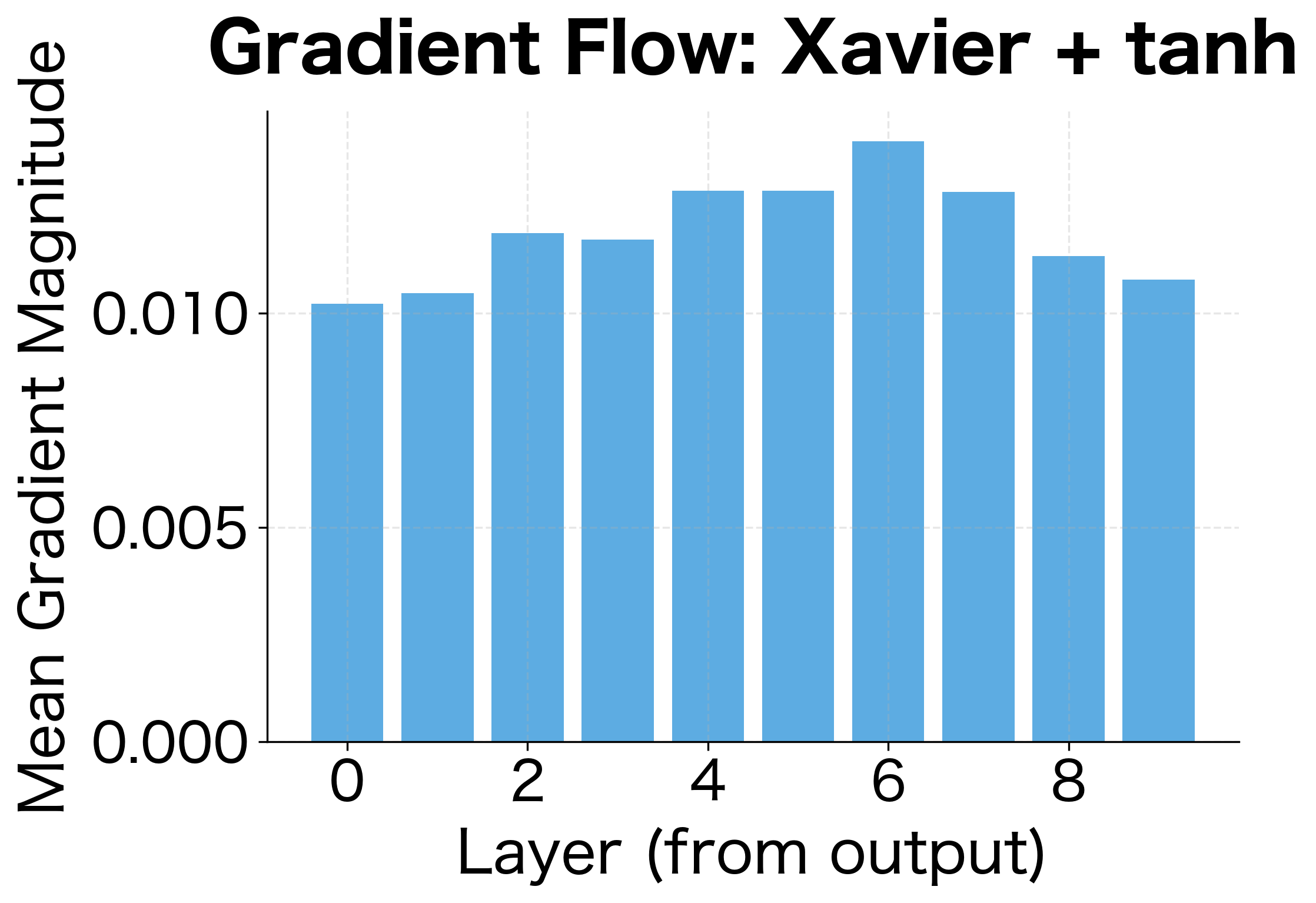
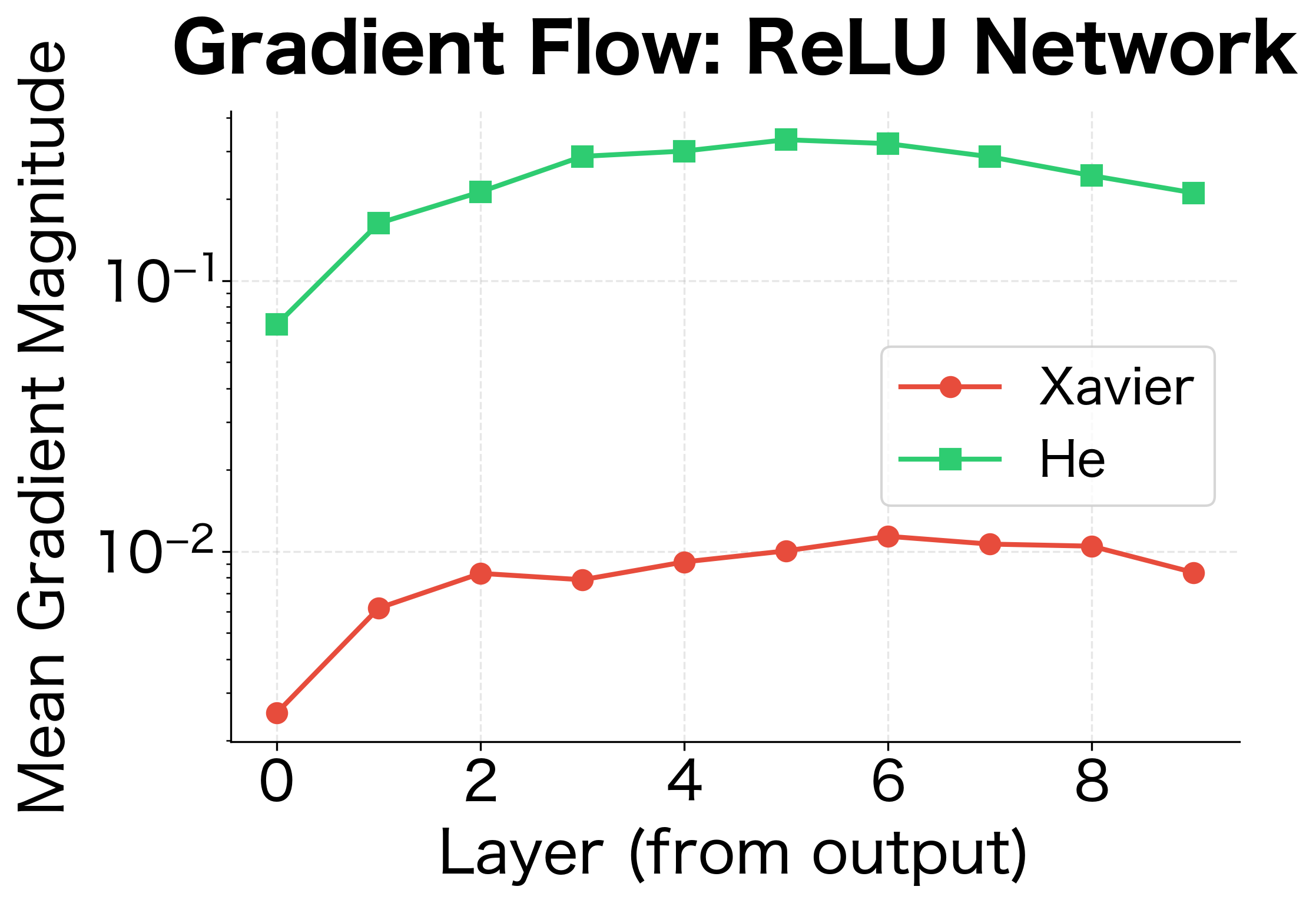
The gradient analysis confirms what we learned from activation analysis: Xavier initialization works well for tanh, maintaining reasonable gradient magnitudes across layers. For ReLU networks, He initialization provides more stable gradient flow.
Practical Implementation with PyTorch
Modern deep learning frameworks provide built-in initialization functions. Let's see how to use PyTorch's initialization utilities:
All initialization methods produce weights centered at zero, as expected. The He methods have slightly larger standard deviations than Xavier because they use only fan-in rather than averaging fan-in and fan-out. The uniform variants show tighter ranges compared to normal variants because the uniform distribution has bounded support.
Training Comparison
Let's compare training dynamics with different initializations on a simple classification task:
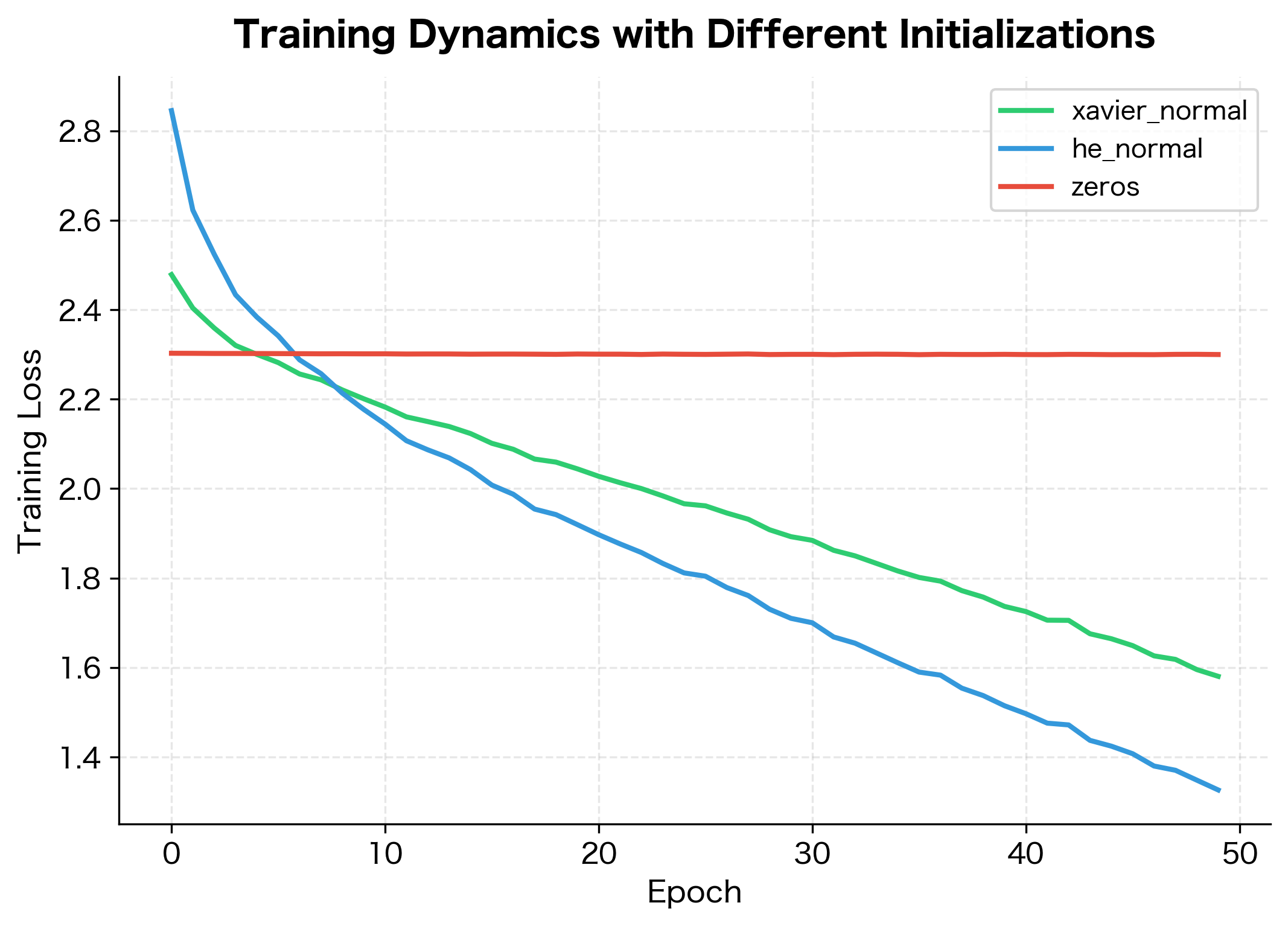
The zero initialization fails to learn at all, stuck at the initial loss. Xavier and He initialization both enable learning, with similar convergence curves for this shallow network. The difference between Xavier and He becomes more pronounced in deeper networks with ReLU activations.
Bias Initialization
While we've focused on weight initialization, biases also need consideration. The common practice is to initialize biases to zero:
Zero biases are almost always a safe choice. Unlike weights, initializing biases to the same value doesn't cause symmetry problems because the gradients for biases depend on the (different) input-weight products.
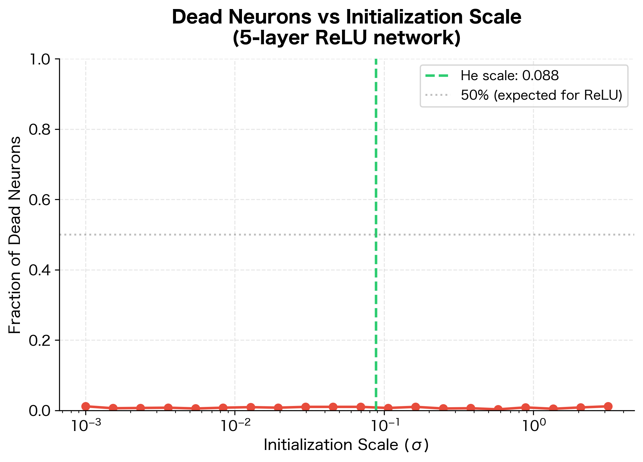
For ReLU networks, some practitioners use small positive biases (like 0.01) to ensure neurons are active initially. This prevents "dead neurons" that never activate because their inputs are always negative. However, modern techniques like batch normalization and careful learning rate scheduling have reduced the importance of this trick.
The following visualization shows how initialization scale affects the fraction of dead neurons in a ReLU network:
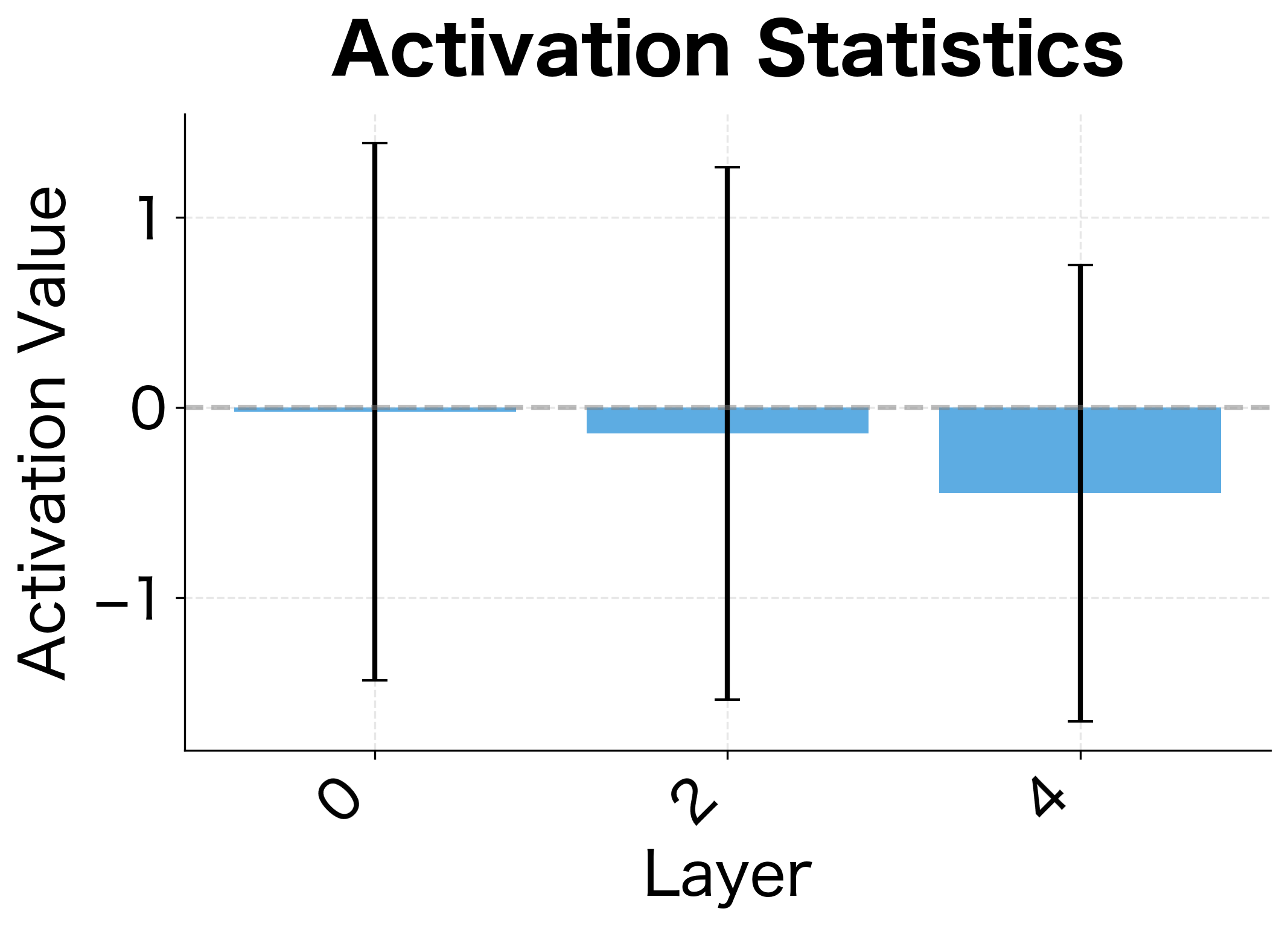
Diagnosing Initialization Problems
When a network fails to train, initialization is a common culprit. Here are diagnostic techniques:
Modern Practices and Alternatives
While Xavier and He initialization remain the defaults, modern deep learning has introduced techniques that reduce sensitivity to initialization:
Batch Normalization
Batch normalization normalizes activations during training, which provides some robustness to initialization:
Layer Normalization
Common in transformers, layer normalization similarly helps with training stability:
Residual Networks
For networks with skip connections, careful initialization of residual branches is important:
The scaling factor (often where is the number of residual blocks) prevents the variance from growing linearly with depth.
Worked Example: Initializing a Language Model
Let's walk through initializing a small transformer-style language model:
The GPT-2 initialization uses a small standard deviation (0.02) for all linear layers. This relatively uniform approach works because layer normalization handles the variance normalization during training.
Limitations and Impact
Weight initialization, while important, is not a magic solution to all training difficulties.
Initialization is just the starting point. A good initialization sets up favorable conditions for learning, but it cannot compensate for basic problems like inappropriate architectures, poor data quality, or incorrect hyperparameters. A network with He initialization will still fail if the learning rate is orders of magnitude too large.
Normalization techniques reduce sensitivity. Batch normalization and layer normalization have reduced the importance of precise initialization. Networks with these components can often train successfully with a wider range of initialization scales. This is one reason modern transformer architectures use a simple standard deviation of 0.02 rather than layer-specific calculations.
Very deep networks remain challenging. For networks with hundreds of layers (like some vision transformers), even careful initialization may not prevent training instabilities. Additional techniques like learning rate warmup, gradient clipping, and careful residual scaling become necessary.
Despite these limitations, understanding initialization principles remains valuable. When a network fails to train, checking initialization is often a productive first step. The mathematical framework we developed, analyzing how variance propagates through layers, provides insight into network behavior that extends beyond just initialization.
Key Parameters
The following parameters control weight initialization behavior in PyTorch:
mode parameter controls fan calculation, while nonlinearitysets the gain factor for the activation function.| Parameter | Values | Effect |
|---|---|---|
mode | 'fan_in', 'fan_out', 'fan_avg' | Determines whether to use input dimensions, output dimensions, or their average for variance calculation. Use fan_in for forward pass stability, fan_out for backward pass stability. |
nonlinearity | 'relu', 'leaky_relu', 'tanh', etc. | Specifies the activation function to compute the appropriate gain factor. Must match the activation used after the layer. |
a (for Leaky ReLU) | 0.01 (default), 0.2, etc. | The negative slope parameter for Leaky ReLU. Affects the variance correction factor . |
For nn.init.kaiming_normal_ and nn.init.kaiming_uniform_:
- Use
mode='fan_in'(default) to preserve forward pass variance - Use
mode='fan_out'to preserve backward pass variance - Set
nonlinearity='relu'for standard ReLU or specify'leaky_relu'with theaparameter
For nn.init.xavier_normal_ and nn.init.xavier_uniform_:
- These use
fan_avgmode internally (no mode parameter) - The
gainparameter multiplies the standard deviation (default 1.0) - Use
gain=nn.init.calculate_gain('tanh')for tanh activations
Summary
Weight initialization determines whether a neural network can learn effectively from the start. The core principle is variance preservation: weights should be scaled so that activations and gradients maintain reasonable magnitudes as they propagate through layers.
Key takeaways:
- Zero initialization causes symmetry: All neurons learn the same thing, wasting network capacity
- Xavier initialization uses variance , designed for tanh and sigmoid activations
- He initialization uses variance , accounting for ReLU's variance-halving effect
- Biases are typically initialized to zero, which doesn't cause symmetry problems
- Modern architectures with batch or layer normalization are more robust to initialization, but still benefit from reasonable starting values
- Diagnostic tools can identify initialization problems by examining activation and gradient statistics
The next chapter covers batch normalization, a technique that normalizes activations during training and further reduces sensitivity to initialization while enabling training of even deeper networks.
Quiz
Ready to test your understanding? Take this quick quiz to reinforce what you've learned about weight initialization in neural networks.

Comments