Full Fine-tuning: Hyperparameters & Learning Rate Schedules

In the previous chapter, we established that transfer learning enables us to leverage knowledge from pre-trained models, rather than training from scratch. Full fine-tuning is the most direct approach to transfer learning. We take a pre-trained model, update all of its parameters on task-specific data, and produce a specialized model. This chapter covers the mechanics of full fine-tuning, including the hyperparameters that govern the process and the subtle decisions that determine success or failure. We'll explore each step in detail, explain why each choice matters, and provide practical guidance for configuring your own fine-tuning runs.

Full fine-tuning updates every parameter in the model during training on your downstream task. For a model like BERT-base with 110 million parameters, this means computing gradients for and updating all 110 million weights. This approach maximizes the model's capacity to adapt to new tasks, but it requires significant computational and memory resources. Understanding how to configure the fine-tuning process correctly is essential for achieving good results.

Full fine-tuning follows a structured procedure that transforms a general-purpose pre-trained model into a task-specific one. While conceptually simple, each step involves decisions that affect the final model's performance, representing a careful balance between preserving pre-trained knowledge and adapting the model to excel at a specific downstream task.

The process begins by loading a pre-trained checkpoint. This checkpoint contains the learned weights from pre-training on large corpora. For encoder models like BERT, these weights encode rich contextual representations that capture the nuances of language (syntax, semantics, and even some world knowledge). For decoder models like GPT, they capture language generation capabilities that enable fluent text production. The checkpoint represents months of compute time and billions of training examples. All of this is distilled into a set of parameter values that serve as our starting point.

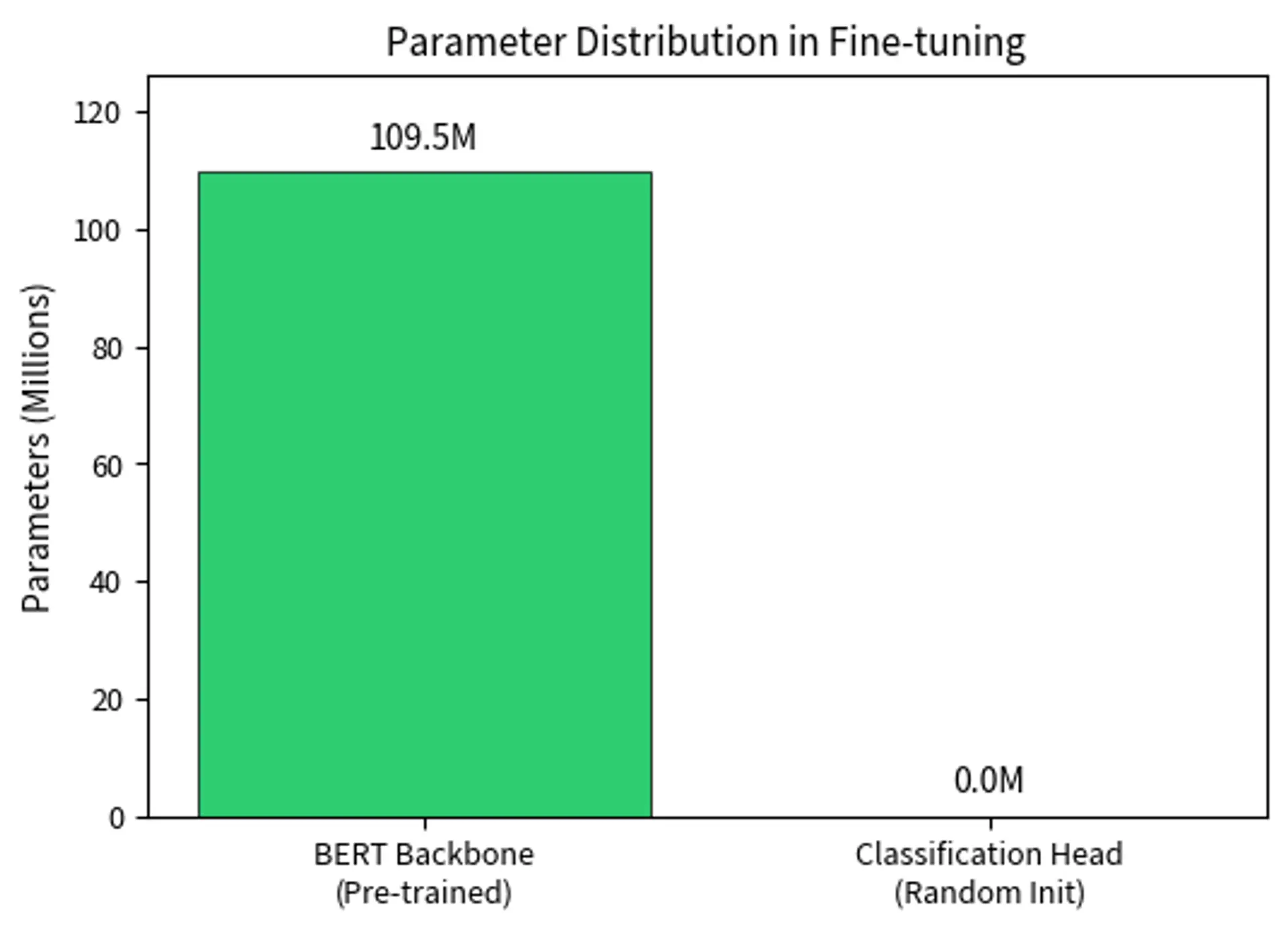
The model contains over 100 million parameters, all of which are trainable. With all parameters trainable, every weight in both the BERT backbone and the classification head receives gradient updates during fine-tuning, allowing maximum adaptation to the task while requiring significant computational resources. The equality between total and trainable parameters distinguishes full fine-tuning from parameter-efficient methods, where only a subset of parameters receive updates.

The key parameters for loading the model are:

• model_name: The identifier for the pre-trained model on Hugging Face Hub.
• num_labels: Number of output classes for the classification task.

When loading a model for a downstream task, the library adds a task-specific head on top of the pre-trained backbone. This head converts the model's internal representations into task-specific outputs, such as class probabilities for classification. For sequence classification, this is typically a linear layer that maps the final hidden states to class logits. The architecture follows a simple principle. The pre-trained model produces rich, contextual representations, and the task head transforms these representations into the specific format required by your task.

Key concepts:

• task-specific head: a small neural network layer added on top of the pre-trained model to produce outputs for the target task
• final hidden states: the contextual representations produced by the pre-trained backbone for each token
• class logits: unnormalized scores for each class that will be converted to probabilities via softmax

The task-specific head acts as a bridge between the model's rich internal representations and the specific output format required by the task. For classification, it reduces the high-dimensional hidden states to a simple score per class. This reduction is mathematically straightforward: a linear transformation projects from the hidden dimension (768 for BERT-base) to the number of classes (2 for binary classification), but the simplicity of this mapping belies the complexity of the representations it receives.

The backbone parameters are initialized from pre-training, while the classification head is randomly initialized. This asymmetry has important implications for training. The backbone starts with excellent representations, while the head must learn from scratch to interpret them correctly.

Fine-tuning requires task-specific labeled data. The data must be tokenized using the same tokenizer that was used during pre-training to ensure consistency in how text is represented. This consistency is crucial because the model learned to interpret specific token patterns during pre-training, and using a different tokenization scheme would create a mismatch between the input format and the model's learned expectations.

The Rotten Tomatoes dataset provides thousands of movie reviews split across training, validation, and test sets. The training set size determines how many parameter updates will occur per epoch, while the validation and test sets allow us to monitor generalization and measure final performance on unseen data. The tokenization process converts text into the input format expected by the model. This format includes input IDs, attention masks, and optionally token type IDs. Using max_length=128 truncates longer sequences and pads shorter ones to a fixed length. This enables efficient batched processing.

The key parameters for dataset preparation are:

• padding: Strategy for padding sequences. "max_length" pads all sequences to a fixed length.
• truncation: Whether to truncate sequences longer than max_length.
• max_length: Maximum sequence length, chosen to balance computational efficiency with information retention

Key tokenization concepts:

• input IDs: integer tokens representing each word or subword piece in the vocabulary, mapping text to the numerical format required by the model
• attention masks: binary values indicating which tokens are real content (1) versus padding (0), ensuring the model ignores padding when computing attention
• token type IDs: optional integers distinguishing different segments in paired-sequence tasks, such as separating question from context

The attention mask is crucial because it prevents padded positions from influencing the model's computations, ensuring that only meaningful content contributes to the final representations. Without this mechanism, padding tokens would distort the attention patterns and corrupt the contextual representations that make transformers so effective.

Fine-tuning hyperparameters differ substantially from pre-training settings. Pre-training uses large batch sizes, high learning rates, and millions of steps. Fine-tuning uses smaller batch sizes, much lower learning rates, and only a few epochs. This approach prevents the pre-trained knowledge from being overwritten too quickly, preserving the model's existing capabilities while allowing task-specific adaptation. The philosophy underlying these choices reflects a fundamental insight: we are not learning from scratch, but rather making targeted adjustments to an already capable model.

These settings represent a reasonable starting point for fine-tuning BERT on a classification task. The learning rate of $2 \times 10^{-5}$ is roughly 100 times smaller than typical pre-training learning rates. The warmup ratio of 0.1 means the learning rate will increase linearly for the first 10% of training steps before following the decay schedule. Each of these choices reflects accumulated wisdom from thousands of fine-tuning experiments across the research community.

With the model, data, and configuration in place, training proceeds through the standard optimization loop. The Trainer API handles batching, gradient computation, parameter updates, and evaluation. Behind this convenient abstraction lies a sophisticated process that coordinates data loading, forward passes through the model, loss computation, backward passes for gradient calculation, and parameter updates according to the optimizer's rules.

The final training loss indicates successful convergence. This decreasing loss shows that the model has adapted its representations to the sentiment classification task, with both the pre-trained backbone and classification head updating to minimize prediction errors on movie reviews. During training, all parameters receive gradient updates. The pre-trained backbone parameters are nudged toward representations that better serve the classification task, while the randomly initialized classification head learns to map these representations to class predictions. The interplay between backbone adaptation and head learning creates a collaborative optimization process where both components adjust to work together effectively.

Fine-tuning success depends on correctly setting several interconnected hyperparameters. Unlike pre-training, where massive compute budgets allow for extensive hyperparameter searches, fine-tuning often requires getting these settings right with limited experimentation. Understanding the principles behind each hyperparameter helps practitioners make informed choices rather than relying solely on trial and error.

The learning rate is the most critical hyperparameter in fine-tuning. It controls how much the weights change in response to computed gradients. A learning rate that's too high will destroy pre-trained representations, causing the model to forget what it learned during pre-training. A learning rate that's too low will result in insufficient adaptation to the new task. Finding the right balance requires understanding the unique constraints of fine-tuning compared to training from scratch.

For transformer models, fine-tuning learning rates typically fall in the range:

where:

• $\text{lr}_{\text{fine-tune}}$: the learning rate used during fine-tuning
• The range $[10^{-5}, 5 \times 10^{-5}]$: typical values that balance adaptation speed with preservation of pre-trained knowledge. The lower bound $10^{-5}$ represents the minimum learning rate that still allows meaningful adaptation, and the upper bound $5 \times 10^{-5}$ represents the maximum rate before risking destruction of pre-trained representations

This narrow range reflects a fundamental trade-off. Rates that are too high destroy pre-trained representations, while rates that are too low fail to adapt the model to new task patterns. The exponential notation ($10^{-5}$ means 0.00001) emphasizes how dramatically these rates differ from standard neural network training, where learning rates of 0.001 to 0.1 are common. The difference spans two to four orders of magnitude, underscoring that fine-tuning operates in a fundamentally different regime than training from random initialization.

The intuition behind this narrow range is that pre-trained models have already learned useful representations. We want to gently nudge these representations toward our specific task, not overwrite them entirely. Think of fine-tuning like adjusting a musical instrument. A violin that's slightly out of tune needs small, careful adjustments. Large, aggressive changes would destroy its calibration entirely. Similarly, a pre-trained model has found a good region of parameter space, and we want to explore nearby configurations rather than jumping to distant, potentially inferior locations. The mathematical relationship can be expressed as follows:

where:

• $\text{lr}_{\text{pre-train}}$: learning rate during pre-training (typically $1 \times 10^{-4}$ to $1 \times 10^{-3}$)
• $\text{lr}_{\text{fine-tune}}$: learning rate during fine-tuning (typically $1 \times 10^{-5}$ to $5 \times 10^{-5}$)
• $k$: the reduction factor, typically ranging from 10 to 100, representing how much we scale down the pre-training rate
• The division by $k$: scales down the pre-training rate to preserve learned representations while still allowing adaptation
• The approximation symbol $\approx$: acknowledges that this is a practical guideline rather than an exact formula, since optimal rates vary by task and dataset

This relationship captures the core principle of fine-tuning: we start from good parameters and make small adjustments. The reduction factor $k$ quantifies "how small" those adjustments should be, balancing preservation of pre-trained knowledge versus adaptation to the new task. The formula provides a principled way to derive a starting learning rate when you know the pre-training configuration, and it explains why fine-tuning rates fall into such a specific, narrow range.

The reduction factor $k$ encodes our empirical understanding that pre-trained models need gentler updates than randomly initialized networks. When $k=10$, a pre-training rate of $1 \times 10^{-4}$ becomes a fine-tuning rate of $1 \times 10^{-5}$. When $k=100$, a pre-training rate of $1 \times 10^{-3}$ becomes a fine-tuning rate of $1 \times 10^{-5}$. Both scenarios arrive at similar fine-tuning rates despite different pre-training configurations, suggesting convergence toward an optimal fine-tuning regime.

The reduction factor $k$ typically ranges from 10 to 100. Fine-tuning learning rates are one to two orders of magnitude smaller than pre-training rates. This dramatic reduction is necessary because pre-trained parameters have already converged to representations that capture general linguistic knowledge. These representations are not perfect for any specific task, but they provide an excellent foundation. Large updates would destroy this foundation, requiring the model to rebuild representations it already possesses.

Fine-tuning typically requires only 2-5 epochs over the training data. This stands in stark contrast to training from scratch, which might require hundreds of epochs. The pre-trained model starts from an excellent initialization, so it needs only minor adjustments to perform well on the new task. The model has already learned how to process language. It just needs to learn how to apply that knowledge to your specific problem.

Training for too many epochs leads to overfitting, where the model memorizes the training data rather than learning generalizable patterns. Because fine-tuning datasets are typically much smaller than pre-training corpora, this risk is particularly acute. A pre-training corpus might contain billions of tokens, while a fine-tuning dataset might contain only thousands or tens of thousands of examples. This size disparity means the model can easily memorize the fine-tuning data, losing its ability to generalize.

Batch size affects both training dynamics and computational requirements. Larger batches provide more stable gradient estimates. However, they require more memory. In fine-tuning, common batch sizes range from 16 to 32 for models like BERT on consumer GPUs. These moderate batch sizes balance the need for reliable gradient estimates against memory constraints and training speed.

The interaction between batch size and learning rate is important: larger batches generally benefit from higher learning rates, a relationship known as the linear scaling rule. If you double the batch size, you can approximately double the learning rate to maintain similar training dynamics. This relationship arises because larger batches produce more stable gradient estimates, allowing the optimizer to take larger steps without risking divergence.

Warmup gradually increases the learning rate from zero to its target value over the first portion of training. This prevents the randomly initialized classification head from causing large, destabilizing gradient updates at the start of training. The newly added classification head produces essentially random outputs initially, leading to large loss values and correspondingly large gradients. If applied at the full learning rate, these gradients could corrupt the carefully learned backbone representations.

A typical warmup ratio is 0.06 to 0.1, meaning the learning rate ramps up linearly for the first 6-10% of total training steps. This gradual increase gives the classification head time to develop basic competence. Then the full learning rate is applied to the backbone. The warmup schedule can be expressed mathematically as follows:

where:

• $\text{lr}(t)$: the learning rate at training step $t$
• $\text{lr}_{\text{max}}$: the target maximum learning rate (e.g., $2 \times 10^{-5}$)
• $t$: the current training step
• $T_{\text{warmup}}$: the number of warmup steps
• The ratio $\frac{t}{T_{\text{warmup}}}$: the linear interpolation factor, starting at 0 and reaching 1 at the end of warmup

This piecewise function defines two phases: (1) during warmup ($t < T_{\text{warmup}}$), the learning rate increases linearly from 0 to $\text{lr}_{\text{max}}$, and (2) after warmup ($t \geq T_{\text{warmup}}$), the learning rate stays constant at $\text{lr}_{\text{max}}$ (or begins following a decay schedule, if configured). The piecewise structure reflects the distinct needs of early versus later training. Caution is needed initially, then full engagement follows once the model has stabilized.

The function ensures a smooth ramp-up. At $t = 0$:

At $t = T_{\text{warmup}}$:

The linear interpolation prevents sudden jumps in the learning rate, which is critical because the randomly initialized classification head produces large, unstable gradients at the start of training. By ramping up gradually, we give the head time to learn reasonable outputs before applying full learning rate updates to the pre-trained backbone. The head moves from random predictions toward sensible outputs over the warmup period, and by the time the full learning rate engages, its gradients reflect meaningful learning signals rather than noise from random initialization.

Why warmup matters: Without this gradual ramp-up, the random classification head would compute meaningless losses on the first few batches, generating enormous gradients that could corrupt the carefully pre-trained backbone weights. Warmup gives the head several hundred steps to develop basic competence before we fully engage the learning rate. The technique transforms what could be a destructive start into a controlled initialization process.

Without warmup, the initial gradient updates (driven partly by the untrained classification head) can corrupt the pre-trained representations before they have a chance to adapt.

Weight decay (L2 regularization) prevents parameters from growing too large and encourages simpler models. For fine-tuning, values around 0.01 are common. As we discussed in the AdamW chapter, decoupled weight decay handles this more correctly than traditional L2 regularization in adaptive optimizers.

Choosing the right learning rate requires balancing competing concerns. We want enough change to adapt to the new task, but not so much that we destroy pre-trained knowledge. This balancing act is at the heart of successful fine-tuning. Understanding the tools available helps practitioners navigate this challenge effectively.

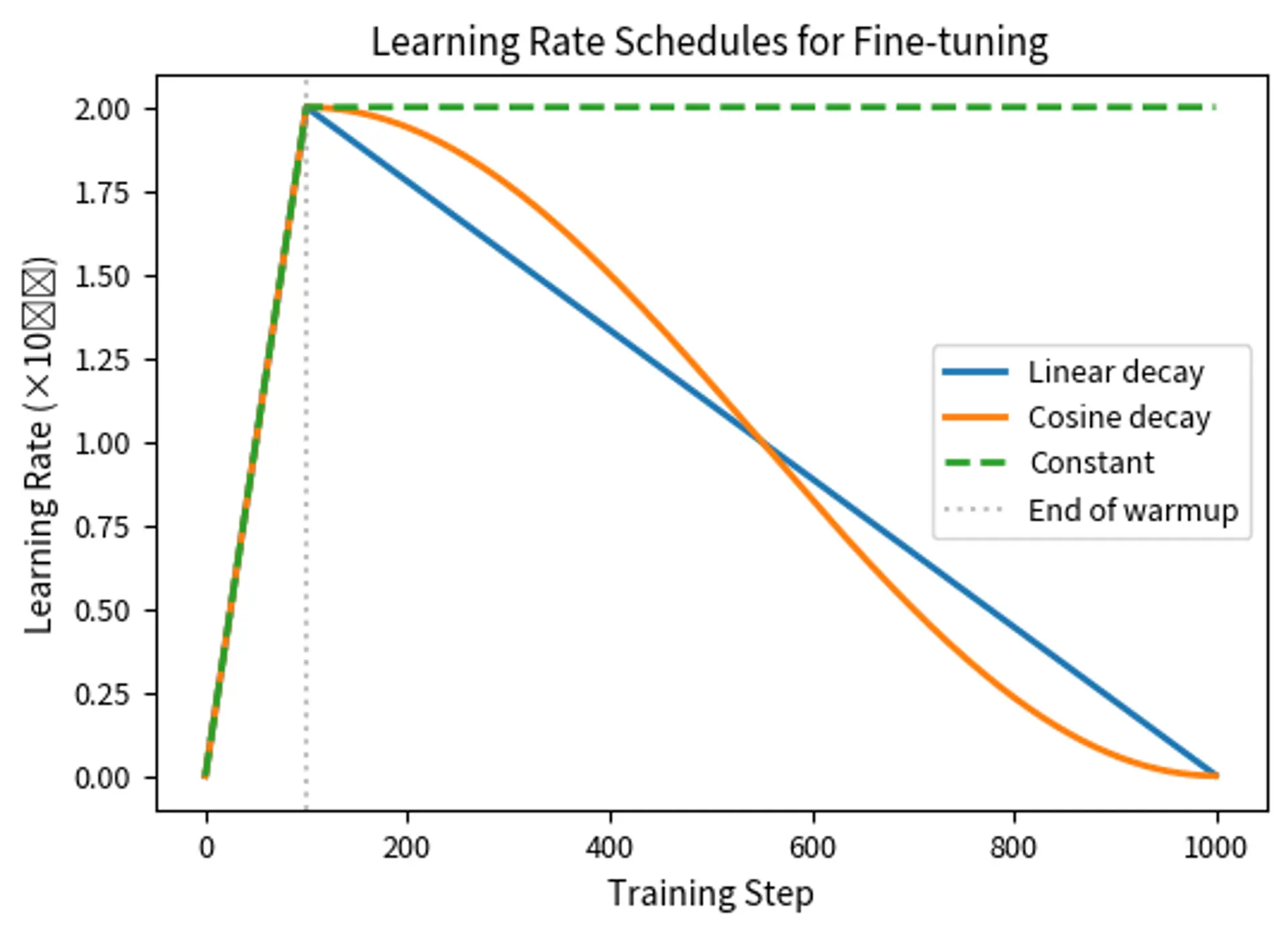
The learning rate typically follows a schedule that varies it throughout training. The most common schedules for fine-tuning are designed to start with more aggressive learning (once warmup completes) and gradually become more conservative as training progresses. This pattern reflects the intuition that early training benefits from larger updates to establish good task-specific representations, while later training benefits from smaller updates to fine-tune details without overshooting optimal values.

Linear decay starts at the target learning rate after warmup and decreases linearly to zero by the end of training. This straightforward approach provides a predictable reduction in learning rate that many practitioners find effective. After the warmup phase, the schedule follows:

where:

• $\text{lr}(t)$: the learning rate at training step $t$ (after warmup)
• $\text{lr}_{\text{max}}$: the maximum learning rate reached after warmup
• $t$: the current training step (where $t \geq T_{\text{warmup}}$)
• $T_{\text{warmup}}$: the number of warmup steps
• $T_{\text{total}}$: the total number of training steps
• The term $(1 - \frac{t - T_{\text{warmup}}}{T_{\text{total}} - T_{\text{warmup}}})$: the linear decay factor, starting at 1 and reaching 0 at the end of training
• The numerator $t - T_{\text{warmup}}$: measures how many steps have elapsed since warmup ended
• The denominator $T_{\text{total}} - T_{\text{warmup}}$: measures the total number of training steps after warmup
• Their ratio: represents the fraction of post-warmup training completed, growing from 0 to 1

To understand how this formula works, let's examine the decay factor at key points during training. This analysis reveals how the schedule transitions smoothly from full learning rate to zero.

At the start of decay ($t = T_{\text{warmup}}$):

This gives the full learning rate: $\text{lr}(T_{\text{warmup}}) = \text{lr}_{\text{max}} \times 1 = \text{lr}_{\text{max}}$.

At the end of training ($t = T_{\text{total}}$):

This reduces the learning rate to zero: $\text{lr}(T_{\text{total}}) = \text{lr}_{\text{max}} \times 0 = 0$.

The intuition is that as we approach the end of training, we want smaller updates to avoid overshooting the optimal parameters. At intermediate points, the decay factor falls between 0 and 1, creating a smooth linear transition from the maximum learning rate to zero. Starting with larger updates allows faster initial progress, while ending with tiny updates enables fine refinement. This linear decrease provides a gentle transition that helps the model converge smoothly, making it the default choice for BERT-style fine-tuning because it works well across many tasks. The simplicity of linear decay also makes it easy to reason about: halfway through training, the learning rate will be at half its maximum value.

Cosine decay decreases the learning rate following a cosine curve with a smoother transition. It decreases slowly at first, more rapidly in the middle, and slowly again at the end. This shape reflects the mathematical properties of the cosine function and provides a more gradual transition than linear decay. After warmup, the schedule follows:

where:

• $\text{lr}(t)$: the learning rate at training step $t$ (after warmup)
• $\text{lr}_{\text{max}}$: the maximum learning rate reached after warmup
• $t$: the current training step (where $t \geq T_{\text{warmup}}$)
• $T_{\text{warmup}}$: the number of warmup steps
• $T_{\text{total}}$: the total number of training steps
• $\cos(\cdot)$: the cosine function, which oscillates between -1 and 1, creating the smooth decay curve when combined with the other terms
• The argument $\pi \times \frac{t - T_{\text{warmup}}}{T_{\text{total}} - T_{\text{warmup}}}$: maps training progress linearly from 0 to $\pi$
• The cosine of this argument: decreases from $\cos(0) = 1$ to $\cos(\pi) = -1$ as training progresses
• The addition of 1: shifts the range from [-1, 1] to [0, 2]
• The factor 0.5: scales the range from [0, 2] to [0, 1], giving the final decay multiplier

Let's verify the formula at key points to confirm it behaves as expected. Understanding these boundary conditions helps build intuition for how the schedule operates throughout training.

At the start of decay ($t = T_{\text{warmup}}$):

\begin{aligned} \text{lr}(T_{\text{total}}) &= \text{lr}{\text{max}} \times 0.5 \times \left(1 + \cos\left(\pi \times \frac{T{\text{total}} - T_{\text{warmup}}}{T_{\text{total}} - T_{\text{warmup}}}\right)\right) && \text{(substitute } t = T_{\text{total}} \text{)} \ &= \text{lr}{\text{max}} \times 0.5 \times (1 + \cos(\pi)) && \text{(simplify argument)} \ &= \text{lr}{\text{max}} \times 0.5 \times (1 + (-1)) && \text{(evaluate } \cos(\pi) = -1 \text{)} \ &= 0 && \text{(compute)} \end{aligned}

While default values like $2 \times 10^{-5}$ work well for many BERT fine-tuning scenarios, optimal learning rates vary by model, task, and dataset size. Several strategies can help identify good values, each offering different trade-offs between thoroughness and computational cost.

Grid search evaluates a small set of candidate learning rates, typically varying by factors of 2-3 (e.g., 1e-5, 2e-5, 5e-5). With small fine-tuning datasets, this remains computationally feasible. The approach is systematic and provides clear comparisons across candidates.

Learning rate finder gradually increases the learning rate during a short training run, plotting loss against learning rate. The optimal learning rate is often just before the loss begins to increase sharply. This technique provides quick insights without full training runs. The method exploits the fact that loss should decrease as learning rate increases from very small values, but will eventually start increasing when the learning rate becomes too large.

Model-specific heuristics leverage community knowledge. BERT models typically work well with 2e-5 to 3e-5. Larger models like RoBERTa-large often benefit from slightly lower rates. GPT-style decoder models may need different ranges depending on the task. These heuristics encode the collective experience of thousands of practitioners and provide reliable starting points.

Batch size interacts with training in multiple ways, affecting memory usage, gradient quality, and convergence behavior. Understanding these interactions helps practitioners make informed choices when configuring their training runs.

The primary constraint on batch size is GPU memory. Each sample in a batch requires memory for:

• Input tensors (token IDs, attention masks)
• Intermediate activations (stored for backward pass)
• Gradients for all parameters
• Optimizer states (momentum buffers for Adam)

For a model like BERT-base with sequences of length 512, batch sizes of 8-16 are common on consumer GPUs with 12-16GB of memory. These memory requirements accumulate across all samples in the batch, creating a direct relationship between batch size and peak memory usage.

The memory requirements break down into several components:

• Input tensors: the tokenized representation of each text sample, including token IDs and attention masks
• Intermediate activations: the outputs of each layer during the forward pass, cached for gradient computation
• Gradients: the partial derivatives of the loss with respect to each parameter
• Optimizer states: additional buffers that adaptive optimizers like Adam maintain (momentum and variance estimates for each parameter)

Larger models or longer sequences require smaller batches or memory optimization techniques like gradient checkpointing.

Smaller batches produce noisier gradient estimates. Each gradient is computed from fewer examples, making it a less accurate estimate of the true gradient over the entire dataset. This noise has both advantages and disadvantages that practitioners should understand.

Advantages of noise: Gradient noise can help escape local minima and may provide implicit regularization, preventing overfitting. Some research suggests noisy gradients improve generalization by preventing the model from settling into sharp minima that may not transfer well to test data.

Disadvantages of noise: Excessive noise makes training unstable and can prevent convergence. Very small batches may require learning rate reductions that slow training dramatically. The model may oscillate instead of making consistent progress toward the optimum.

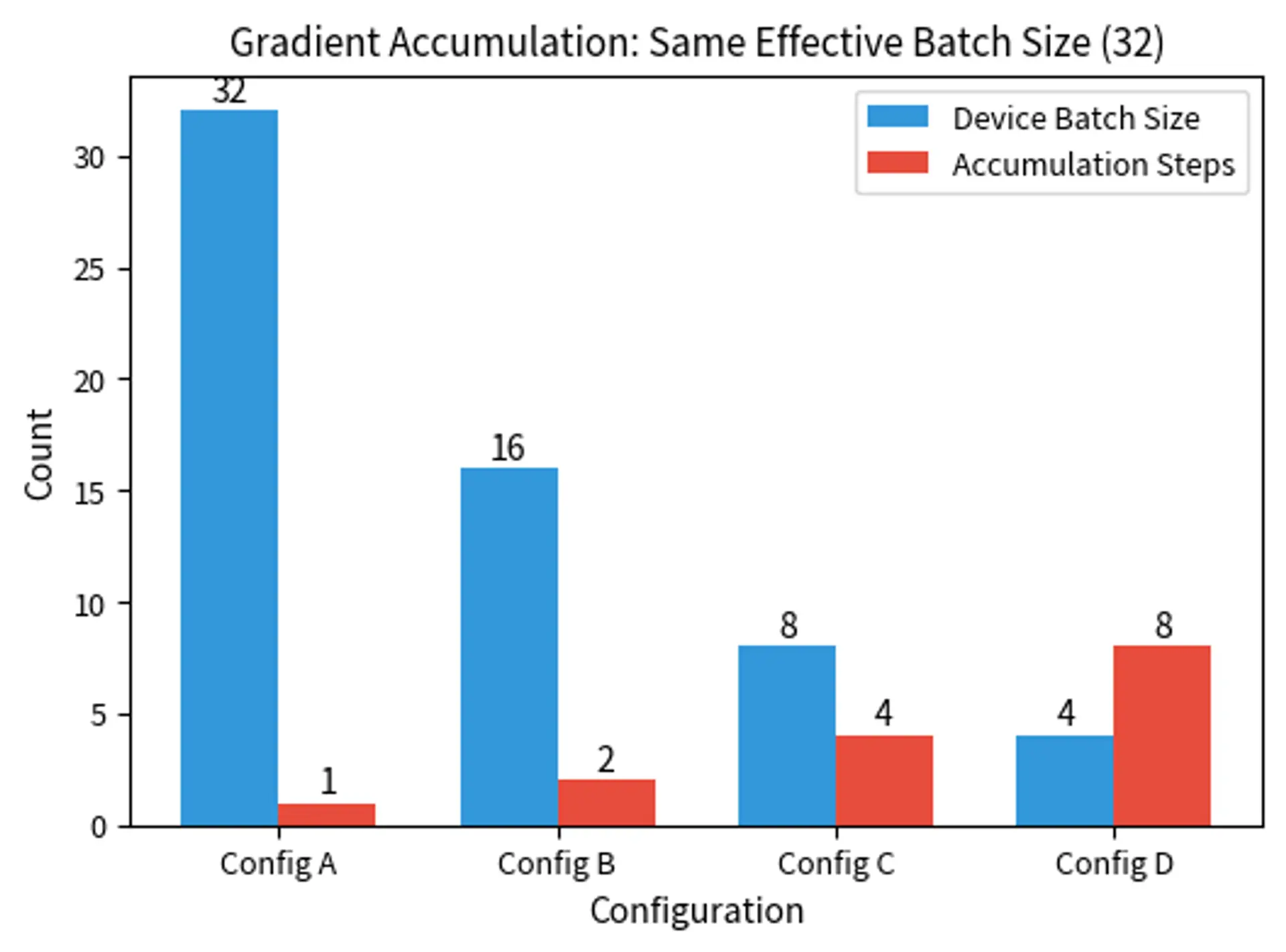
When memory constraints prevent using the desired batch size, gradient accumulation provides a workaround. Instead of updating weights after each batch, we accumulate gradients over multiple batches, then update. This technique effectively decouples the memory requirements (determined by the batch that fits in GPU memory) from the effective batch size (determined by how many batches we accumulate before updating).

If you want an effective batch size of 32 but can only fit 8 samples in memory, you accumulate gradients over 4 batches. Gradient accumulation allows us to simulate larger batch sizes by computing multiple forward and backward passes before performing a single parameter update. The relationship is expressed by the following formula:

where:

• $B_{\text{effective}}$: the effective batch size used for parameter updates (32 in this example)
• $B_{\text{device}}$: the batch size that fits in device memory (8 in this example)
• $N_{\text{accum}}$: the number of gradient accumulation steps (4 in this example)
• The multiplication: combines multiple small batches into one large gradient update, trading time for memory

This formula shows that the effective batch size equals the device batch size multiplied by the number of accumulation steps. The key insight is that gradient accumulation computes $N_{\text{accum}}$ forward and backward passes, summing the gradients before performing a single parameter update. This produces mathematically equivalent results to processing all $B_{\text{effective}}$ samples simultaneously, but uses only $B_{\text{device}}$ worth of memory at any given time. The trade-off is computational: we perform more forward and backward passes, but each pass uses less memory.

Applying this formula to our example demonstrates how the pieces fit together:

Gradient accumulation produces mathematically equivalent results to larger batches (assuming synchronized batch normalization isn't involved). The only difference is computational: accumulation requires more forward/backward passes but uses less memory per pass. This equivalence makes gradient accumulation an invaluable tool for training large models on limited hardware.

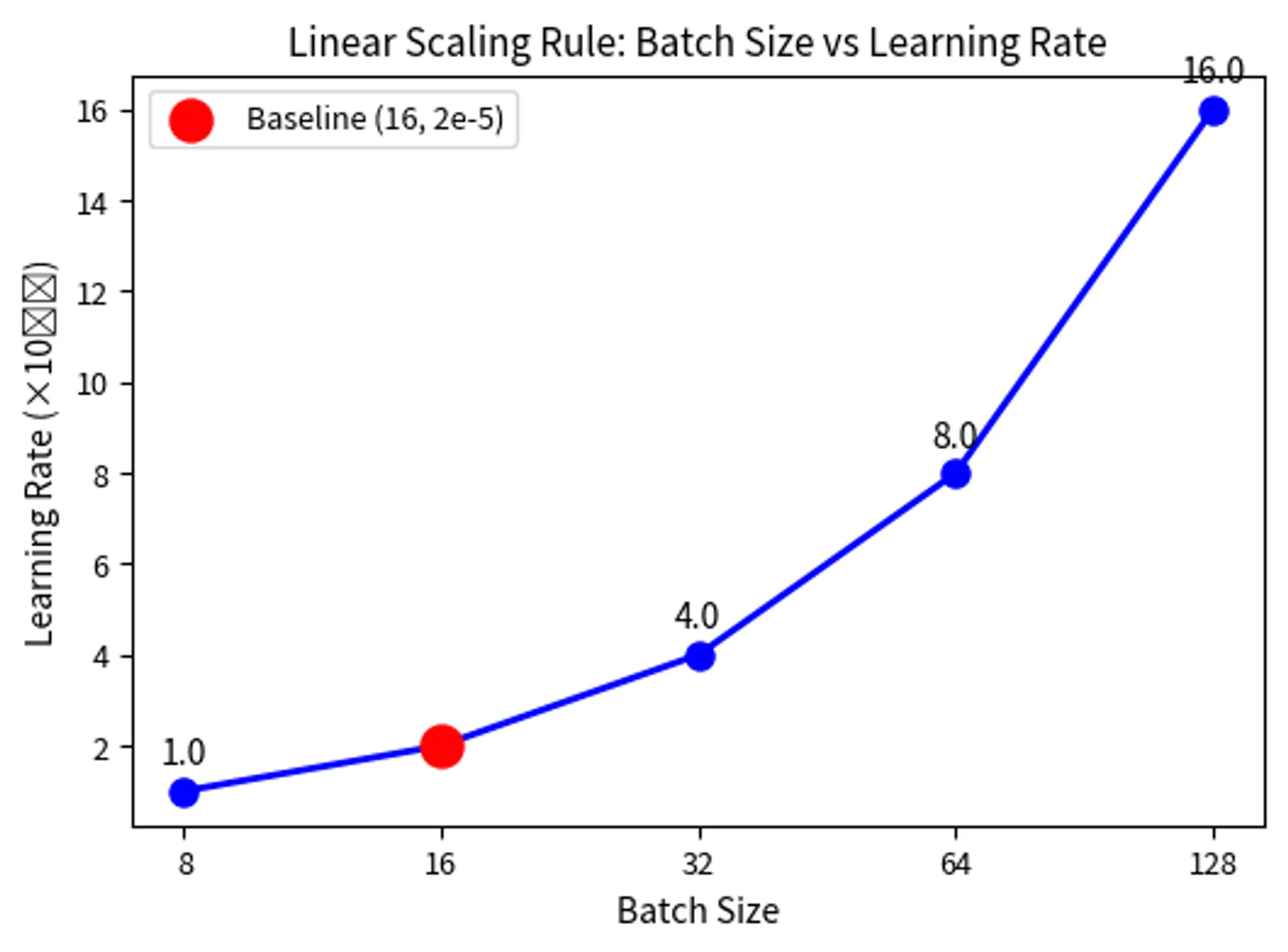
Larger batches benefit from higher learning rates. The intuition is straightforward: with more samples, the gradient estimate is more reliable, so we can take larger steps confidently. When we compute a gradient from 32 samples instead of 16, the estimate is closer to the true gradient over the full dataset, and we can trust it more. The linear scaling rule suggests that learning rate should scale proportionally with batch size according to the following relationship:

where:

• $\text{lr}_{\text{new}}$: the adjusted learning rate for the new batch size
• $\text{lr}_{\text{base}}$: the baseline learning rate that was validated with the baseline batch size
• $B_{\text{new}}$: the new batch size you want to use
• $B_{\text{base}}$: the baseline batch size used during validation
• The ratio $\frac{B_{\text{new}}}{B_{\text{base}}}$: the scaling factor by which the batch size changes

This formula adjusts the learning rate proportionally to changes in batch size. The linear scaling rule works because doubling the batch size doubles the number of samples contributing to each gradient, making the gradient estimate twice as stable. This stability allows us to take steps that are twice as large (double the learning rate) while maintaining similar training dynamics. The rule preserves the expected magnitude of parameter updates per training sample, keeping the optimization trajectory similar despite different batch sizes.

However, this rule has limits. Very large batches (thousands of samples) often fail to benefit from proportionally scaled learning rates. The relationship becomes sublinear, and other techniques like LAMB (Layer-wise Adaptive Moments) become necessary for successful training. The breakdown occurs because extremely large batches can converge to sharp minima that generalize poorly.

For fine-tuning with typical batch sizes (16-64), the linear scaling rule provides reasonable guidance. If you've validated that a learning rate of 2e-5 works well with batch size 16, then batch size 32 might benefit from 4e-5. Let's verify this by applying the linear scaling rule:

This calculation shows that doubling the batch size from 16 to 32 suggests doubling the learning rate from 2e-5 to 4e-5. The linear scaling rule provides a principled starting point, though practitioners should still validate that the scaled learning rate works well for their specific task.

Let's walk through a complete fine-tuning implementation, examining each component in detail.

While high-level APIs handle many details, understanding the underlying training loop provides insight into what's happening during fine-tuning.

Notice the parameter grouping: we apply weight decay to most parameters but exclude biases and layer normalization weights. This follows the original BERT fine-tuning recipe and prevents these parameters from being pushed toward zero unnecessarily.

Each training step involves a forward pass, loss computation, backward pass, and parameter update.

Gradient clipping prevents any single batch from causing excessively large updates. The maximum gradient norm of 1.0 is a common choice for fine-tuning, constraining the total magnitude of gradients across all parameters to prevent training instability.

Evaluating during fine-tuning helps monitor for overfitting and select the best checkpoint.

Putting it all together into a complete training run:

The training configuration shows the total number of parameter updates that will occur during fine-tuning. The warmup steps represent the initial phase where the learning rate gradually increases, helping stabilize training from the randomly initialized classification head.

The key parameters for full fine-tuning are:

• learning_rate: Controls how much weights change per update. Typically 1e-5 to 5e-5 for transformer fine-tuning.
• num_train_epochs: Number of passes through the training data. Usually 2-5 epochs for fine-tuning.
• per_device_train_batch_size: Samples per batch on each device. Common values are 16-32 for BERT-sized models.
• warmup_ratio: Fraction of training for learning rate warmup. Typically 0.06-0.1 (6-10%).
• weight_decay: L2 regularization strength. Common value is 0.01.
• gradient_accumulation_steps: Number of batches to accumulate before updating. Use to simulate larger batch sizes.

The training progresses through multiple epochs, with both training and validation metrics tracked at each step. The best model checkpoint is saved based on validation accuracy, which helps prevent overfitting by selecting the model state that generalizes best to unseen data. The final validation accuracy demonstrates how well the fine-tuned model performs on held-out examples.

Tracking loss and accuracy across epochs helps diagnose training issues.

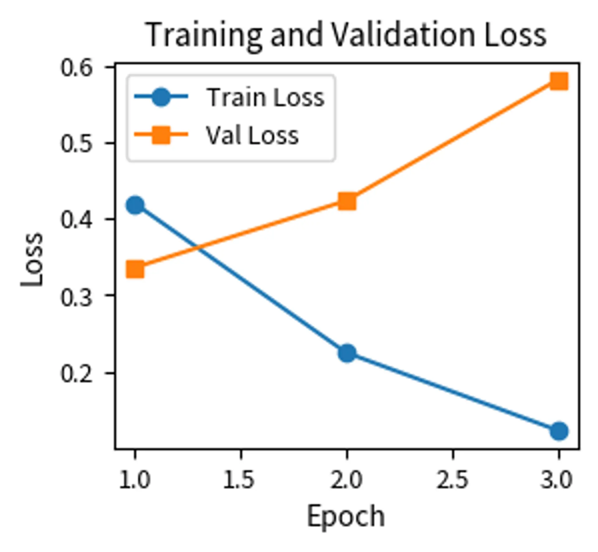
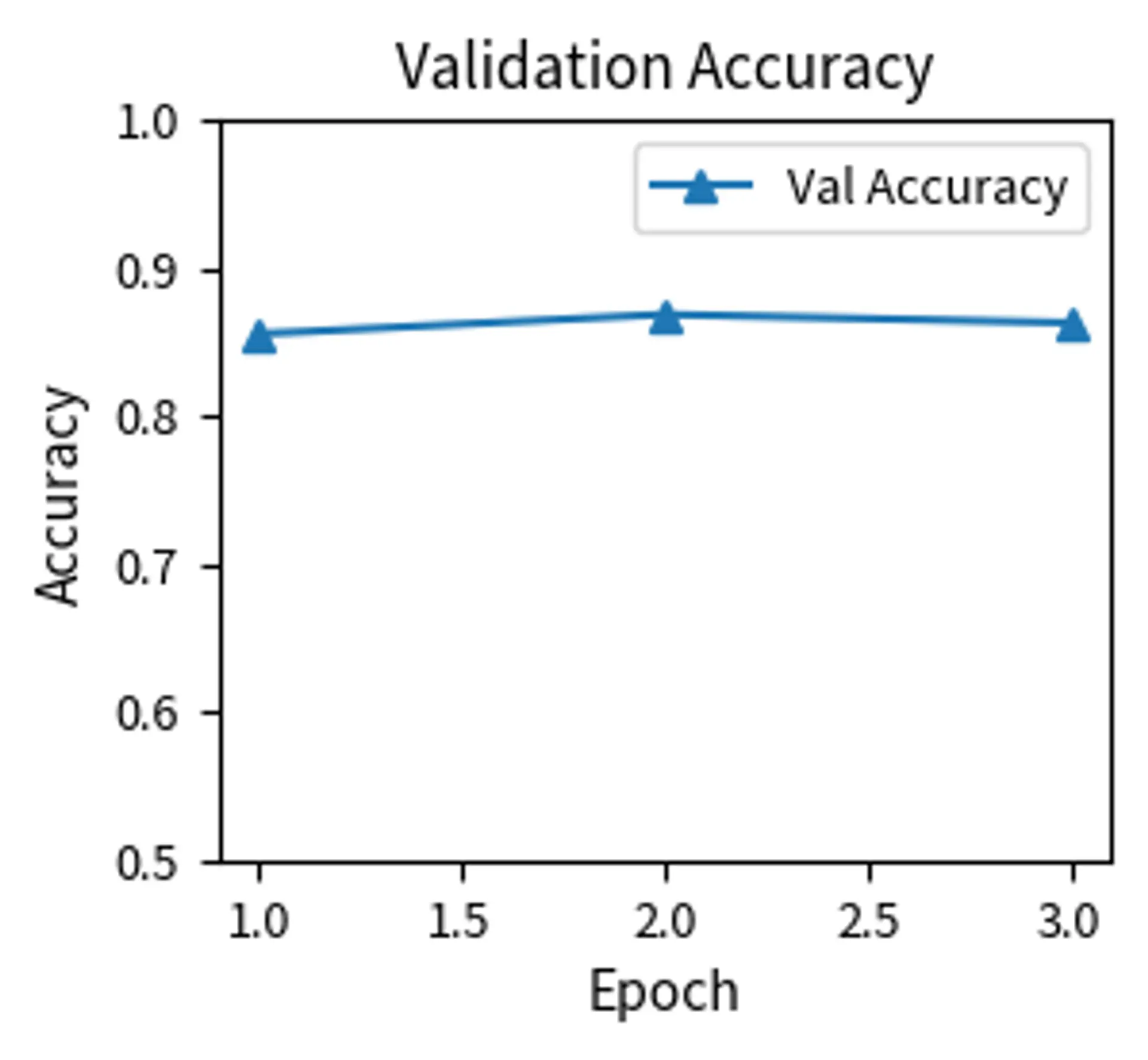
The training curves reveal the dynamics of fine-tuning. Training loss should decrease steadily. Validation loss may decrease initially but can increase if the model begins overfitting. The gap between training and validation loss indicates the degree of overfitting. These curves provide essential feedback for diagnosing issues. If validation loss increases while training loss decreases, the model is overfitting and may benefit from stronger regularization or fewer epochs.

To illustrate the impact of hyperparameter choices, let's compare different configurations.

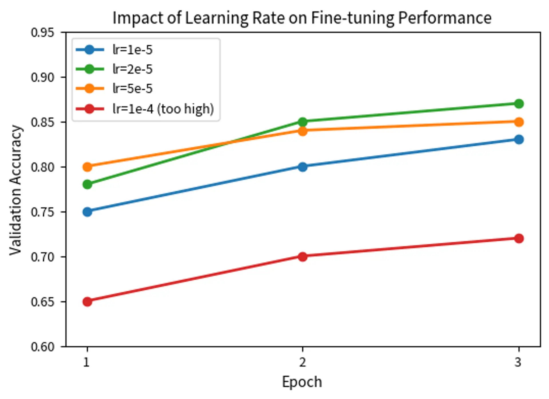
The comparison reveals several patterns characteristic of fine-tuning:

• Learning rates in the 2e-5 range typically perform best for BERT-style models
• Lower rates (1e-5) learn more slowly but can achieve good results with more epochs
• Higher rates (5e-5) may be appropriate for larger datasets where faster adaptation is beneficial
• Excessively high rates (1e-4) damage pre-trained representations and lead to poor performance

Full fine-tuning is powerful but comes with significant limitations that practitioners must understand.

Computational cost scales with model size. Fine-tuning BERT-base requires moderate resources. However, fine-tuning a 7B parameter model demands multiple high-end GPUs. Each forward and backward pass touches every parameter. Optimizer states (momentum and variance buffers) add 2-3x memory overhead for Adam-family optimizers.

where:

• Momentum buffers: exponential moving averages of past gradients, used to smooth and accelerate optimization
• Variance buffers: exponential moving averages of squared gradients, used to adapt learning rates per parameter
• 2-3x memory overhead: for each parameter of size $p$, Adam stores the parameter itself ($p$ bytes), momentum ($p$ bytes), and variance ($p$ bytes), totaling $3p$ bytes

This cost makes full fine-tuning of very large models impractical for many organizations, motivating the parameter-efficient approaches we will explore in Part XXV.

Storage requirements compound when serving multiple tasks. Each fine-tuned model is a complete copy of the original. If you fine-tune BERT for 10 different tasks, you need to store 10 complete models, each at full size. For a 3B parameter model at 16-bit precision, each task requires roughly 6GB of storage (calculated as 3 billion parameters times 2 bytes per parameter, equaling 6GB). This creates significant infrastructure challenges for multi-task deployments.

Catastrophic forgetting remains a fundamental challenge. As the model adapts to new data, it can lose capabilities from pre-training. A model fine-tuned heavily on medical text might perform worse on general language understanding than the original. We will examine this phenomenon in detail in the next chapter, covering why it occurs and techniques to mitigate it.

Despite these limitations, full fine-tuning remains the gold standard for maximum task performance. When you have sufficient compute, storage, and task-specific data, full fine-tuning typically outperforms parameter-efficient alternatives. The entire model can adapt its representations to the target domain, creating highly specialized capabilities.

Full fine-tuning adapts all parameters of a pre-trained model to a downstream task. The procedure involves loading a pre-trained checkpoint, adding a task-specific head, and training on labeled data with carefully selected hyperparameters.

Here are the critical hyperparameters for fine-tuning:

• Learning rate: typically $1 \times 10^{-5}$ to $5 \times 10^{-5}$ (much lower than pre-training rates)
• Number of epochs: usually 2-5 (just enough for adaptation without overfitting)
• Batch size: 16-32 for consumer GPUs. Use gradient accumulation for larger effective sizes.
• Warmup ratio: 0.06 to 0.1 (6% to 10%) of training steps to stabilize early training
• Weight decay: Around 0.01, applied to most but not all parameters

Learning rate schedules like linear or cosine decay, combined with warmup, provide stable training dynamics. The batch size-learning rate relationship suggests scaling both together for consistent behavior.

Full fine-tuning excels when compute resources are available and maximum task performance is the goal. For resource-constrained scenarios or multi-task deployments, parameter-efficient methods offer attractive alternatives. In the following chapters, we'll examine catastrophic forgetting in depth and explore learning rate strategies that can further improve fine-tuning results.

Ready to test your understanding? Take this quick quiz to reinforce what you've learned about full fine-tuning.