Layer Normalization: Stabilizing Transformer Training

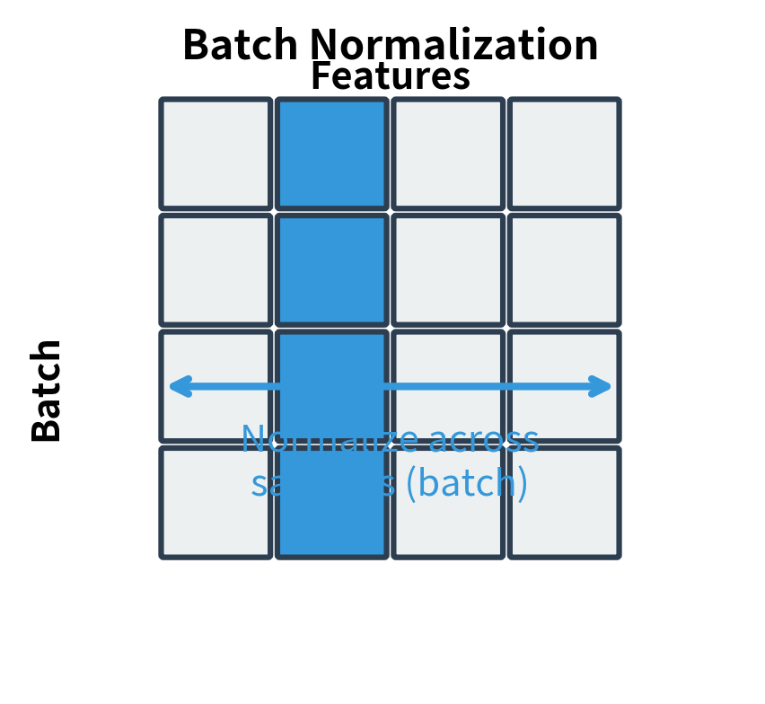
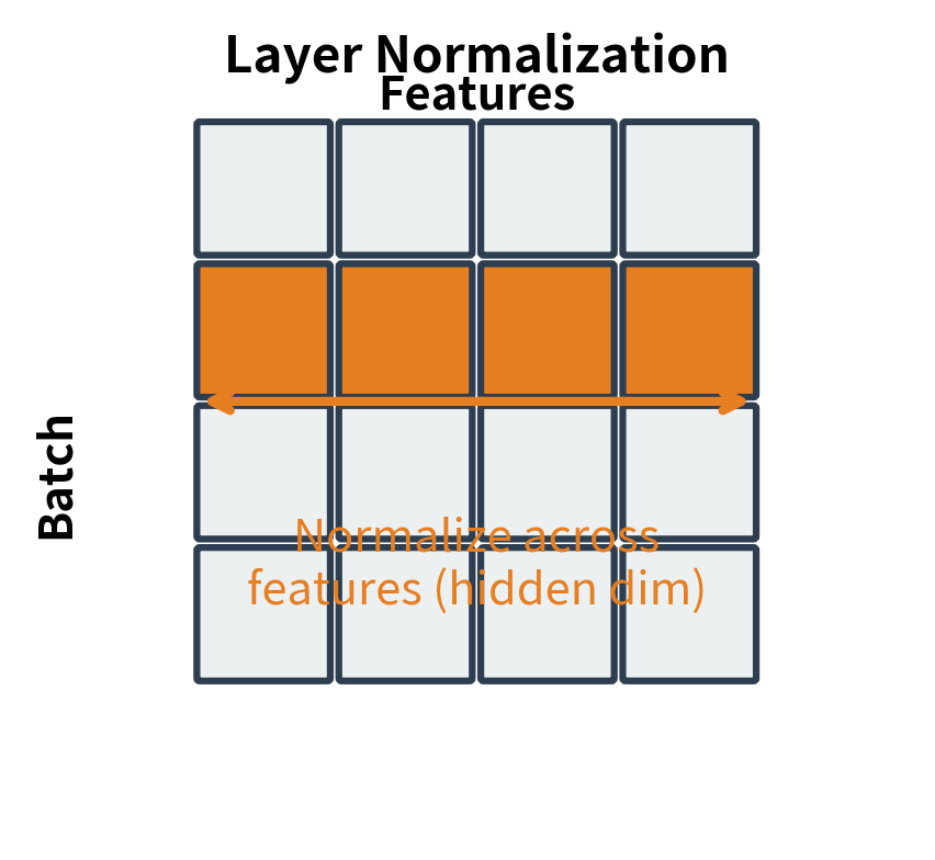
Batch normalization transformed how we train deep feedforward networks, but it stumbles when applied to transformers. The batch dimension becomes problematic: batch sizes vary, sequences have different lengths, and the statistics computed across a batch of diverse sentences lack semantic coherence. Layer normalization, introduced by Ba, Kiros, and Hinton in 2016, sidesteps these issues entirely by normalizing across features rather than across the batch. This seemingly simple change made layer normalization the default normalization technique for transformers, from the original "Attention is All You Need" architecture to modern large language models.

In this chapter, we'll explore why layer normalization works so well for transformers, how it differs from batch normalization in both computation and behavior, and the subtle implementation details that affect training stability. We'll also examine how the placement of layer normalization within transformer blocks affects learning dynamics, a design choice that has evolved significantly since the original transformer architecture.

Before diving into layer normalization, it's worth understanding exactly why batch normalization doesn't work well for sequence models. The core issue is that batch normalization computes statistics across the batch dimension, assuming that each position in a layer sees similar data across samples.

In a transformer processing sentences of varying lengths, each position in the sequence represents something different. Position 0 might be "The" in one sentence and "Scientists" in another. Position 50 might be a verb in one sentence, a noun in another, and padding in a third. Computing a mean and variance across these semantically unrelated positions produces statistics that don't reflect any meaningful property of the data.

The batch statistics are dominated by the extreme sequences, and these statistics change dramatically between positions. Layer normalization avoids this problem entirely by computing statistics within each sample independently, treating each token's representation as a self-contained unit to normalize.

To understand layer normalization, let's start with a fundamental question: what does it mean for a neural network layer to have "unstable" activations, and how can we fix it?

Imagine a token's hidden representation as a vector of 768 numbers (a typical transformer dimension). During training, these numbers can drift: some become very large, others very small, and their collective distribution shifts unpredictably. This creates two problems. First, downstream layers must constantly adapt to changing input statistics, making learning inefficient. Second, when values grow too large or too small, gradients either explode or vanish, destabilizing training entirely.

The solution is elegant: before each token's representation moves to the next layer, we transform it to have a predictable, standardized distribution. Specifically, we want the 768 features to have zero mean and unit variance. This "resets" the scale at every layer, preventing drift from accumulating.

The first step is computing where the current distribution is centered. Given a hidden state vector $\mathbf{x} = [x_1, x_2, \ldots, x_d]$ representing one token, we calculate its mean:

where:

• $\mu$: the arithmetic mean of all $d$ features in this token's representation
• $d$: the hidden dimension (e.g., 768 for BERT-base, 4096 for LLaMA-7B)
• $x_i$: the value of the $i$-th feature

This tells us the "center of mass" of the representation. If $\mu = 2.5$, the features are shifted toward positive values; if $\mu = -1.3$, they lean negative. The goal is to shift this center to zero.

Next, we need to know how spread out the values are. A representation where all values cluster tightly around the mean is very different from one where values are scattered widely. We capture this with variance:

where:

• $\sigma^2$: the variance, measuring how much the features deviate from their mean
• $(x_i - \mu)^2$: the squared deviation of each feature from the mean

Squaring ensures that positive and negative deviations don't cancel out. If $\sigma^2$ is large, the features are spread out; if small, they're tightly clustered. We'll use the standard deviation $\sigma = \sqrt{\sigma^2}$ to rescale the values to unit variance.

With mean and variance in hand, we can now standardize each feature:

where:

• $\hat{x}_i$: the normalized value of the $i$-th feature
• $\epsilon$: a tiny constant (typically $10^{-5}$) added to prevent division by zero if variance is extremely small

This two-part transformation is exactly what you'd do to standardize any dataset: subtract the mean (centering at zero), then divide by the standard deviation (scaling to unit variance). The result $\hat{x}_i$ has zero mean and approximately unit variance across the $d$ features.

Here's where layer normalization becomes clever rather than restrictive. Forcing every representation to have exactly zero mean and unit variance might seem limiting: what if the optimal representation for some layer actually needs a different distribution?

The solution is to add learnable parameters that can undo the normalization if needed:

where:

• $y_i$: the final output for the $i$-th feature
• $\gamma_i$: a learned scale parameter for feature $i$ (initialized to 1)
• $\beta_i$: a learned shift parameter for feature $i$ (initialized to 0)

These parameters are learned during training, just like weights and biases. If the network discovers that feature $i$ should have mean 3.5 and standard deviation 2.0, it can learn $\gamma_i = 2.0$ and $\beta_i = 3.5$ to recover that distribution. This means layer normalization never reduces the network's representational power: it starts from a stable baseline but can learn any distribution it needs.

Putting all the pieces together, layer normalization transforms a hidden state vector $\mathbf{x}$ of dimension $d$ into:

where:

• $\mathbf{x} = [x_1, x_2, \ldots, x_d]$: the input vector representing one token's hidden state
• $\mu = \frac{1}{d} \sum_{i=1}^{d} x_i$: the mean across all features
• $\sigma^2 = \frac{1}{d} \sum_{i=1}^{d} (x_i - \mu)^2$: the variance across all features
• $\epsilon$: a small stability constant (typically $10^{-5}$ or $10^{-6}$)
• $\gamma = [\gamma_1, \gamma_2, \ldots, \gamma_d]$: learned scale parameters, initialized to ones
• $\beta = [\beta_1, \beta_2, \ldots, \beta_d]$: learned shift parameters, initialized to zeros
• $\odot$: element-wise multiplication

The formula reads naturally: subtract the mean, divide by the standard deviation (with a safety epsilon), then apply a learned scale and shift.

The key insight that distinguishes layer normalization from batch normalization is the dimension over which we compute statistics. Batch normalization asks: "What's the typical value of feature $i$ across all samples in this batch?" Layer normalization asks: "What's the typical value across all features for this particular token?"

For transformers, the layer normalization approach is far more natural. Each token is processed independently, and we want stable statistics regardless of what other tokens or samples happen to be in the batch. This independence also means layer normalization works identically during training and inference, with no need for running statistics or batch size considerations.

Now that we understand the formula conceptually, let's translate it into code. Building layer normalization from scratch will solidify our understanding and reveal the implementation details that matter in practice.

Our implementation follows the mathematical steps exactly: compute mean, compute variance, normalize, then apply the learnable transformation.

The dim=-1 argument tells PyTorch to compute statistics across the last dimension (features), which is exactly what layer normalization requires. The keepdim=True preserves the dimension for broadcasting during subtraction and division.

Let's trace through layer normalization with concrete numbers to see exactly what happens at each step.

The input tokens have varying means (around 2-3) and standard deviations (around 2-4), reflecting the non-standard distribution we created. After layer normalization, each token has mean essentially zero and standard deviation essentially one. The tiny deviations from exactly 0 and 1 are floating-point precision artifacts, not algorithmic issues.

Let's visualize this transformation to see exactly how layer normalization reshapes the feature distribution.

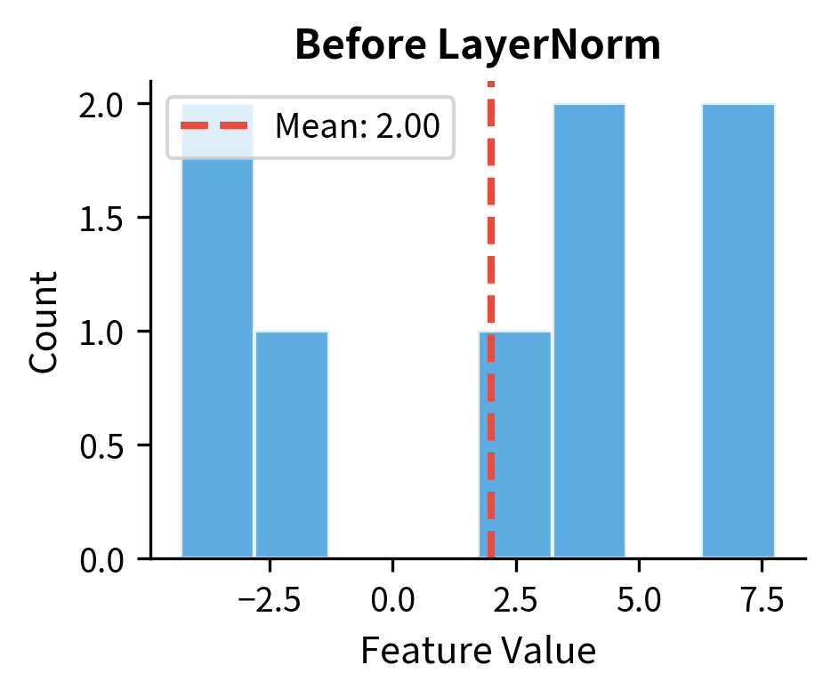
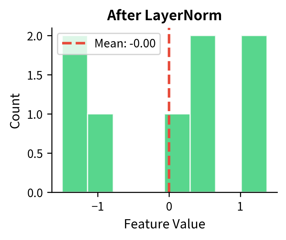
The histograms make the transformation crystal clear. Before normalization, the feature values are scattered around a positive mean with varied spread. After normalization, they're centered at zero with approximately unit variance. This happens independently for every token in the sequence.

Notice that each token is normalized independently: the first token's statistics don't affect the second token's normalization. This independence is precisely what makes layer normalization suitable for transformers, where tokens must be processed in parallel and sequences have variable lengths.

After normalizing activations to zero mean and unit variance, we've effectively forced all features into a standardized distribution. But what if the network actually needs some features to have a larger spread, or to be centered around a non-zero value? The learnable parameters $\gamma$ (scale) and $\beta$ (shift) solve this problem.

For each feature dimension $i$, the final output is:

where:

• $y_i$: the final output for the $i$-th feature
• $\hat{x}_i$: the normalized value (zero mean, unit variance)
• $\gamma_i$: the learned scale for feature $i$, which controls the spread of values
• $\beta_i$: the learned shift for feature $i$, which controls the center of the distribution

Here's the key insight: if the network learns $\gamma_i = \sigma_{\text{original}}$ and $\beta_i = \mu_{\text{original}}$, it can completely undo the normalization and recover the original distribution. This means layer normalization can never hurt the network's representational capacity; in the worst case, it learns to bypass itself entirely. In practice, the network finds an intermediate setting that benefits from stable optimization while still representing the patterns it needs.

The output distribution for each feature is controlled by its corresponding $\gamma$ and $\beta$ values. Features with larger $\gamma$ values have wider distributions, while $\beta$ shifts the center. This per-feature control allows different dimensions of the representation to operate at different scales, which is crucial for transformers where different attention heads and feature dimensions may need different dynamic ranges.

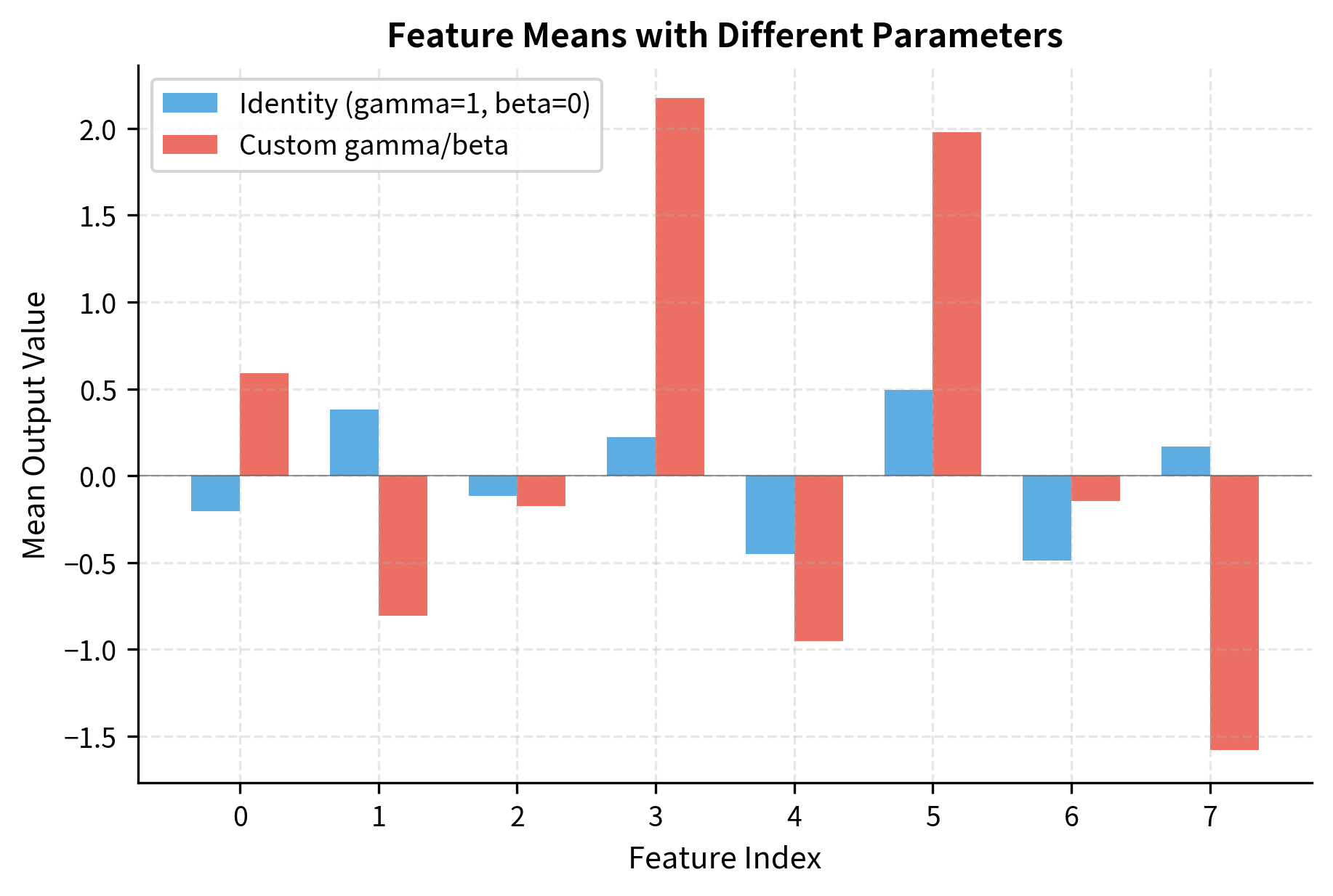
With identity parameters (gamma=1, beta=0), all feature means are near zero as expected. With custom parameters, each feature shifts to its corresponding beta value, demonstrating how the learnable parameters give each dimension independent control over its output distribution.

PyTorch provides a built-in nn.LayerNorm that handles all these details efficiently. Let's verify our implementation matches PyTorch's behavior.

The outputs match within floating-point precision, confirming our implementation is correct.

In transformer architectures, layer normalization appears in two key locations: after the attention mechanism and after the feed-forward network. The original transformer used "post-norm" placement, where normalization comes after the residual connection:

Modern architectures like GPT-2, GPT-3, and LLaMA use "pre-norm" placement, where normalization comes before the sublayer:

The difference in placement has significant implications for gradient flow, which we'll explore in detail in the pre-norm vs post-norm chapter.

Understanding how gradients flow through layer normalization is essential for debugging training issues and understanding why normalization stabilizes training.

The backward pass through layer normalization is more complex than a simple element-wise operation because each output depends on all inputs through the mean and variance computation. When we change a single input $x_i$, it affects not only its own normalized output but also the mean $\mu$ and variance $\sigma^2$, which in turn affect every output element. This coupling makes the gradient computation more intricate.

Given the loss $L$ and the upstream gradient $\frac{\partial L}{\partial y}$ (the gradient flowing back from later layers), we need to compute three gradients: $\frac{\partial L}{\partial x}$ for backpropagation, and $\frac{\partial L}{\partial \gamma}$ and $\frac{\partial L}{\partial \beta}$ for updating the learnable parameters.

The output of layer normalization is $y_i = \gamma_i \cdot \hat{x}_i + \beta_i$, where $\hat{x}_i$ is the normalized input. Since this is a simple affine transformation, the gradients follow directly from the chain rule.

For the scale parameter $\gamma_i$:

where:

• $\frac{\partial L}{\partial \gamma_i}$: the gradient of the loss with respect to the $i$-th scale parameter
• $n$: an index over all tokens (across batch and sequence dimensions)
• $\frac{\partial L}{\partial y_{n,i}}$: the upstream gradient for the $i$-th feature of the $n$-th token
• $\hat{x}_{n,i}$: the normalized value of the $i$-th feature for the $n$-th token

Intuitively, this sums up how much each token's normalized value contributed to the loss through this scale parameter.

For the shift parameter $\beta_i$:

where:

• $\frac{\partial L}{\partial \beta_i}$: the gradient of the loss with respect to the $i$-th shift parameter

This is simply the sum of upstream gradients, since $\beta_i$ adds directly to the output.

The gradient with respect to input is more involved because $\hat{x}_i$ depends on $x_i$ in three ways: directly, through the mean $\mu$, and through the variance $\sigma^2$. Applying the chain rule carefully yields:

where:

• $\frac{\partial L}{\partial x_i}$: the gradient of the loss with respect to the $i$-th input element
• $\gamma_i$: the learned scale parameter for the $i$-th feature
• $\sigma = \sqrt{\sigma^2 + \epsilon}$: the standard deviation (with epsilon for stability)
• $d$: the feature dimension (number of elements in the input vector)
• $\hat{x}_i$: the normalized input, equal to $(x_i - \mu) / \sigma$

Let's break down the three terms inside the parentheses:

1. Direct contribution $\frac{\partial L}{\partial y_i}$: The gradient that would flow if normalization were a simple scaling operation.

2. Mean correction $-\frac{1}{d}\sum_{j=1}^{d}\frac{\partial L}{\partial y_j}$: Accounts for how changing $x_i$ affects $\mu$, which affects all outputs. This term subtracts the average gradient, centering the gradient distribution.

3. Variance correction $-\frac{\hat{x}_i}{d}\sum_{j=1}^{d}\frac{\partial L}{\partial y_j}\hat{x}_j$: Accounts for how changing $x_i$ affects $\sigma^2$, which scales all outputs. This term is proportional to the normalized value $\hat{x}_i$, meaning inputs far from the mean get larger corrections.

This formula reveals something important: the gradient for each input element depends on the gradients of all other elements through the mean and variance terms. This coupling helps distribute gradient information across features, which can improve training stability.

The differences are on the order of $10^{-7}$ or smaller, well within floating-point precision. This confirms our manual backward pass implementation correctly computes the gradients that PyTorch's autograd produces automatically.

Let's visualize how layer normalization transforms the activation distribution during a forward pass through multiple transformer blocks.

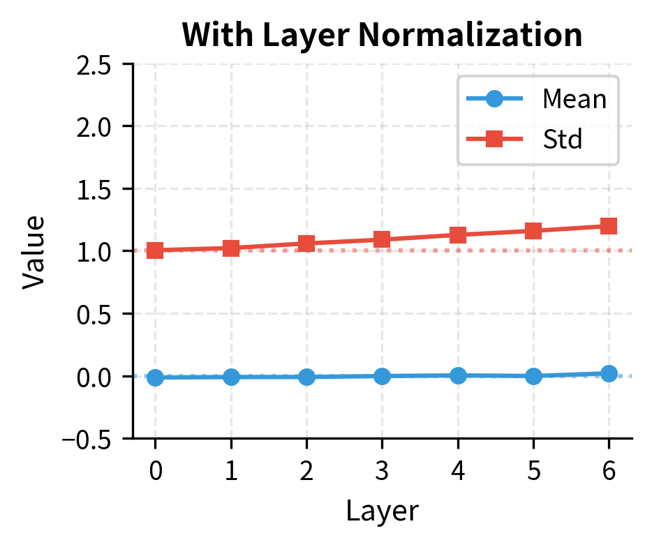
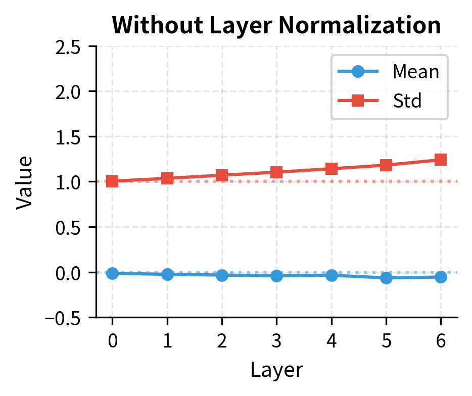
With layer normalization, activations maintain stable statistics throughout the network. Without it, activations can drift, though the effect depends heavily on initialization. In practice, this stability becomes crucial during training when weight updates can cause activation statistics to shift dramatically without normalization to anchor them.

The epsilon parameter ($\epsilon$) appears in the denominator of the normalization formula:

where:

• $\hat{x}_i$: the normalized value for the $i$-th feature
• $x_i$: the original input value
• $\mu$: the mean across all features
• $\sigma^2$: the variance across all features
• $\epsilon$: a small constant added to prevent division by zero

The purpose of $\epsilon$ is to ensure numerical stability. If all input values are identical (or nearly so), the variance $\sigma^2$ approaches zero. Without $\epsilon$, we would divide by zero, producing infinity or NaN. Adding a small positive constant like $10^{-5}$ ensures the denominator is always positive.

The choice of epsilon can affect numerical stability, especially with mixed-precision (FP16) training where very small values may underflow.

The input variance is extremely small (around $10^{-8}$), which means we're dividing by a very small number. With epsilon = 0, the output standard deviation explodes because we're essentially dividing by nearly zero. As epsilon increases, the output becomes more stable. The standard choice of $10^{-5}$ strikes a balance: it's large enough to prevent numerical issues but small enough not to distort the normalization when variance is reasonably sized. A reasonable epsilon value (typically $10^{-5}$ to $10^{-6}$) provides a safety net without affecting normal computations.

PyTorch's nn.LayerNorm accepts a normalized_shape parameter that controls which dimensions are normalized. For transformers, we typically normalize over the feature dimension only:

Notice the difference: with normalized_shape=(8,), each individual token has zero mean (Token 0,0 and Token 0,1 both have mean approximately 0). With normalized_shape=(4, 8), the entire sample is normalized together, so individual tokens may have non-zero means but the sample as a whole has zero mean.

Normalizing over features only is the standard choice for transformers because it treats each token independently, matching the autoregressive nature of language models and allowing the model to process variable-length sequences.

Layer normalization has become ubiquitous in transformer architectures, but it's not without drawbacks.

The primary computational overhead comes from computing statistics for every token at every layer. For a model with hidden dimension $d$, each layer normalization requires computing a mean (sum of $d$ elements) and variance (sum of $d$ squared differences), then normalizing all $d$ elements. While these operations are memory-bandwidth bound rather than compute-bound on modern GPUs, they still add up in models with hundreds of layers.

The learned $\gamma$ and $\beta$ parameters add $2d$ parameters per layer normalization, which is negligible compared to attention and FFN parameters but contributes to model complexity. More importantly, these parameters can be a source of numerical issues when they grow very large or approach zero, requiring careful initialization and sometimes explicit constraints.

Layer normalization also introduces a subtle form of coupling between features that can affect interpretability. Because each feature is normalized relative to the others, the absolute activation value of any single feature becomes less meaningful. This makes it harder to interpret individual neurons or feature dimensions in isolation.

Despite these limitations, layer normalization's impact on transformer training stability cannot be overstated. Before normalization techniques were widely adopted, training deep networks required careful learning rate tuning, extensive warmup periods, and often failed entirely for very deep models. Layer normalization enables stable training with higher learning rates, reduces sensitivity to initialization, and allows models to scale to unprecedented depths. The original transformer used layer normalization, and every major language model since has relied on some form of normalization to train successfully.

The success of layer normalization has also spurred research into alternatives. RMSNorm, which we'll cover in the next chapter, removes the mean-centering step to improve computational efficiency while maintaining most of the stability benefits.

When using nn.LayerNorm in PyTorch, understanding the key parameters helps you configure it correctly for your architecture:

• normalized_shape: The shape of the input over which to normalize. For transformers, this is typically the hidden dimension d_model (e.g., 768, 1024). You can also pass a list like [seq_len, d_model] to normalize over multiple dimensions, though normalizing over features only is the standard choice.

• eps: The epsilon value added to the denominator for numerical stability. Default is 1e-5, which works well for most cases. For mixed-precision (FP16) training, you may need a larger value like 1e-4 to avoid underflow issues when variance is very small.

• elementwise_affine: Whether to include learnable $\gamma$ and $\beta$ parameters. Default is True. Setting to False removes the learnable parameters, reducing model size slightly but limiting the network's ability to learn optimal feature scales.

Layer normalization is a fundamental component of transformer architectures that enables stable training of deep models. Unlike batch normalization, which computes statistics across the batch dimension, layer normalization operates on each sample independently, making it well-suited for variable-length sequences and small batch sizes.

The core operation normalizes each token's representation to zero mean and unit variance, then applies learned scale ($\gamma$) and shift ($\beta$) parameters to recover representational flexibility. This simple transformation stabilizes activations throughout the network, prevents gradient issues during training, and reduces sensitivity to initialization.

Key takeaways:

• Feature-wise normalization: Layer normalization computes mean and variance across the feature dimension, treating each token independently
• Learnable parameters: $\gamma$ and $\beta$ allow the network to undo normalization when beneficial, preserving representational capacity
• Placement matters: Pre-norm (normalize before sublayer) has become the modern standard, improving gradient flow in deep networks
• Epsilon for stability: A small constant prevents division by zero with near-constant inputs
• No batch dependency: Works with any batch size, including single samples during inference

Ready to test your understanding? Take this quick quiz to reinforce what you've learned about layer normalization in transformers.