Relative Position Encoding: Distance-Based Attention for Transformers

Previous chapters explored absolute position encoding: each position receives a fixed representation based on its index in the sequence. Whether through sinusoidal functions or learned embeddings, the model learns that "position 5 means something specific." But language doesn't work this way. When you read "the cat sat on the mat," the relationship between "cat" and "sat" depends on their relative distance (one word apart), not on whether they appear at positions 2 and 3 versus positions 102 and 103.

Relative position encoding shifts the focus from "where am I?" to "how far apart are we?" This chapter explores why this matters, how to formulate relative attention, and how Shaw et al.'s influential approach brought relative positions into transformer self-attention.

Consider the sentence "The cat that I saw yesterday sat on the mat." The verb "sat" needs to find its subject "cat." With absolute position encoding, the model must learn that "position 5 attending to position 2" captures a subject-verb relationship. But if we move the same phrase later in the document, it becomes "position 105 attending to position 102." The model must learn these patterns for every possible absolute position pair.

Relative position encoding solves this by focusing on the offset between positions. The distance from position 5 to position 2 is $-3$ (looking backward three positions). The distance from position 105 to position 102 is also $-3$. By encoding this offset rather than absolute positions, the model learns a single pattern for "three positions back" that generalizes across the entire sequence.

This shift has practical consequences. Language has many distance-dependent patterns: adjectives typically appear one position before their nouns, determiners precede noun phrases by a few positions, and verbs often follow their subjects within a local window. Relative encoding captures these patterns directly.

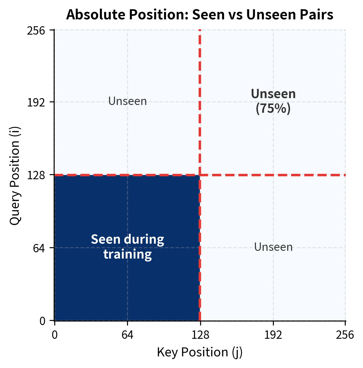
Nearly 75% of position pairs at test time were never seen during training. A model relying on absolute positions must somehow generalize to these unseen combinations. With relative encoding, every distance seen during training transfers to all positions at that distance.

Recall the standard self-attention formula. Given queries $\mathbf{Q}$, keys $\mathbf{K}$, and values $\mathbf{V}$, we compute:

where:

• $\mathbf{Q} \in \mathbb{R}^{n \times d_k}$: query matrix containing all query vectors
• $\mathbf{K} \in \mathbb{R}^{n \times d_k}$: key matrix containing all key vectors
• $\mathbf{V} \in \mathbb{R}^{n \times d_v}$: value matrix containing all value vectors
• $d_k$: dimension of queries and keys
• $\sqrt{d_k}$: scaling factor to prevent dot products from growing too large
• $n$: sequence length

With absolute position encoding, each token's embedding includes position information before the QKV projections. Position is baked into the input: $\mathbf{x}_i = \mathbf{e}_i + \mathbf{p}_i$, where $\mathbf{e}_i$ is the token embedding and $\mathbf{p}_i$ is the position encoding. The attention scores then implicitly depend on absolute positions through the projected queries and keys.

Relative position encoding takes a different approach: inject position information directly into the attention computation. Instead of adding position to the input, we modify how attention scores are calculated to explicitly account for the offset $j - i$ between positions $i$ and $j$.

The core idea is to add a position-dependent term to the attention score:

where:

• $\mathbf{q}_i$: the query vector at position $i$
• $\mathbf{k}_j$: the key vector at position $j$
• $\text{relative\_bias}(i, j)$: a term that depends only on the offset $j - i$

This formulation separates content matching ($\mathbf{q}_i \cdot \mathbf{k}_j$) from position matching (the relative bias). The model can learn that certain offsets are generally more or less important, regardless of absolute position.

The most influential formulation of relative positions in self-attention comes from Shaw et al. (2018). Their approach asks a fundamental question: if we want attention to be distance-aware, where exactly should we inject position information? Rather than modifying the input embeddings, Shaw et al. discovered that injecting relative positions directly into the attention computation gives the model finer control over how distance affects both which tokens get attention and what information flows.

To understand their approach, we need to build up three connected ideas: what we want the model to learn about distance, how to represent those distances as learnable parameters, and how to integrate those representations into the attention mechanism itself.

Consider what happens when position $i$ attends to position $j$ in standard self-attention. The model computes a score based on content similarity, then uses that score to weight how much of $j$'s information flows to $i$. But we want distance to influence both of these operations:

1. Which positions get attention: A verb might prefer to attend to positions 1-3 positions back (where subjects typically appear), regardless of content similarity.

2. What information flows: When aggregating information, we might want "nearby context" to carry different weight than "distant context," even when attention weights are equal.

Shaw et al. address both needs by introducing two sets of learnable embeddings: one that modifies attention scores, and one that modifies value aggregation. This separation gives the model independent control over "who to attend to" versus "what to gather."

For each possible offset $r = j - i$ between positions, Shaw et al. define learnable vectors:

• $\mathbf{a}^K_r \in \mathbb{R}^{d_k}$: a relative position embedding that influences attention scores
• $\mathbf{a}^V_r \in \mathbb{R}^{d_v}$: a relative position embedding that modifies aggregated values

where:

• $r = j - i$: the relative offset (positive means looking forward, negative means looking backward)
• $d_k$: dimension of query and key vectors
• $d_v$: dimension of value vectors

These embeddings are learned during training, just like the QKV projection matrices. The critical insight is that the number of distinct offsets is bounded by the sequence length (from $-(n-1)$ to $+(n-1)$), not by the number of position pairs (which is $n^2$). This means the model learns a single pattern for "three positions back" that applies universally, rather than learning separate patterns for every pair of absolute positions.

Let's trace through how relative positions enter the attention computation. In standard self-attention, the score measuring how much position $i$ should attend to position $j$ is:

where:

• $e_{ij}$: the raw attention score from query position $i$ to key position $j$
• $\mathbf{q}_i \in \mathbb{R}^{d_k}$: the query vector at position $i$
• $\mathbf{k}_j \in \mathbb{R}^{d_k}$: the key vector at position $j$
• $d_k$: the dimension of query and key vectors

This score depends only on the content at each position. Two identical words at different positions produce identical scores, regardless of their distance.

Shaw et al. modify this by adding the relative position embedding to the key before computing the dot product:

Why add to the key rather than the query? The key represents "what this position offers," so adding position information to it means the model can learn that positions at certain distances offer something different, even if their content is identical. The query remains focused on "what I'm looking for."

Expanding the dot product reveals the two-component structure:

where:

• $\mathbf{q}_i \cdot \mathbf{k}_j$: the content term, measuring semantic compatibility between positions
• $\mathbf{q}_i \cdot \mathbf{a}^K_{j-i}$: the position term, encoding how relative distance affects the score
• $\mathbf{a}^K_{j-i} \in \mathbb{R}^{d_k}$: the learned relative position embedding for offset $(j-i)$

The position term is a dot product between the query and the relative position embedding. This means different queries can respond differently to the same distance. A query learned to find subjects might have high dot product with $\mathbf{a}^K_{-2}$ (two positions back), while a query learned to find objects might prefer $\mathbf{a}^K_{+1}$ (one position forward). The model learns these patterns from data.

Shaw et al. apply the same principle to value aggregation. After computing attention weights $\alpha_{ij} = \text{softmax}(e_{ij})$, standard attention aggregates values as a weighted sum. The modified version adds relative position embeddings to the values:

where:

• $\mathbf{o}_i \in \mathbb{R}^{d_v}$: output vector at position $i$, now enriched with position-aware context
• $\alpha_{ij}$: attention weight from position $i$ to position $j$ (sums to 1 across $j$)
• $\mathbf{v}_j \in \mathbb{R}^{d_v}$: value vector at position $j$, carrying the content to aggregate
• $\mathbf{a}^V_{j-i} \in \mathbb{R}^{d_v}$: relative position embedding for values at offset $(j-i)$
• $n$: sequence length

This modification means the output at each position incorporates not just the weighted content from other positions, but also position-dependent information about where that content came from. Even if two positions have identical values and identical attention weights, their contributions differ based on their relative distances.

The two sets of embeddings ($\mathbf{a}^K$ and $\mathbf{a}^V$) work together but serve distinct roles. The key embeddings affect which positions receive attention (the "routing" decision). The value embeddings affect what information flows once routing is decided (the "content" decision). This separation allows the model to learn, for example, that adjacent positions should receive high attention (key embedding effect) while also learning that adjacent context should contribute a specific "locality" signal to the output (value embedding effect).

The formulation above assumes we have a separate embedding for every possible relative position. But this creates a practical problem: for a sequence of length $n$, relative positions range from $-(n-1)$ to $(n-1)$, requiring $2n-1$ embeddings. For a sequence of length 512, that's 1023 different embeddings per dimension, for both keys and values.

This approach has two flaws. First, memory grows linearly with sequence length. Second, distant positions appear infrequently during training. In a 128-token sequence, only one position pair has offset $+127$ (position 0 to position 127), while thousands of pairs have offset $+1$. The embedding for offset $+127$ would be severely undertrained.

Shaw et al. address both problems with a simple insight: fine-grained distance matters more locally than globally. The difference between "3 positions back" and "4 positions back" may be linguistically significant, as it could distinguish an adjective-noun relationship from a determiner-noun relationship. But the difference between "100 positions back" and "101 positions back" rarely carries meaning. Both are simply "far away."

This motivates clipping: relative positions beyond a maximum distance $k$ are clamped to $\pm k$:

where:

• $j - i$: the raw relative position (offset from position $i$ to position $j$)
• $k$: the maximum relative position to distinguish (a hyperparameter)
• $\text{clip}(x, a, b)$: clamps $x$ to the range $[a, b]$, returning $a$ if $x < a$, $b$ if $x > b$, and $x$ otherwise

With clipping, we need only $2k + 1$ relative position embeddings regardless of sequence length. Position pairs further than $k$ apart share the same "far away" embedding, either $\mathbf{a}^K_{-k}$ for "far backward" or $\mathbf{a}^K_{+k}$ for "far forward."

The choice of $k$ reflects a trade-off between expressiveness and learnability. Typical values range from 16 to 128, depending on the expected locality of relevant patterns in the data.

The table reveals how clipping works in practice. Positions 0 and 1 have raw offsets of -5 and -4, but both clip to -4 because they exceed our maximum distance of 4. Position 9 has raw offset +4, which equals the maximum so no clipping occurs. All positions beyond the clipping threshold share the same "far away" embedding, which captures the intuition that distinguishing between "very far" and "extremely far" rarely matters for language understanding.

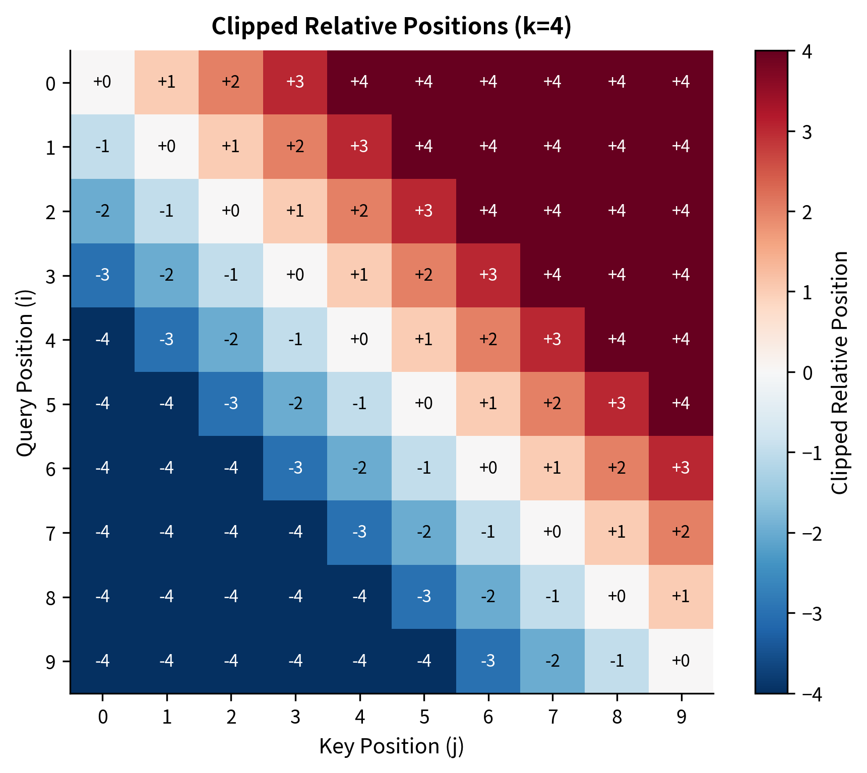
Notice the diagonal band structure: each anti-diagonal contains the same relative position. The corners, where positions are far apart, are clipped to the boundary values $\pm k$. This Toeplitz-like structure is key to efficient implementation.

Now that we understand the mathematical formulation, let's translate it into code. We'll build up the implementation in stages: first the relative position embeddings, then the modified attention score computation, then the modified value aggregation, and finally the complete layer.

The foundation of Shaw-style attention is a table of learned embeddings indexed by relative position. Since relative positions range from $-k$ to $+k$ after clipping, we need $2k + 1$ embeddings. The key implementation detail is converting from relative positions (which can be negative) to array indices (which must be non-negative).

The index conversion is the subtle but essential detail. Relative positions range from $-k$ to $+k$, but array indices must be non-negative. Adding $k$ shifts the range to $[0, 2k]$:

• Offset $-k$ (maximum backward distance) maps to index 0
• Offset 0 (same position) maps to index $k$
• Offset $+k$ (maximum forward distance) maps to index $2k$

This simple arithmetic lets us use relative positions as array indices without any conditional logic.

With the embedding table in place, we can implement the modified attention score computation. Recall the formula: $e_{ij} = (\mathbf{q}_i \cdot \mathbf{k}_j + \mathbf{q}_i \cdot \mathbf{a}^K_{j-i}) / \sqrt{d_k}$. For each query-key pair, we compute both the content term and the position term, then sum them before scaling.

This implementation iterates over all position pairs, making the logic transparent. For each pair $(i, j)$, we compute the content score ($\mathbf{q}_i \cdot \mathbf{k}_j$), look up the relative position embedding for offset $j - i$, compute the position score ($\mathbf{q}_i \cdot \mathbf{a}^K_{j-i}$), and sum them. The final division by $\sqrt{d_k}$ applies the same scaling as standard attention to prevent score magnitudes from growing with dimension.

The value aggregation follows the same pattern. For each output position $i$, we aggregate contributions from all positions $j$, but we add the relative position embedding to each value before weighting:

The value modification works similarly to the key modification. For each contributing position $j$, we add its relative position embedding $\mathbf{a}^V_{j-i}$ to its value vector before applying the attention weight. This means the output at position $i$ contains not just weighted content, but also weighted position information about where that content originated.

With both components in place, we can assemble the complete layer. This class wraps the QKV projections, relative position embeddings, and the modified attention computation into a single forward pass:

The forward pass follows the standard self-attention pattern with two modifications. After projecting input embeddings to Q, K, and V, we use our modified relative_attention_scores function instead of the standard dot product, and we use relative_attention_output instead of the standard weighted sum. The softmax step remains unchanged, as the relative position terms are already incorporated into the scores.

Let's verify our implementation produces sensible results:

The attention weights look similar to standard self-attention, but they now incorporate relative position information. Each query-key compatibility is biased by the relative distance between positions.

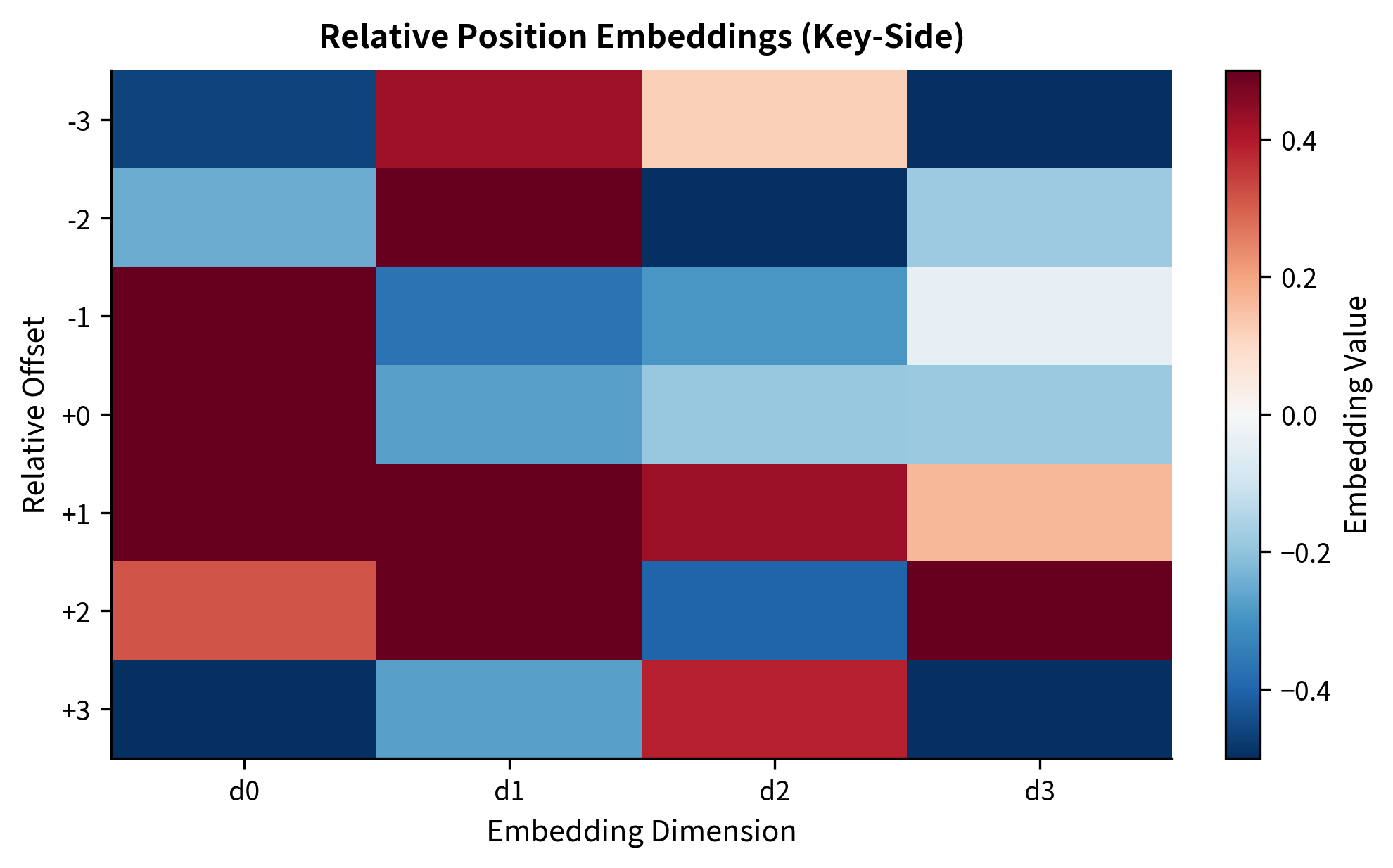
The embedding matrix shows how each relative offset is encoded as a different vector. Offset 0 (same position) has a distinct pattern from offset -3 (three positions back) or offset +3 (three positions forward). These patterns are learned during training to capture which distances are relevant for the task.

Let's visualize how relative position embeddings influence attention. We'll examine the position term $\mathbf{q}_i \cdot \mathbf{a}^K_{j-i}$ separately from the content term.

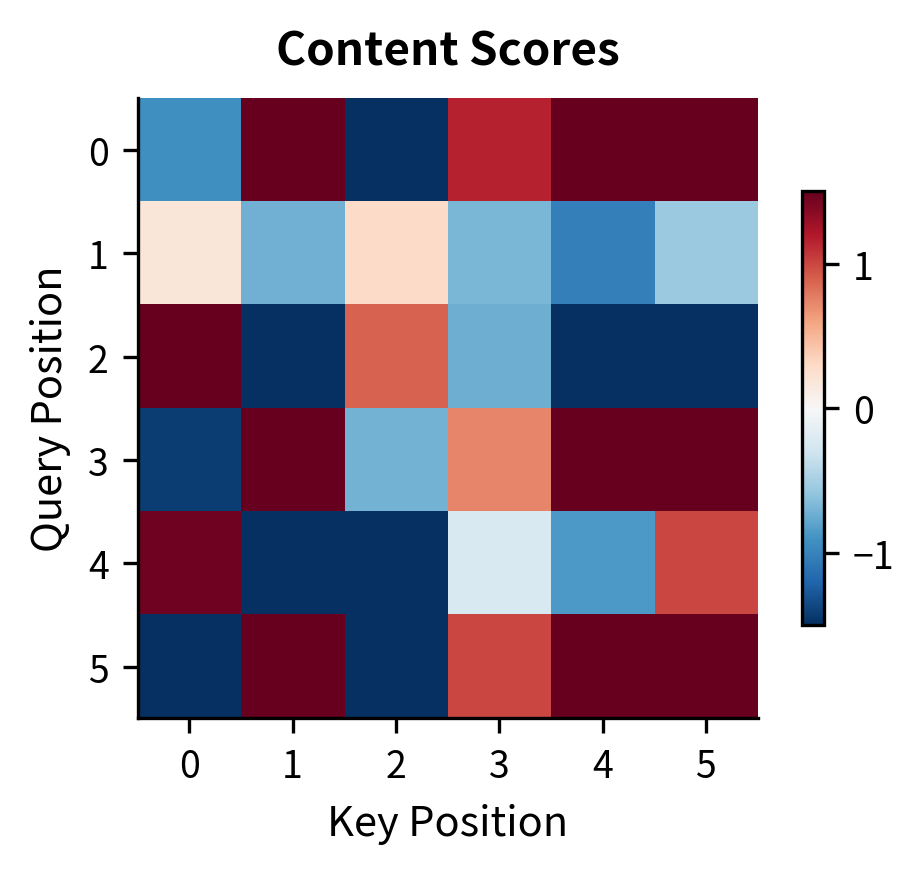
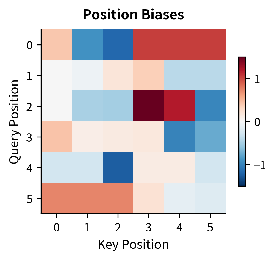
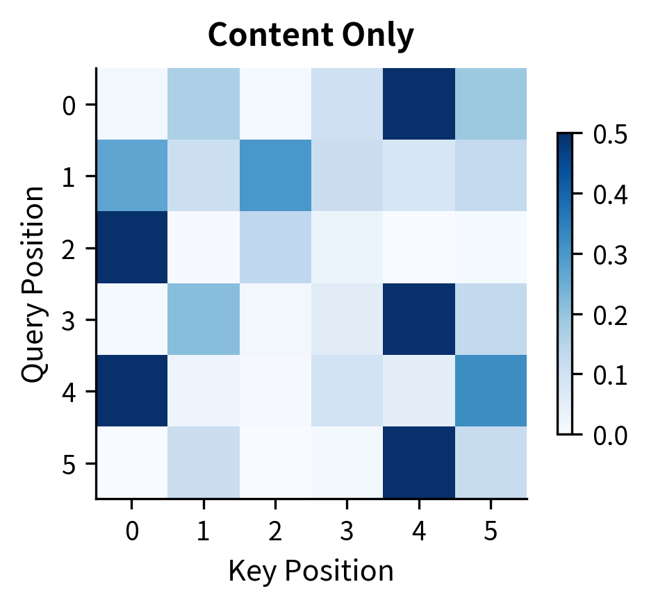
The content scores show irregular patterns depending on the input embeddings. The position biases show a distinctive diagonal structure: each anti-diagonal corresponds to positions at a fixed relative distance. For example, the main diagonal (offset 0) shows self-attention bias, while diagonals above and below show biases for looking forward and backward.

Let's examine how the combined scores compare to content-only attention:

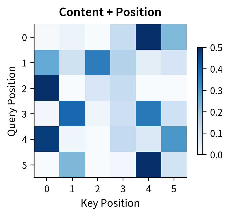
The position biases subtly shift attention patterns. In this random example, the differences are modest because the embeddings are random. In trained models, relative position embeddings learn linguistically meaningful patterns: verbs attending strongly to positions 1-2 back (typical subject distance), determiners attending 1-2 forward (to their nouns), and so on.

The loop-based implementation above is clear but slow. In practice, we compute relative attention efficiently using matrix operations. The key insight is that position biases form a Toeplitz-like structure: all entries on each diagonal share the same relative distance.

The efficient version first computes all possible query-position dot products, then indexes into this precomputed matrix. This reduces the inner loop computation from $O(d_k)$ per entry to $O(1)$, with the upfront cost of a single $(n, 2k+1)$ matrix multiplication.

Let's directly compare relative and absolute position encodings on a simple task: detecting whether a token is attending to its immediate neighbors versus distant positions.

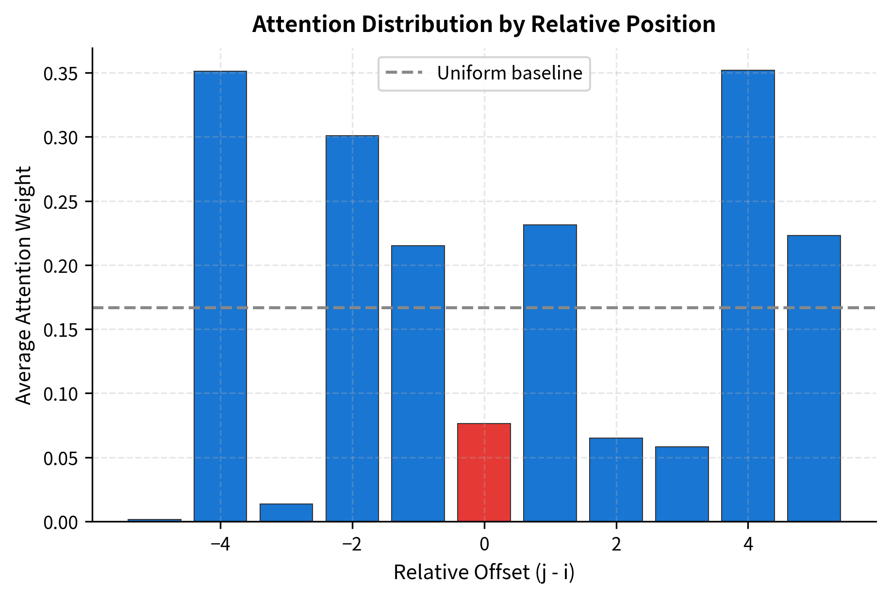
The profile shows how attention is distributed by relative distance. In this random initialization, patterns are noisy, but trained models develop clear preferences: immediate neighbors typically receive more attention, with the pattern decaying for distant positions.

To illustrate what relative position embeddings might learn, let's simulate embeddings that encode common linguistic patterns:

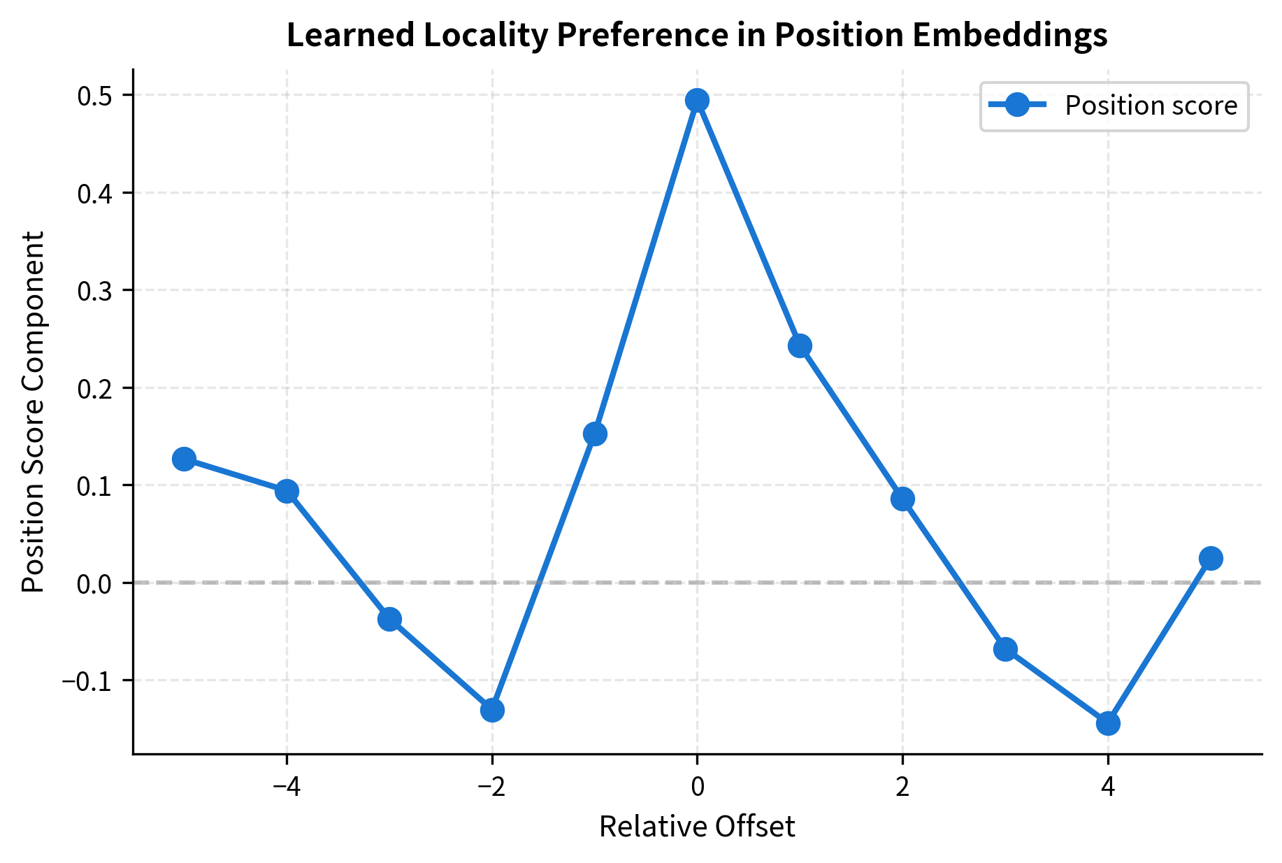
This simulated pattern shows a Gaussian-like preference for nearby positions. Real models learn more complex patterns that capture linguistic structure: determiners attending to following nouns, verbs attending to preceding subjects, and so on.

When implementing relative position encoding, several parameters control the behavior and efficiency of the mechanism:

• max_distance (k): Maximum relative position to distinguish. Positions beyond this distance share the same "far away" embedding. Typical values range from 16 to 128. Smaller values reduce memory but lose fine-grained distance information for distant positions. Larger values preserve more detail but require more parameters and training data.
• d_k: Dimension of query and key vectors (and key-side relative position embeddings). Must match between queries and keys for dot product compatibility. Common values are 64 for single-head attention or embed_dim / num_heads for multi-head attention.
• d_v: Dimension of value vectors (and value-side relative position embeddings). Determines the output dimension of each attention head. Often set equal to d_k for simplicity.
• Embedding initialization scale: Relative position embeddings are typically initialized with small random values. Xavier/Glorot initialization scales by $\sqrt{2/(n\_\text{positions} + d)}$ to maintain stable gradient magnitudes during training.

The total number of relative position parameters is $(2k + 1) \times (d_k + d_v)$. With $k = 64$ and $d_k = d_v = 64$, this adds 16,512 parameters per attention head, which is modest compared to the QKV projection matrices.

Relative position encoding solves the generalization problem but introduces its own challenges.

The most significant limitation is computational complexity. Standard absolute position encoding adds to embeddings once at the input, with no additional cost during attention. Relative position encoding modifies every attention score computation. For a sequence of length $n$, we compute $n^2$ relative position biases per attention layer. With multiple layers and attention heads, this overhead accumulates. Shaw et al. note that their approach adds roughly 5-10% to training time.

Memory usage also increases. We store $(2k+1)$ relative position embeddings per dimension, for both keys and values. With $d_k = d_v = 64$ and $k = 64$, this adds about 16K parameters per attention head. This is modest compared to the projection matrices, but still non-trivial for models with many heads.

The clipping distance $k$ introduces a hyperparameter choice. Too small, and the model loses fine-grained distance information. Too large, and distant embeddings have insufficient training signal. In practice, $k$ is often set to match the typical context length during training, such as 64 or 128 for sentence-level tasks.

Despite these limitations, relative position encoding's impact on transformer research has been substantial. It demonstrated that position information can be injected at the attention level rather than the embedding level, opening the door to more sophisticated schemes like Rotary Position Embeddings and ALiBi that we'll explore in subsequent chapters.

Relative position encoding shifts the focus from "where am I?" to "how far apart are we?" By encoding the offset between positions rather than absolute indices, models learn patterns that generalize across all positions at the same distance.

Key takeaways from this chapter:

• Absolute positions limit generalization: A model trained on short sequences may never see position pairs that appear in longer sequences. Relative encoding ensures that distance patterns transfer regardless of absolute position.

• Shaw et al. formulation: Modify attention scores by adding $\mathbf{q}_i \cdot \mathbf{a}^K_{j-i}$ to the content term. This separates semantic compatibility from distance-based compatibility.

• Clipping bounds memory: Relative positions beyond distance $k$ share the same embedding. This limits the number of parameters to $2k + 1$ regardless of sequence length.

• Two components to modify: Shaw et al. add relative embeddings to both keys (affecting which positions get attention) and values (affecting what content flows). Both contribute to the learned distance patterns.

• Diagonal structure in attention: Position biases form a Toeplitz-like pattern where each anti-diagonal corresponds to a fixed relative distance. This structure enables efficient computation.

• Trade-off between complexity and generalization: Relative position encoding adds computational overhead but provides better generalization to unseen position pairs and longer sequences.

In the next chapter, we'll explore Rotary Position Embeddings (RoPE), a method that encodes relative positions through rotation rather than additive biases. RoPE achieves similar generalization benefits with a more elegant mathematical formulation that integrates naturally with the attention computation.

Ready to test your understanding? Take this quick quiz to reinforce what you've learned about relative position encoding.