

Learn how feed-forward networks provide nonlinearity in transformers, with 2-layer architecture, 4x dimension expansion, parameter analysis, and computational cost comparisons with attention.

This article is part of the free-to-read Language AI Handbook
Choose your expertise level to adjust how many terms are explained. Beginners see more tooltips, experts see fewer to maintain reading flow. Hover over underlined terms for instant definitions.
Feed-Forward Networks
Self-attention lets tokens gather contextual information from across the sequence. But attention alone is limited: it computes weighted averages of value vectors, a fundamentally linear operation. After softmax normalization, each output position is a convex combination of value vectors. To learn complex functions of language, transformers need nonlinearity. The feed-forward network (FFN) provides exactly this, applying the same pointwise transformation to every position independently.
Every transformer block contains two main components: a self-attention sublayer and a feed-forward sublayer. While attention handles inter-token communication, the FFN handles per-token computation. This division of labor is elegant: attention routes information between positions, and the FFN transforms information at each position. Together, they enable transformers to learn rich, hierarchical representations of language.
This chapter examines the FFN in detail. You'll learn its two-layer architecture, understand why the hidden dimension is expanded, see how the computation is independent across positions, and calculate the substantial parameter count that makes FFNs the largest component of most transformer models.
The Position-Wise Feed-Forward Network
To understand why transformers need the feed-forward network, consider what attention alone provides. Self-attention computes weighted averages of value vectors, where the weights come from query-key similarities. This is powerful for gathering contextual information, but it's fundamentally a linear operation. After all the softmax normalization, each output is just a convex combination of the input representations. No matter how sophisticated the attention patterns, the function from inputs to outputs remains linear.
Linear functions have severe limitations. They can only rotate, scale, and translate the input space. They cannot learn the curved decision boundaries that separate "cat" from "car," or the complex feature interactions that distinguish sarcasm from sincerity. For a model to approximate arbitrary functions of language, it needs nonlinearity.
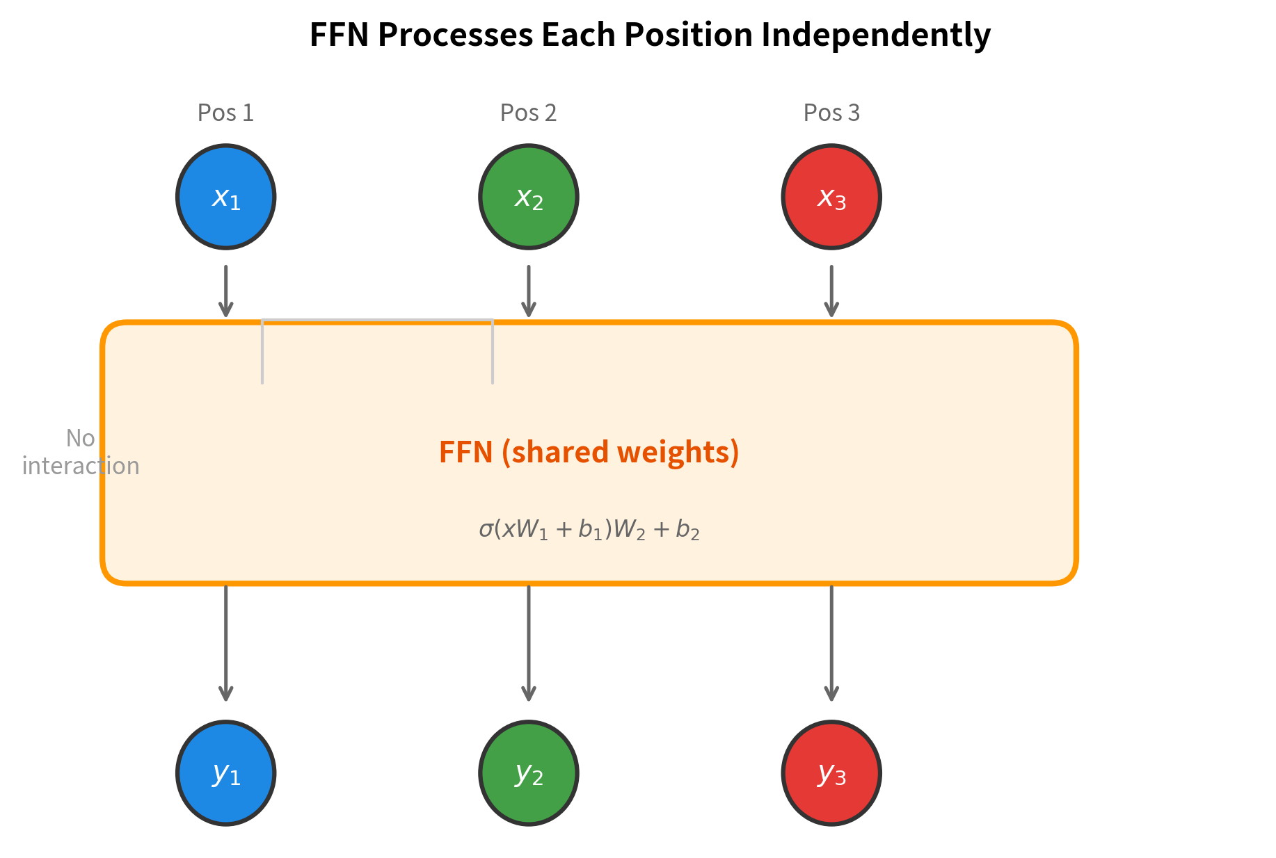
The feed-forward network (FFN) provides exactly this missing ingredient. It applies a nonlinear transformation to each token's representation, injecting the expressiveness that attention lacks. But there's a key design choice: instead of mixing information across positions like attention does, the FFN processes each position independently. If your sequence has 100 tokens, the FFN applies the same transformation to each of those 100 representations separately, using identical weights for all positions.
A position-wise operation applies the same function to each position in a sequence independently. The function's parameters are shared across positions, but the inputs and outputs at each position don't interact with each other.
This division of labor is elegant and deliberate. Attention handles inter-position communication: it routes information between tokens, allowing the model to build representations that depend on context. The FFN handles intra-position computation: it transforms each position's representation using a learned nonlinear function. By separating these concerns, the transformer achieves both contextual awareness (from attention) and expressive power (from the FFN).
Why share the same network across all positions? Two reasons justify this choice. First, language exhibits translation invariance: the grammatical patterns that help understand "the cat" are equally useful whether those words appear at the beginning, middle, or end of a sentence. A useful transformation should work wherever it's needed. Second, parameter sharing dramatically reduces model size. Instead of learning separate networks for each of the potentially thousands of positions in a sequence, we learn one network that generalizes across all positions.
The Two-Layer Architecture
With this motivation in place, let's examine what the FFN actually computes. The architecture is surprisingly simple: two linear transformations with a nonlinear activation function sandwiched between them. But this simplicity is deceptive, as we'll see, this structure enables remarkably expressive transformations.
Consider a single token's representation, a vector with dimensions. The FFN transforms this vector in three stages:
- Expand: Project into a higher-dimensional space
- Transform: Apply nonlinearity to enable learning of curved boundaries
- Contract: Project back to the original dimension
The complete formula captures all three stages in one expression:
To understand this formula, let's read it from the inside out, following the order of operations:
Stage 1: The Expansion ()
The input vector is multiplied by a weight matrix and shifted by a bias vector . This is a standard linear transformation, but with a twist: the output dimension is larger than the input dimension. If has 512 dimensions, the result might have 2048 dimensions. We're projecting into a higher-dimensional space where the data is easier to manipulate.
Stage 2: The Nonlinearity ()
The activation function is applied element-wise to the expanded representation. Common choices include ReLU (which zeros out negative values) and GELU (a smoother alternative). This is where the magic happens: the nonlinearity allows the network to learn curved decision boundaries that would be impossible with linear transformations alone.
Stage 3: The Contraction ()
Finally, the transformed representation is projected back to the original dimension via weight matrix and bias . The output has the same dimensionality as the input, which is essential for the residual connection that adds the FFN output back to its input.
Here's the complete specification of all variables:
- : the input vector for a single position (the token's representation from the previous layer)
- : the first projection matrix, which expands the dimension from to
- : the first bias vector, added after the first linear transformation
- : a nonlinear activation function (e.g., ReLU, GELU) applied element-wise to the hidden representation
- : the second projection matrix, which contracts the dimension back from to
- : the second bias vector, added to produce the final output
- : the hidden (or intermediate) dimension, typically set to
The expansion ratio is a key hyperparameter. The original transformer used a 4x expansion: for , the hidden dimension was . This ratio has become a de facto standard, though modern architectures sometimes use different values (especially when combined with gated variants, as we'll see in a later chapter).
Implementation
With the formula understood, translating it to code reveals its simplicity. The entire FFN is just two matrix multiplications with a nonlinearity in between:
The FFN preserves the dimensionality of its input: a 512-dimensional vector goes in, and a 512-dimensional vector comes out. This is essential for the residual connection that adds the FFN output back to its input.
The Hidden Dimension Expansion
The most striking aspect of the FFN architecture is the dimension expansion. The first linear layer projects from to , typically with . For a model with , this means expanding to 2048 dimensions before projecting back down.
Why expand the dimension? The answer lies in the expressiveness of the network. A fundamental result from neural network theory shows that wider hidden layers can approximate more complex functions. Consider what happens without expansion: if , the hidden layer has the same dimensionality as the input. While the formula still applies, the network has limited capacity to decompose and recombine features.
With a larger hidden dimension, the network can decompose the input into more components, transform them independently, and recombine them in complex ways. Think of it as temporarily working in a higher-dimensional space where the data is easier to manipulate, then projecting back to the original space.
The 4x expansion factor was established in the original "Attention Is All You Need" paper and has become a standard choice. Modern models like LLaMA use slightly different ratios (around 2.7x) when using gated linear units (GLUs), which effectively increase the hidden dimension through gating.
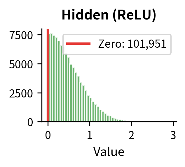
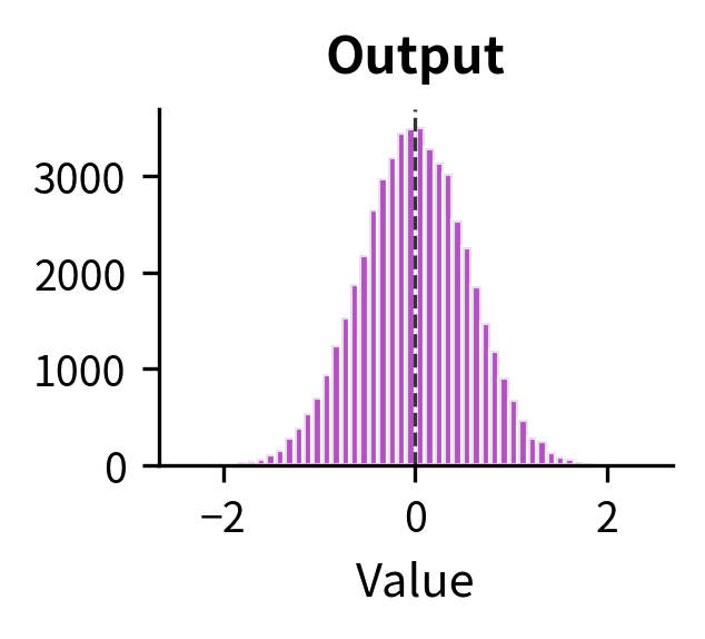
Let's visualize how the actual activation values change through each stage of the FFN:
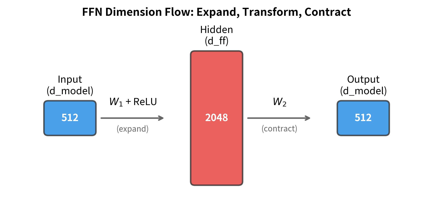
Now let's visualize the dimension sizes at each stage with a schematic:
Position Independence
A critical property of the FFN is that it processes each position independently. Unlike attention, where every position can influence every other position, the FFN applies an identical transformation to each position in isolation. This has important implications for both computation and interpretation.
Let's verify this independence empirically:
The batch and individual processing produce identical results (up to floating-point precision). This confirms that positions don't interact within the FFN.
Why is this important? Position independence means the FFN can be computed in parallel across all positions. On a GPU, this is extremely efficient: instead of processing tokens sequentially, we process the entire sequence simultaneously. The FFN is embarrassingly parallel.
Position independence also clarifies the division of labor in a transformer block. Attention handles inter-position communication: it routes information between tokens, allowing the model to build representations that depend on context. The FFN handles intra-position transformation: it transforms each position's representation using the same learned function, adding nonlinearity and processing capacity to what would otherwise be a purely linear attention mechanism.
Interpreting the FFN as Key-Value Memory
Recent research has revealed a fascinating interpretation of feed-forward layers: they function as associative memories, storing key-value pairs in their weights. This perspective, developed by researchers at Tel Aviv University and other institutions, helps explain how transformers store and retrieve factual knowledge.
The idea is elegant. Consider the first layer's weight matrix . Each column of (which we can denote as for the -th column) can be thought of as a "key" that matches certain input patterns. The pre-activation for hidden dimension is computed as:
where:
- : the pre-activation value for hidden dimension
- : the input vector (-dimensional)
- : the -th column of , acting as a "key" pattern
- : the -th element of the bias vector
When the input aligns well with key (high dot product), the corresponding hidden dimension activates strongly. After ReLU, only positive activations survive.
The second layer's weight matrix contains the "values" associated with each key. Each row of (denoted for the -th row) is the value vector that gets added to the output when hidden dimension is active. The final output is a weighted sum of these values, where the weights are the hidden activations.
The feed-forward layer can be interpreted as an associative memory where columns are keys, hidden activations are match scores, and rows are values. Input patterns that match certain keys retrieve their associated values.
Let's visualize this interpretation:
Let's visualize this sparsity pattern across multiple inputs to see how different inputs activate different subsets of hidden dimensions:
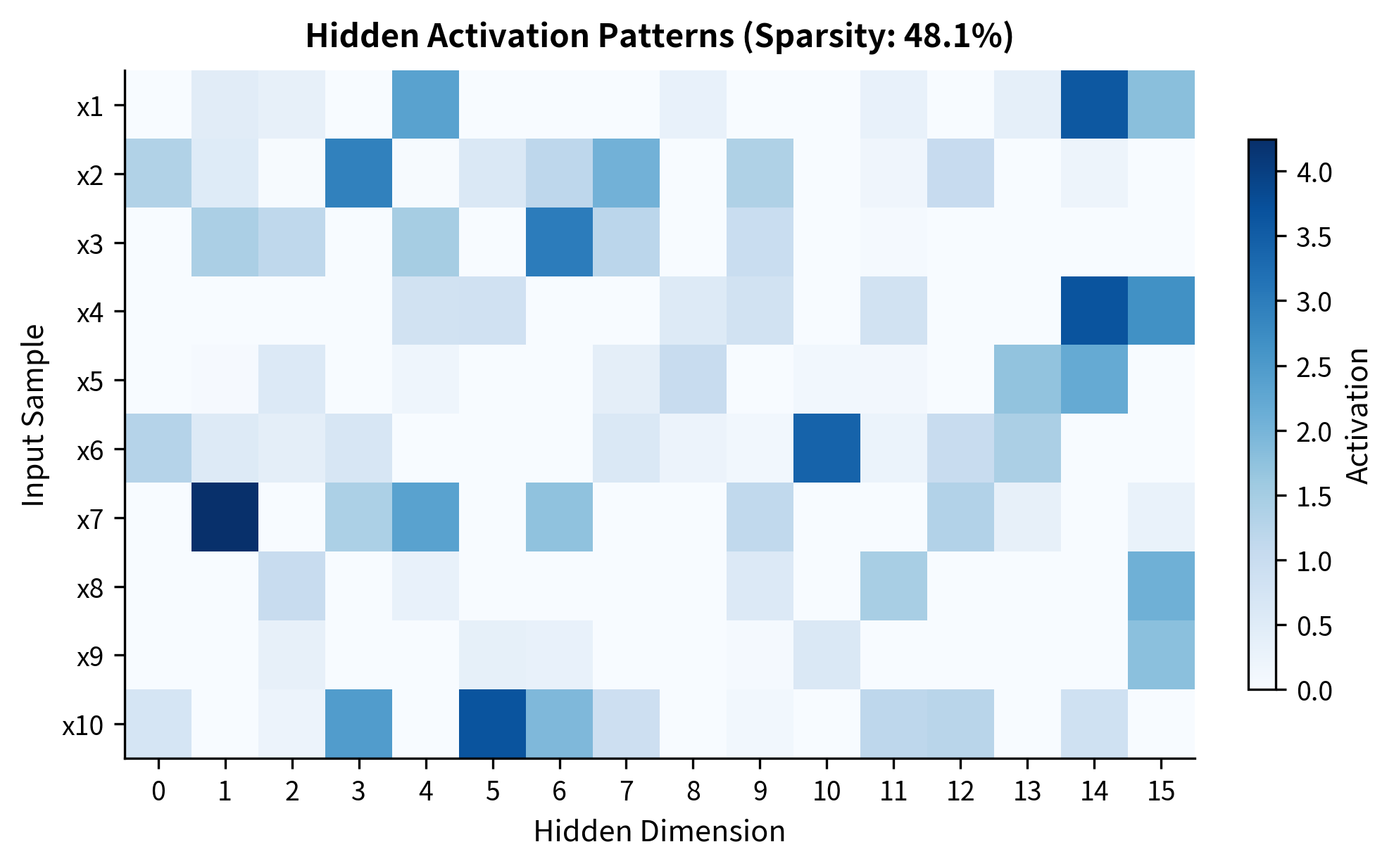
This memory interpretation explains several empirical observations about transformers. Researchers have found that specific neurons in FFN layers activate for particular concepts: there are neurons that activate for "the Eiffel Tower," "programming languages," or "past tense verbs." These neurons encode factual associations in their weights, and the FFN retrieves them when relevant patterns appear in the input.
Parameter Count Analysis
Feed-forward networks are the largest component of transformer models by parameter count. In a standard transformer, the FFN contains significantly more parameters than the attention mechanism. Understanding this is crucial for model scaling and efficiency optimization.
For a single FFN layer, we can count the total number of learnable parameters by summing the sizes of all weight matrices and bias vectors:
where:
- : the number of parameters in weight matrix (first term contributes this once)
- : the number of parameters in weight matrix (note: has the same total count as , just transposed dimensions)
- : the number of parameters in bias vector
- : the number of parameters in bias vector
The factor of 2 in front of accounts for both weight matrices and .
With the standard expansion factor , we can simplify this expression. Substituting:
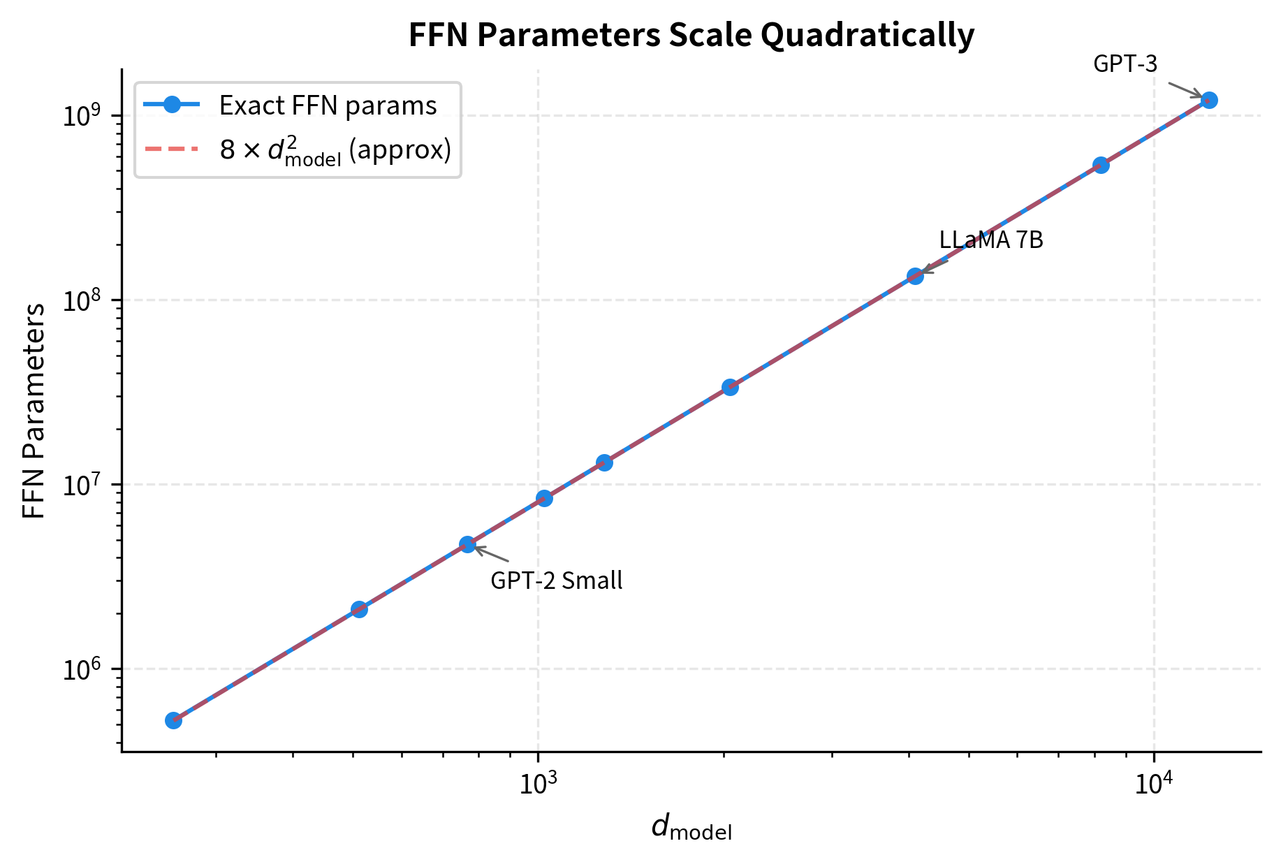
For large models where is in the hundreds or thousands, the quadratic term dominates and the linear bias terms become negligible, giving approximately parameters per FFN layer.
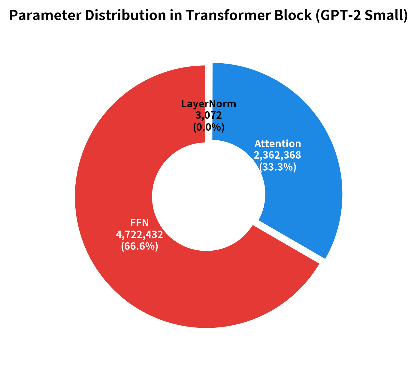
The FFN consistently contains about twice as many parameters as the attention mechanism per layer. For large models like GPT-3, each transformer layer has over 2.4 billion parameters in the FFN alone. This makes FFN optimization critical for model efficiency.
Let's visualize how FFN parameters scale with model dimension:
Let's also visualize the parameter distribution in a transformer block:
Computational Cost
Beyond parameter count, we should consider computational cost, measured in floating-point operations (FLOPs). Understanding FFN compute requirements helps explain why these layers dominate inference time for short sequences.
For each token, the FFN performs two matrix-vector multiplications:
- First layer: Computing (where is a -dimensional vector and is ) requires multiply-add operations
- Second layer: Computing (where is a -dimensional hidden vector and is ) requires multiply-add operations
Each multiply-add consists of one multiplication and one addition, so it counts as 2 floating-point operations. The total FLOPs per token for the FFN is:
where:
- : the input and output dimension of the FFN
- : the hidden dimension (typically )
- The factor of 4 comes from: 2 layers 2 operations per multiply-add
For a sequence of tokens, each token is processed independently, so the total FFN cost scales linearly with sequence length:
where is the number of tokens in the sequence.
This linear scaling contrasts sharply with attention, which has quadratic complexity due to the attention matrix computation. As sequences grow longer, attention's quadratic term eventually dominates.
For short sequences, the FFN dominates computational cost (due to its large weight matrices). As sequences grow longer, attention's quadratic complexity catches up. At around 1024-2048 tokens, attention and FFN have comparable costs. Beyond that, attention becomes the bottleneck.
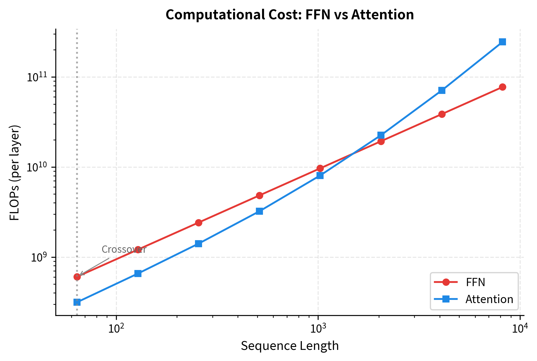
This crossover point explains why long-context models focus heavily on attention efficiency (sparse attention, linear attention, etc.) while short-context applications often emphasize FFN optimization (quantization, pruning).
A Complete Worked Example
The formula is compact, but its compactness can obscure what's actually happening. To truly understand the FFN, let's trace through a concrete computation with actual numbers. We'll use intentionally small dimensions, and , so you can follow every multiplication and addition by hand.
The goal of this example is threefold: (1) see exactly how the input vector is transformed at each stage, (2) observe how ReLU zeros out negative activations to introduce nonlinearity, and (3) verify that the output dimension matches the input dimension, ready for the residual connection.
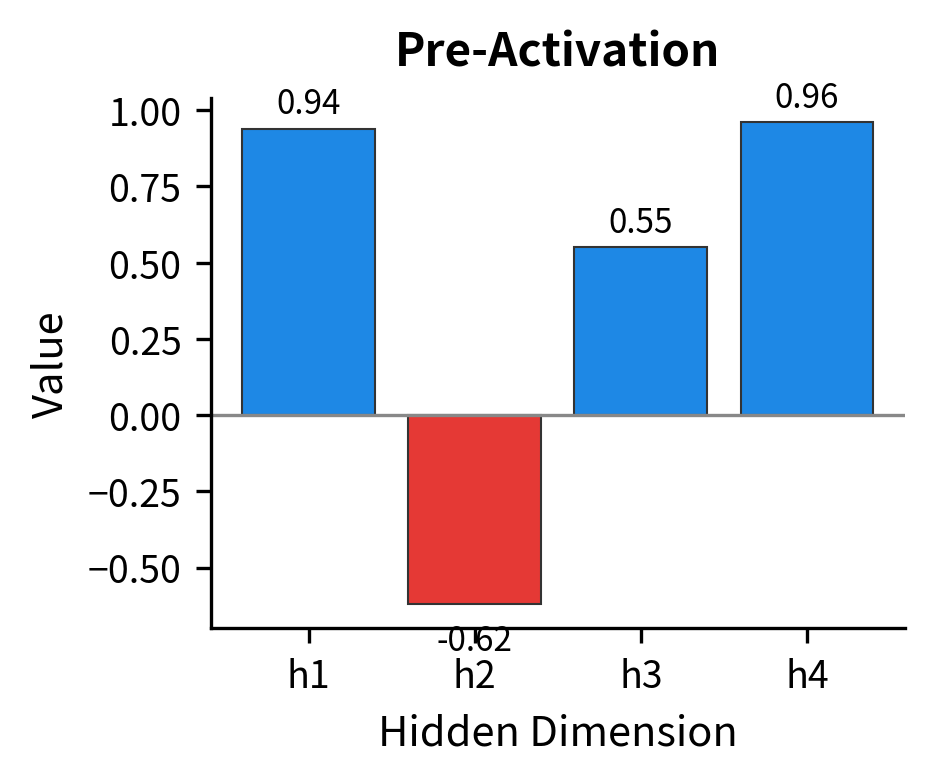
Stage 1: Expansion via the First Linear Layer
The first operation computes . Our 3-dimensional input vector gets multiplied by a weight matrix, producing a 4-dimensional hidden representation. Each element of this output is a weighted sum of the input elements plus a bias term.
Notice the dimension change: a 3-dimensional vector goes in, a 4-dimensional vector comes out. This expansion is the "higher-dimensional space" we discussed earlier, where the network has more room to manipulate the representation. The result is called the pre-activation because we haven't applied the nonlinearity yet.
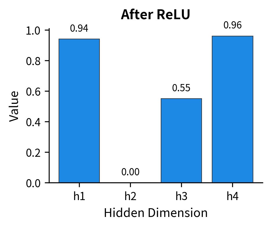
Stage 2: Nonlinearity via ReLU
Here's where the FFN gains its expressive power. The ReLU activation function applies a simple rule: keep positive values unchanged, but set negative values to zero. Mathematically, .
This seemingly simple operation has profound consequences. By zeroing out some dimensions, ReLU creates sparse hidden representations, meaning only a subset of hidden dimensions are active for any given input. Different inputs activate different subsets, allowing the network to learn piece-wise linear functions that approximate arbitrary curves. This is the source of the FFN's nonlinear expressive power.
Stage 3: Contraction via the Second Linear Layer
Finally, we project back to the original dimension. The 4-dimensional hidden vector is multiplied by a weight matrix, and a 3-dimensional bias is added.
The output has the same dimension as the input, exactly 3 elements. This is essential: in the full transformer, this output will be added to the original input via a residual connection, and both must have the same shape.
Verification and Summary
Let's verify that our step-by-step calculation matches the complete FFN function, and summarize what we've learned:
The step-by-step and function-based computations match exactly. This worked example demonstrates the complete journey: a 3-dimensional input expands to 4 dimensions, passes through nonlinearity (with some dimensions zeroed out), and contracts back to 3 dimensions. The FFN has transformed the input representation while preserving its dimensionality, exactly as the formula describes.
Implementation: A Complete FFN Module
Having traced through the mathematics by hand, we can now build a reusable FFN module that encapsulates everything we've learned. This implementation follows patterns used in production transformer libraries: it initializes weights using proper scaling (Xavier/Glorot initialization), supports optional biases, and handles both single vectors and batched sequences.
Limitations and Impact
The feed-forward network is conceptually simple: two linear layers with a nonlinearity in between. Yet this simplicity masks significant computational cost. The FFN accounts for roughly two-thirds of a transformer block's parameters and dominates compute for short sequences. This has driven extensive research into FFN efficiency.
Sparsity offers one path forward. The ReLU activation naturally creates sparse hidden representations, as negative pre-activations become zero. Researchers have exploited this by identifying which hidden dimensions will be active for a given input and computing only those, skipping computation for dimensions that would be zeroed anyway. The Mixture of Experts (MoE) architecture takes this further, replacing the single FFN with multiple "expert" FFNs and routing each token to only a subset of experts. This allows models to scale parameters without proportionally scaling compute.
Quantization provides another avenue for efficiency. Since FFN weights are static after training, they can be compressed to lower precision (8-bit, 4-bit, or even 2-bit integers) with careful calibration. This reduces memory bandwidth, often the bottleneck in FFN computation, and enables faster inference.
Despite its computational weight, the FFN's role is essential. It provides the nonlinearity that transforms attention's linear weighted averages into expressive function approximation. It serves as the model's "memory," storing factual associations in its weights that attention retrieves based on context. And its position-wise nature enables massive parallelization that makes transformer training tractable.
The interplay between attention and FFN defines transformer expressiveness. Attention routes information between positions, creating context-dependent representations. The FFN transforms those representations position-by-position, adding computational depth. Together, they enable the hierarchical, compositional language understanding that powers modern NLP.
Summary
The feed-forward network is the workhorse of transformer computation, applying identical transformations to each position independently. This chapter explored its architecture, efficiency characteristics, and role in the broader transformer block.
Key takeaways:
-
Two-layer architecture: The FFN formula consists of an expansion layer (), a nonlinear activation (ReLU, GELU, etc.), and a contraction layer (). The standard expansion factor is .
-
Position independence: Each position is processed separately with shared weights. This enables parallel computation and separates the FFN's role (per-position transformation) from attention's role (inter-position communication).
-
Key-value memory interpretation: The FFN can be viewed as an associative memory where columns are keys, hidden activations are match scores, and rows are values. This explains how transformers store factual knowledge.
-
Dominant parameter count: The FFN contains approximately two-thirds of a transformer block's parameters. With 4x expansion, the total is approximately parameters per layer (from the formula ). This makes FFN optimization critical for model efficiency.
-
Linear computational scaling: FFN compute cost is FLOPs, scaling linearly with sequence length . This contrasts with attention's quadratic scaling. For short sequences, FFN dominates compute; for long sequences, attention becomes the bottleneck.
-
Crossover point: Around 1000-2000 tokens, FFN and attention have comparable computational costs. This crossover influences optimization strategies for different sequence lengths.
The next chapter examines activation functions used in FFNs, comparing ReLU, GELU, SiLU/Swish, and understanding why modern models have moved beyond the original ReLU choice.
Key Parameters
When implementing or configuring feed-forward networks in transformers, these parameters control capacity and efficiency:
-
d_model (input/output dimension): The embedding dimension that the FFN preserves. Typical values range from 256 (small models) to 12288 (GPT-3 scale). This dimension must match the attention layer output and determines the FFN's interface with the rest of the transformer.
-
d_ff (hidden dimension): The expanded dimension of the intermediate representation. The standard choice is , though modern architectures like LLaMA use ratios around 2.7x when combined with gated linear units. Larger values increase expressiveness but proportionally increase parameters and compute.
-
activation: The nonlinear function applied element-wise after the first linear layer. ReLU was used in the original transformer, but GELU has become the standard for encoder models (BERT, RoBERTa) and SiLU/Swish for decoder models (LLaMA, GPT-NeoX). The choice affects gradient flow and sparsity patterns.
-
use_bias: Whether to include bias terms and . Some modern architectures (LLaMA, PaLM) omit biases entirely to reduce parameters and simplify quantization. The impact on model quality is typically minimal.
-
dropout (not shown in our implementation): Dropout rate applied to the hidden representation after activation. Values of 0.1-0.2 are common during training to prevent overfitting. Set to 0 during inference.
-
initialization: Weight initialization scale affects training stability. Xavier/Glorot initialization (scaling by ) is standard. Some architectures use scaled initialization for residual paths to maintain signal magnitude through deep networks.
Quiz
Ready to test your understanding? Take this quick quiz to reinforce what you've learned about feed-forward networks in transformers.

Comments