

Complete guide to BERT pre-training covering masked language modeling, next sentence prediction, data preparation, hyperparameters, and training dynamics with code implementations.

This article is part of the free-to-read Language AI Handbook
Choose your expertise level to adjust how many terms are explained. Beginners see more tooltips, experts see fewer to maintain reading flow. Hover over underlined terms for instant definitions.
BERT Pre-training
Pre-training is where BERT learns language. Starting from random weights, the model processes billions of words and emerges with representations that capture syntax, semantics, and even world knowledge. This transformation happens through two complementary objectives: predicting masked tokens and recognizing whether sentences belong together.
Understanding BERT's pre-training reveals why it works so well. The training data, masking strategies, auxiliary objectives, and hyperparameters all interact to produce a model that transfers effectively to downstream tasks. This chapter walks through each component: how the data is prepared, how the objectives shape learning, what hyperparameters matter, and how long training takes to converge.
Pre-training Data
BERT's knowledge comes from text. The original model trained on two massive corpora: the BooksCorpus and English Wikipedia. Together, these sources provide around 3.3 billion words of diverse, high-quality text.
A collection of approximately 11,000 unpublished books spanning multiple genres, totaling around 800 million words. Originally compiled for book-to-movie alignment research, it provides long-form narrative text with coherent multi-sentence structure.
The BooksCorpus contributes long-form narrative text with coherent story structure. Each book maintains consistent style, character references, and thematic development across thousands of sentences. This teaches the model long-range dependencies that isolated sentences cannot provide.
Wikipedia adds encyclopedic knowledge. Its articles cover history, science, geography, biography, and countless specialized domains. The text is well-edited, factually dense, and structurally organized with clear section boundaries. From Wikipedia, BERT learns factual associations, entity relationships, and formal writing conventions.
The combination matters. Fiction teaches narrative flow, dialogue patterns, and emotional language. Non-fiction teaches factual structure, technical vocabulary, and logical argumentation. Together, they produce representations that generalize across domains.
Document Structure
Pre-training data must preserve document boundaries because one of BERT's objectives requires sampling sentence pairs from the same document. Each document is processed as a sequence of sentences, maintaining the original order.
The data pipeline typically proceeds as follows:
- Document collection: Gather raw text organized by document (books, articles, pages)
- Sentence segmentation: Split documents into individual sentences using punctuation and linguistic rules
- Tokenization: Convert sentences to WordPiece token sequences
- Pair construction: Create training examples by combining sentence pairs
For Wikipedia, each article forms a document. For BooksCorpus, each book forms a document. Sentence boundaries are detected using simple heuristics (periods followed by spaces and capital letters) combined with special handling for abbreviations and quotations.
Real preprocessing pipelines handle edge cases like abbreviations ("Dr.", "U.S."), URLs, quotations, and numbered lists. BERT's original preprocessing used a combination of sentence boundary detection libraries and manual filtering.
Creating Training Examples
Each training example for BERT consists of two segments (which we call sentence A and sentence B) joined with special tokens. The format is:
[CLS] sentence A tokens [SEP] sentence B tokens [SEP]
where [CLS] is a special classification token and [SEP] marks segment boundaries.
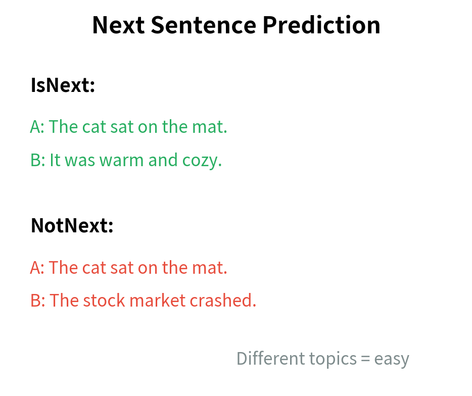
The two sentences are drawn from the same document. Half the time, sentence B immediately follows sentence A in the original text (a "positive" pair). Half the time, sentence B is a random sentence from a different location in the corpus (a "negative" pair). This sampling strategy creates the data for the Next Sentence Prediction task.
The example shows how the sampling works. Consecutive sentence pairs teach the model about discourse coherence. Random pairs teach it to distinguish coherent text from jumbled fragments. This binary classification signal, combined with masked token prediction, gives BERT a richer understanding than masking alone would provide.
Sequence Length and Packing
BERT processes fixed-length sequences, typically 512 tokens. Most sentence pairs are shorter than this limit, so multiple pairs can be packed into a single sequence to maximize GPU utilization.
The packing strategy concatenates sentence pairs until the sequence reaches the maximum length:
[CLS] pair1_A [SEP] pair1_B [SEP] [CLS] pair2_A [SEP] pair2_B [SEP] ...
However, the original BERT paper uses a simpler approach: each training example contains exactly one sentence pair, padded to the maximum length. This wastes some compute on padding tokens but simplifies the training pipeline.
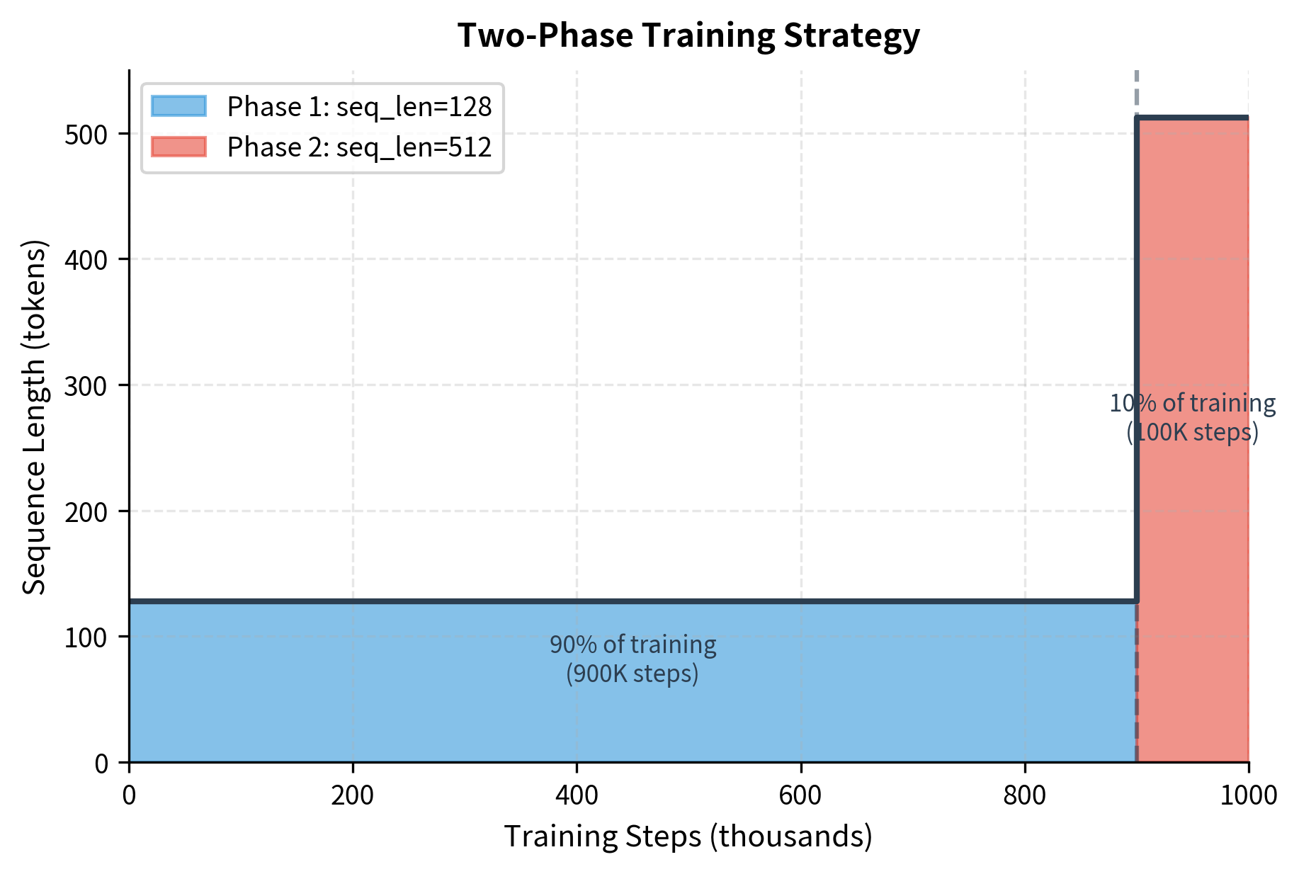
A compromise used in the original BERT paper is to sample 90% of training examples with short sequences (128 tokens) and 10% with the full length (512 tokens). Short sequences speed up initial training when the model is learning basic patterns, while long sequences in the final phase provide the context needed for complex relationships.
The MLM Objective in Practice
We covered masked language modeling conceptually in the previous chapter. Here we see exactly how BERT applies it during pre-training.
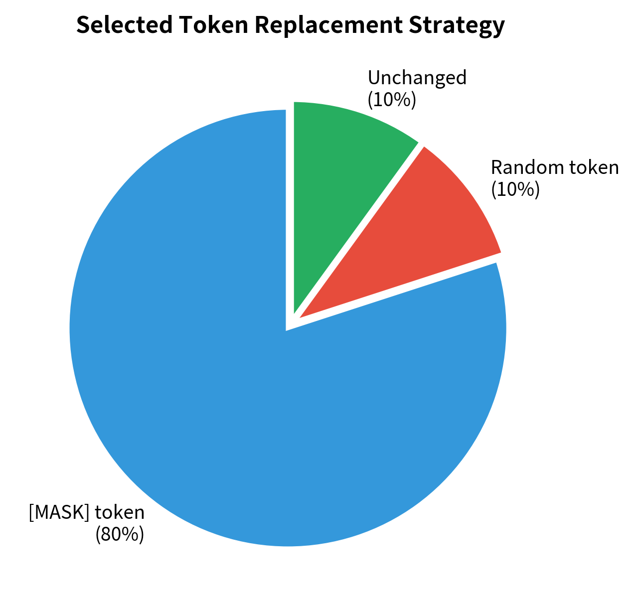
For each training sequence, BERT randomly selects 15% of tokens for prediction. Of these selected tokens:
- 80% are replaced with the
[MASK]token - 10% are replaced with a random vocabulary token
- 10% are left unchanged
The model must predict the original token at all selected positions, regardless of how they were corrupted.
The output shows which tokens were selected for masking and how each was treated. Positions with "ignore" labels don't contribute to the MLM loss. The model learns from the positions that do have labels, whether they show [MASK], a random token, or the original token.
Whole Word Masking
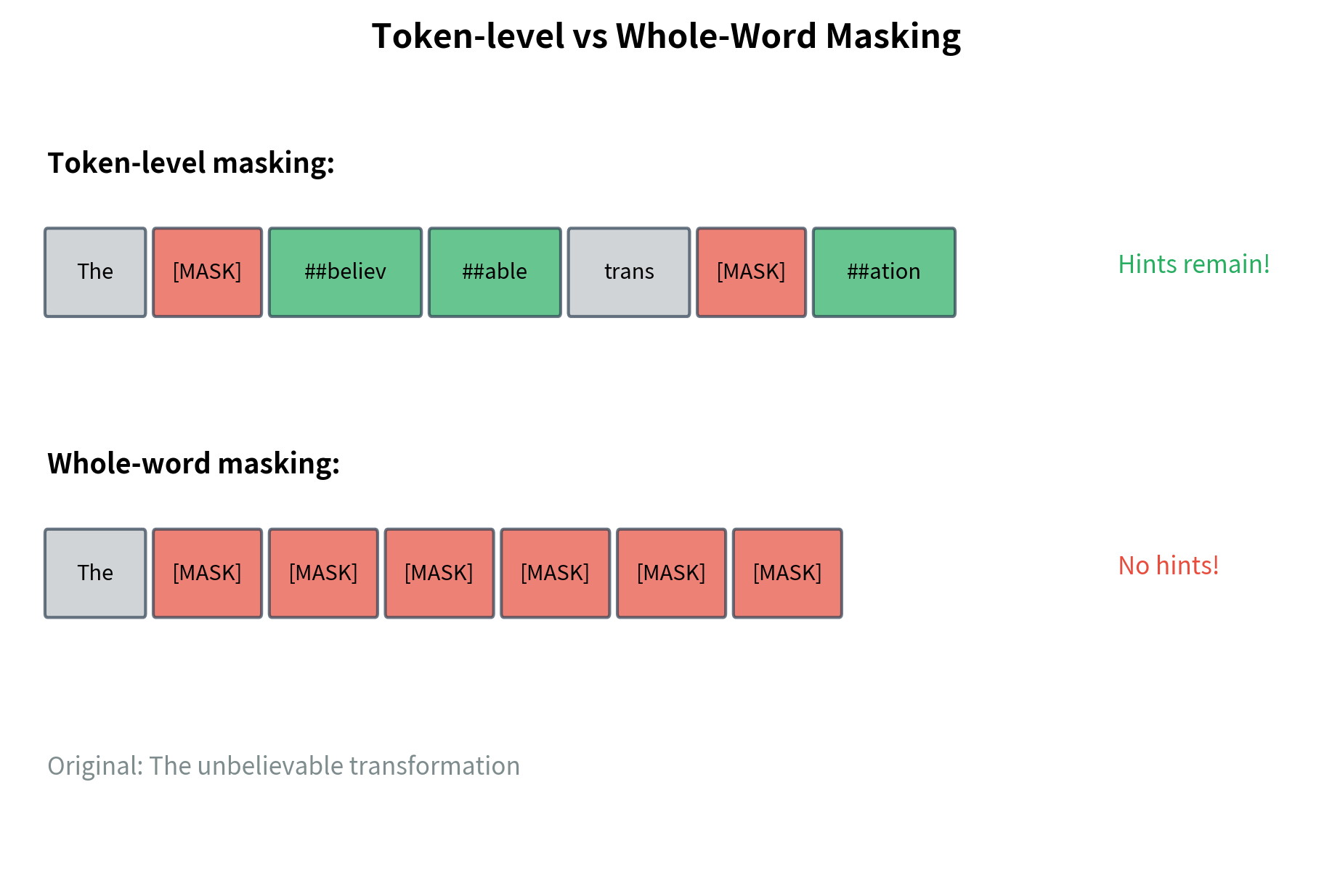
The original BERT masked individual WordPiece tokens. This created a problem: when a word like "playing" tokenizes to ["play", "##ing"], masking only "##ing" gives the model an easy hint.
BERT later adopted whole word masking (WWM), where all tokens from the same word are masked together. This provides a stronger learning signal because the model cannot peek at sibling tokens.
Notice how multi-token words get fully masked. The model cannot see any part of the word "unbelievable" or "transformation" if they are selected for masking. This produces more robust representations than token-level masking.
Next Sentence Prediction
Masked language modeling teaches BERT about word-level and sentence-level patterns. But understanding full documents requires reasoning about how sentences relate to each other. Does this sentence follow logically from the previous one? Are these two sentences from the same document?
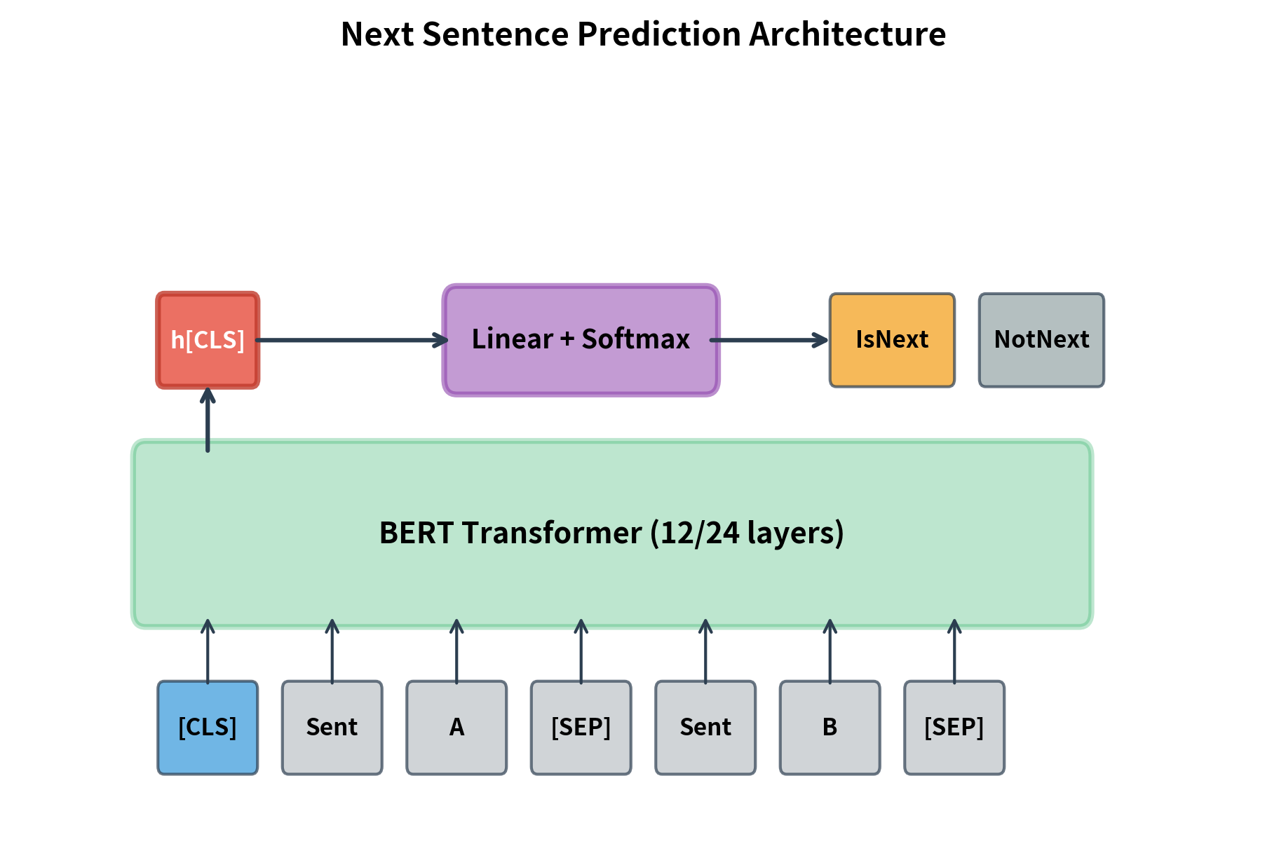
Next Sentence Prediction (NSP) provides this document-level signal. Given two sentences A and B, the model must predict whether B immediately follows A in the original corpus.
A binary classification task where the model predicts whether sentence B is the actual next sentence after sentence A in the source document (IsNext) or a random sentence from elsewhere in the corpus (NotNext).
How NSP Works
The [CLS] token's representation at the final layer is used for the NSP prediction. A small classification head (typically a single linear layer) maps this representation to two logits, one for IsNext and one for NotNext.
The training procedure constructs balanced batches with 50% positive (actual next sentence) and 50% negative (random sentence) pairs. The NSP loss is cross-entropy between the predicted probabilities and the binary label.
The NSP Controversy
NSP was designed to help BERT understand document structure, particularly for tasks like question answering where reasoning across sentences matters. However, subsequent research questioned its value.
RoBERTa (2019) found that removing NSP entirely and training on longer contiguous sequences actually improved performance. The researchers hypothesized that NSP's negative examples (random sentences from different documents) were too easy to distinguish, providing weak signal. Topic differences between sentences gave obvious cues without requiring deeper understanding.
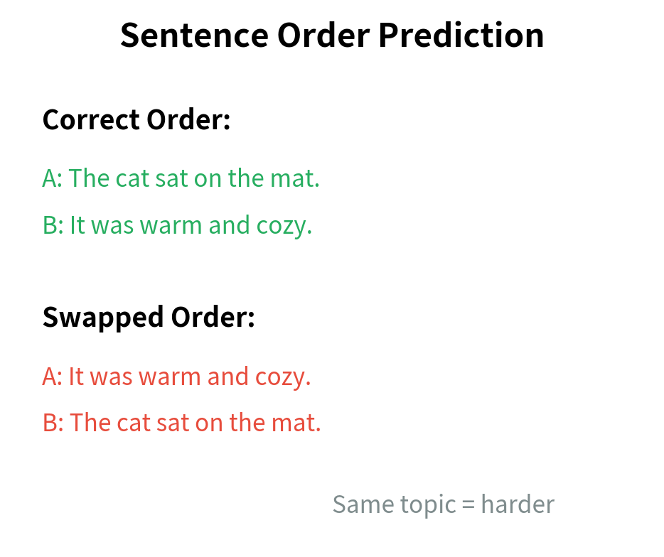
ALBERT took a different approach, replacing NSP with Sentence Order Prediction (SOP). Instead of distinguishing consecutive sentences from random ones, SOP asks whether two consecutive sentences are in the correct order or swapped. This harder task forced the model to learn finer-grained discourse relationships.
Despite the controversy, understanding NSP matters for working with pre-trained BERT models. Many available checkpoints were trained with NSP, and the [CLS] token was optimized for this task. When fine-tuning for classification, you're building on representations shaped by both MLM and NSP.
Implementing NSP
Let's implement a complete NSP training step to see how the pieces fit together:
The token_type_ids distinguish sentence A (0) from sentence B (1). This helps the model understand which tokens belong to which segment, enabling it to reason about sentence relationships.
Combined Pre-training Objective
So far we've examined BERT's two objectives separately: MLM teaches the model to understand words in context, while NSP teaches it to recognize document-level coherence. But how do these objectives work together during training? The answer lies in how we combine their signals into a single optimization target.
Why Combine Two Objectives?
Consider what each objective teaches in isolation. MLM forces the model to build rich token representations by predicting masked words from surrounding context. A model that excels at MLM understands syntax, semantics, and even factual knowledge encoded in word patterns. However, MLM operates at the sentence level. It doesn't explicitly teach the model whether two sentences belong together or flow logically from one to the other.
NSP addresses this gap. By asking "does sentence B follow sentence A?", the model must develop representations that capture discourse relationships, topic coherence, and logical flow. The [CLS] token becomes a summary of the entire sentence pair, encoding whether they form a coherent unit.
Training on both objectives simultaneously allows the model to develop representations that are rich at multiple levels: tokens capture local meaning, while the [CLS] token captures global coherence. The question becomes: how do we combine these two learning signals?
The Combined Loss Formula
BERT uses the simplest possible combination: add the losses together. Each batch of training data produces two loss values, and the total loss is their sum:
where:
- : the total pre-training loss that BERT minimizes through gradient descent
- : the masked language modeling loss, measuring how well the model predicts masked tokens
- : the next sentence prediction loss, measuring how well the model classifies sentence pairs
This equal weighting (1.0 for each) means both objectives contribute equally to the gradient updates. The model cannot cheat by ignoring one task to optimize the other. It must find parameters that satisfy both constraints simultaneously.
Understanding the MLM Loss Component
The MLM loss measures how surprised the model is by the correct answers at masked positions. If the model confidently predicts the right token, the loss is low. If it assigns low probability to the correct token, the loss is high.
Mathematically, we sum the negative log-probabilities across all masked positions:
Let's unpack each component:
- : the set of masked position indices. For a 512-token sequence with 15% masking, this contains approximately 77 positions.
- : the original token at position before we corrupted it. This is the "ground truth" the model must recover.
- : the corrupted input sequence where masked positions show
[MASK], random tokens, or unchanged tokens (following the 80-10-10 rule). - : the probability our model (with parameters ) assigns to the correct token , given the entire corrupted sequence as context.
The negative sign and logarithm work together to create our loss function. When is close to 1 (confident and correct), , contributing zero loss. When is small (the model missed the answer), becomes a large negative value, and the negative sign makes it a large positive loss. This asymmetry creates strong gradients that push the model to assign high probability to correct tokens.
Understanding the NSP Loss Component
The NSP loss has a simpler structure because it's a binary classification problem. The model looks at the [CLS] token's representation and must decide: IsNext or NotNext?
Here's what each symbol means:
- : the true binary label. We encode IsNext as 1 and NotNext as 0. This comes from how we constructed the training data (50% consecutive pairs, 50% random pairs).
- : the hidden representation of the
[CLS]token after passing through all transformer layers. This 768-dimensional vector (for BERT-base) summarizes the entire sentence pair. - : the probability the model assigns to the correct label, computed by passing through the NSP classification head.
The structure mirrors the MLM loss: negative log-probability of the correct answer. When the model confidently predicts the right class, loss is near zero. When it's wrong or uncertain, loss increases.
How the Losses Interact
Both losses share the same transformer backbone. When we compute the gradient of , it flows back through both the MLM head and the NSP head, then merges in the transformer layers. This means every transformer layer receives gradient signal from both objectives.
The interplay teaches complementary skills:
-
Token embeddings learn to represent individual words in ways that support both masked token prediction (MLM) and sentence-pair understanding (NSP).
-
Attention patterns develop to capture both local dependencies (which tokens help predict a masked word) and global coherence (what makes two sentences related).
-
The
[CLS]token becomes especially important for NSP, learning to aggregate sentence-level meaning, while other positions focus more on token-level prediction.
This multi-task learning is why BERT's representations transfer so well to diverse downstream tasks. The model has learned to encode information at multiple levels of abstraction.
Implementing the Combined Loss
Let's translate these formulas into code. PyTorch's cross_entropy function computes exactly the negative log-probability we described, making the implementation straightforward. The key insight is handling the MLM labels: we use -100 for positions that weren't masked, and PyTorch's ignore_index parameter automatically excludes these from the loss calculation.
The mlm_logits.view(-1, vocab_size) reshapes the predictions from a 3D tensor (batch, sequence, vocabulary) into a 2D tensor (batch × sequence, vocabulary). This flattening allows us to treat each position independently, which matches our formula where we sum over individual masked positions.
Now let's see what the losses look like at initialization, before any training has occurred. We'll create random logits (simulating an untrained model) and random labels (simulating our training data):
The results confirm our understanding of the loss functions. An untrained model assigns roughly uniform probability across all tokens, so the expected MLM loss is , representing maximum uncertainty over the vocabulary. Similarly, random binary classification yields expected loss . The actual values fluctuate slightly due to random sampling, but they hover around these theoretical baselines.
As training progresses, both losses decrease. The MLM loss drops as the model learns which tokens fit in which contexts. The NSP loss drops as the model learns to distinguish coherent sentence pairs from random ones. The total loss, being their sum, tracks the model's overall progress toward understanding language.
Pre-training Hyperparameters
BERT's pre-training configuration was carefully tuned. The hyperparameters balance training stability, convergence speed, and final model quality.
Optimizer Settings
BERT uses AdamW, a variant of Adam that decouples weight decay from the gradient update:
- Learning rate: Peak of 1e-4 for both BERT-base and BERT-large
- Warmup steps: 10,000 steps of linear warmup from 0 to peak learning rate
- Learning rate schedule: Linear decay from peak to 0 over the remaining training
- Weight decay: 0.01 applied to all parameters except biases and LayerNorm
- Adam : 0.9
- Adam : 0.999
- Adam : 1e-6
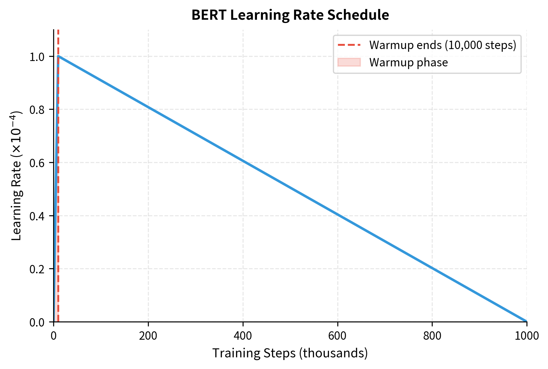
The warmup phase is critical for training stability. At initialization, gradients can be very large. Starting with a high learning rate would cause the model to diverge. Warmup gradually increases the learning rate, allowing the model to find a reasonable parameter region before taking larger steps.
Batch Size and Sequence Length
BERT uses large batch sizes to improve training efficiency:
- Batch size: 256 sequences
- Sequence length: 128 tokens for 90% of training, 512 tokens for final 10%
- Effective tokens per batch: 256 × 128 = 32,768 tokens (short phase), 256 × 512 = 131,072 tokens (long phase)
The two-phase approach saves compute. Most learning happens with short sequences where attention is cheap. The final phase with long sequences teaches the model to handle extended context.
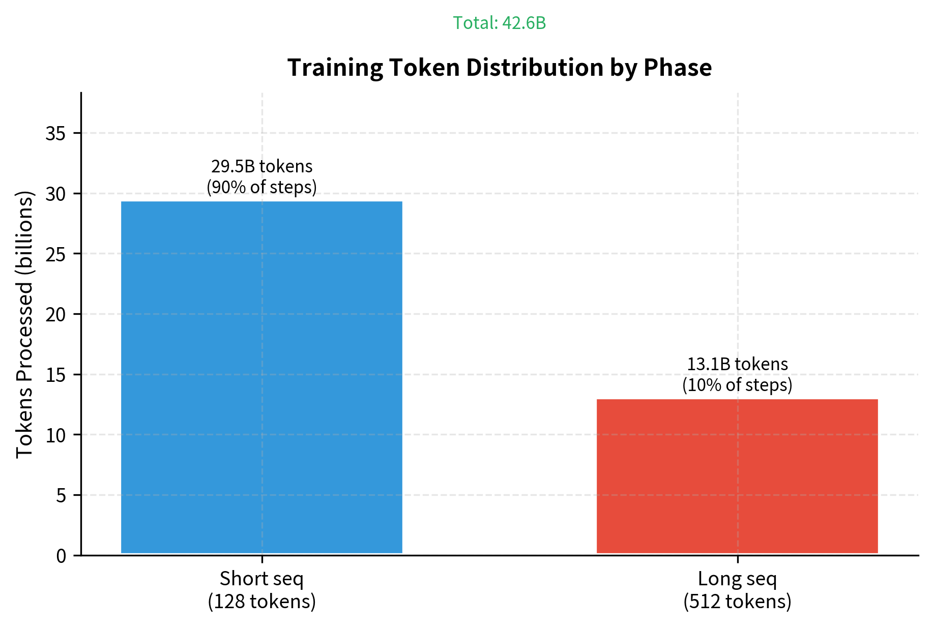
BERT-base processes approximately 40 billion tokens during pre-training. This is roughly 12 passes through the 3.3 billion word corpus, allowing the model to see each token multiple times with different masking patterns.
Model Configurations
BERT comes in two sizes:
| Parameter | BERT-base | BERT-large |
|---|---|---|
| Layers | 12 | 24 |
| Hidden size | 768 | 1024 |
| Attention heads | 12 | 16 |
| Feed-forward size | 3072 | 4096 |
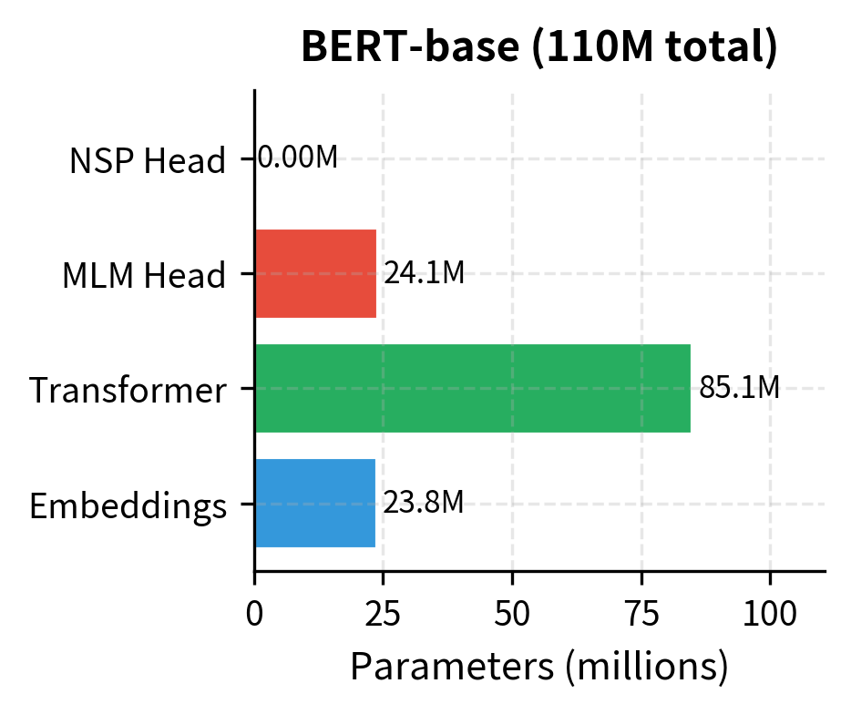
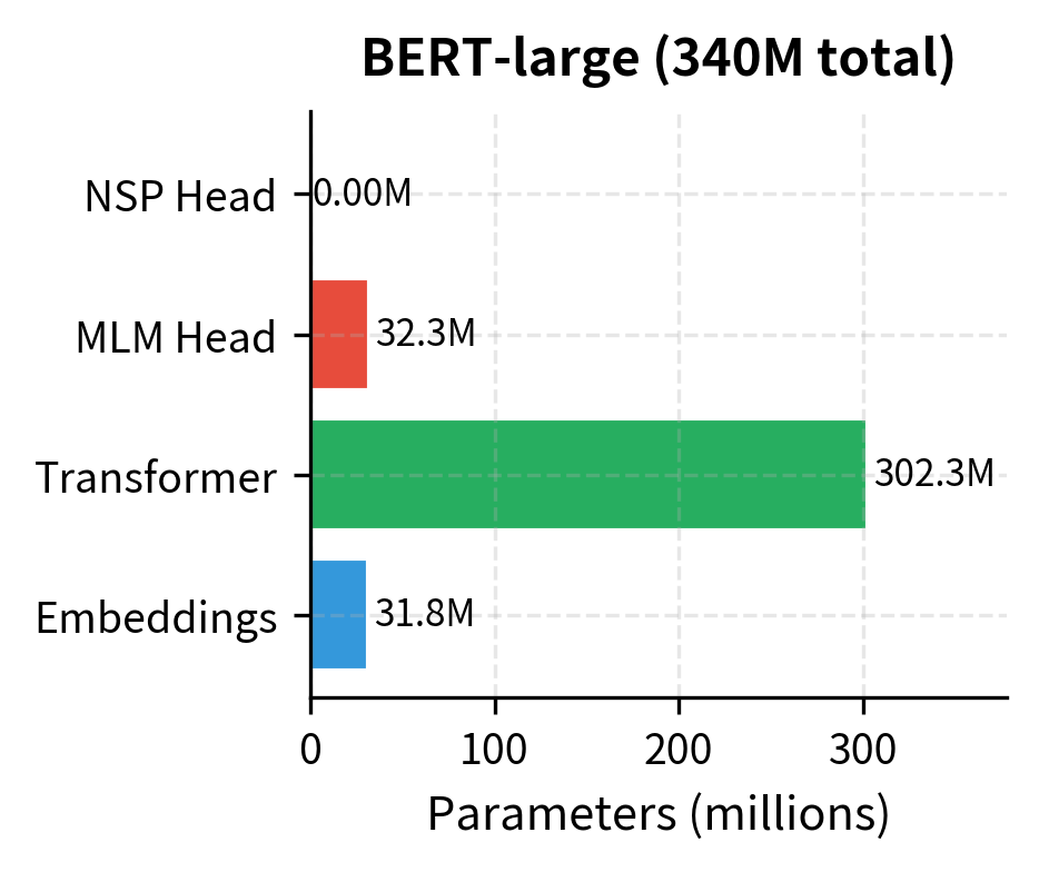
| Parameters | 110M | 340M |
| Pre-training time | ~4 days | ~12 days |
The larger model achieves better performance but requires 3× more compute. Most practitioners use BERT-base because it offers a good balance of quality and efficiency.
The embeddings account for a significant fraction of parameters due to the large vocabulary. The transformer layers dominate in the larger model. The prediction heads are relatively small.
Pre-training Duration and Convergence
How do you know when pre-training is done? BERT trained for 1 million steps, but the loss curve provides more insight than a fixed number.
Loss Curves
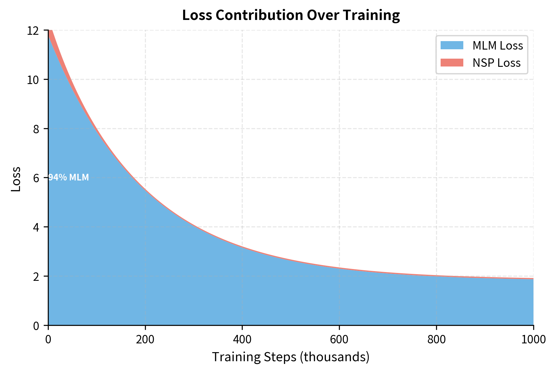
Both MLM and NSP losses decrease rapidly in early training, then gradually level off. The MLM loss typically drops from around 10 (random baseline) to 1.5-2.0. The NSP loss drops from 0.69 (random) to below 0.1.
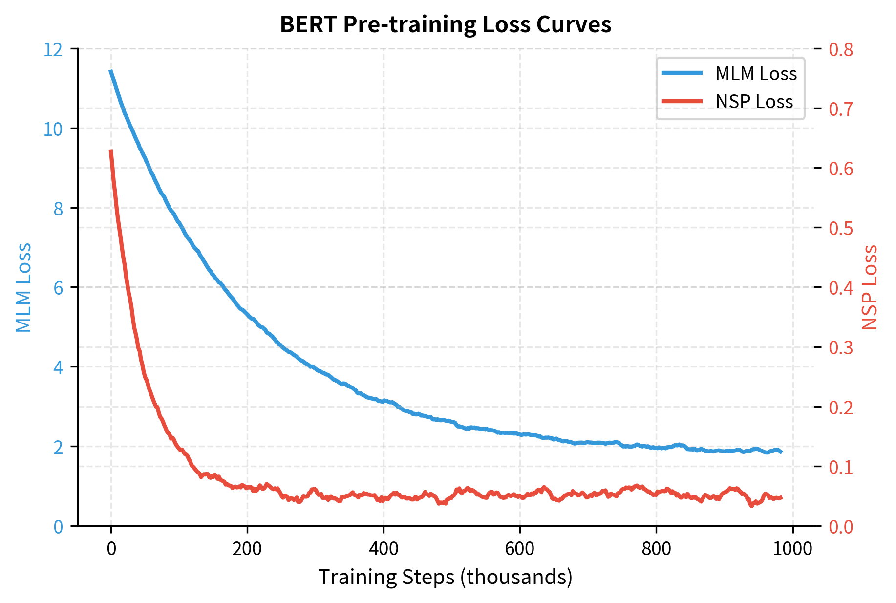
The curves show that NSP converges much faster than MLM. After about 100K steps, the NSP loss is near its final value. MLM continues improving throughout training, though with diminishing returns after 500K steps.
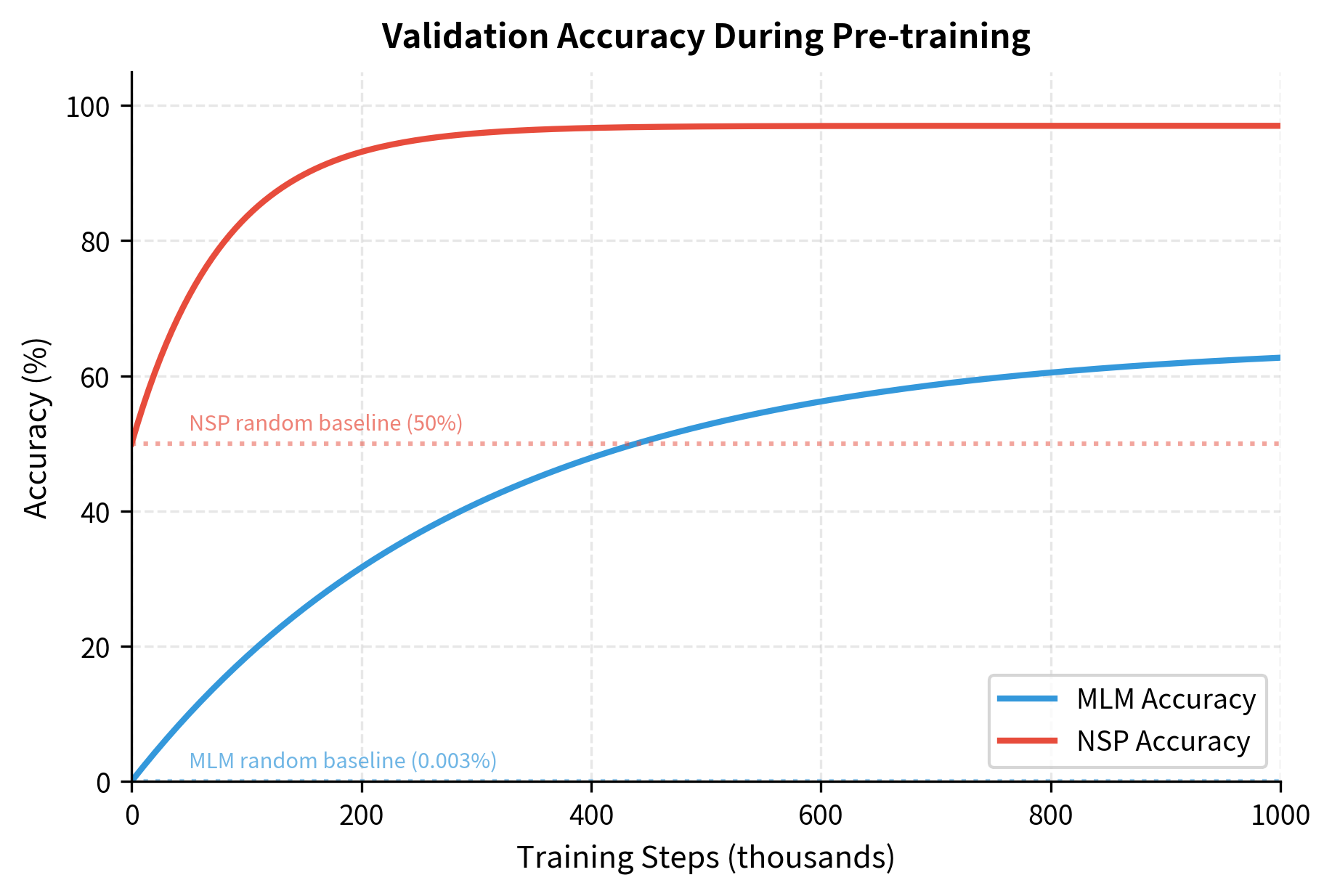
Validation Metrics
During pre-training, the primary metrics are MLM accuracy (fraction of masked tokens correctly predicted) and NSP accuracy. These provide intuition about how well the model is learning.
Typical final values for BERT-base:
- MLM accuracy: 60-65%
- NSP accuracy: 97-98%
The high NSP accuracy reflects that the task is relatively easy. The MLM accuracy of 60% might seem low, but remember the model is predicting from a 30,000-token vocabulary with only surrounding context. Many masked positions have multiple plausible answers.
When to Stop
Pre-training should stop when:
- Loss plateaus: The MLM loss has stopped decreasing for many steps
- Downstream performance peaks: Validation on downstream tasks shows no improvement
- Compute budget exhausted: The allocated resources are fully used
In practice, most BERT variants train for a fixed number of steps (1M for original BERT, 100K for RoBERTa's larger batches) determined empirically. Longer training generally helps until the model begins overfitting to the pre-training corpus.
Putting It All Together
Let's implement a simplified but complete pre-training loop that demonstrates all the components:
This simplified implementation captures the essential pre-training workflow. A production system would add:
- Whole word masking instead of token-level masking
- Dynamic masking (fresh masks each epoch)
- Distributed training across multiple GPUs/TPUs
- Gradient accumulation for larger effective batch sizes
- Mixed precision training for memory efficiency
- Checkpointing and resumption
Limitations and Practical Considerations
BERT's pre-training approach works well, but it comes with constraints that affect how the model can be used.
The compute requirements are substantial. Pre-training BERT-base on 4 TPU v3 chips takes approximately 4 days. BERT-large requires roughly 12 days. For organizations without access to TPU pods or large GPU clusters, pre-training from scratch is impractical. This is why most practitioners start from publicly available checkpoints and fine-tune rather than pre-training. The environmental cost is also non-trivial: training BERT-large once produces CO₂ emissions comparable to a trans-American flight.
The fixed vocabulary constrains domain adaptation. BERT's WordPiece vocabulary was trained on BooksCorpus and Wikipedia. For specialized domains like medicine or law, many terms tokenize into character-level fragments, losing semantic coherence. Continued pre-training on domain-specific text helps, but the vocabulary remains suboptimal. Some projects address this by training entirely new models with domain-specific vocabularies.
NSP's value remains debated. RoBERTa demonstrated that removing NSP entirely and using longer contiguous sequences improved downstream performance. This suggests the original NSP task may have been too easy, providing weak supervision. However, some tasks like question answering that require cross-sentence reasoning may still benefit from sentence-level objectives. The ALBERT paper's Sentence Order Prediction offers a middle ground.
Static masking limits training efficiency. Each training example shows the model the same masked positions across all epochs. Dynamic masking, where positions are re-sampled each epoch, provides more varied training signal. RoBERTa adopted dynamic masking as a default, showing modest improvements.
Key Parameters
The most important parameters when configuring BERT pre-training:
-
mask_prob (default: 0.15): Fraction of tokens selected for masking per sequence. The 15% rate balances learning signal against context preservation. Higher rates (up to 40%) have been explored with mixed results.
-
learning_rate (default: 1e-4): Peak learning rate after warmup. Lower rates (5e-5) may be needed for larger models or smaller batch sizes to prevent instability.
-
warmup_steps (default: 10,000): Number of steps to linearly increase learning rate from 0 to peak. Prevents large gradient updates early in training when loss landscape is rough.
-
batch_size (default: 256): Number of sequences per training batch. Larger batches (up to 8192 with gradient accumulation) improve training efficiency but require more memory.
-
max_seq_length (default: 512): Maximum sequence length the model can process. BERT uses 128 for 90% of training, then 512 for the final 10% to save compute.
-
num_train_steps (default: 1,000,000): Total training steps. More steps generally improve performance until overfitting begins.
-
weight_decay (default: 0.01): L2 regularization coefficient applied to all parameters except biases and LayerNorm. Helps prevent overfitting.
-
positive_ratio (default: 0.5): Fraction of sentence pairs that are actual consecutive sentences versus random pairs for NSP. Balanced 50/50 is standard.
Summary
BERT's pre-training combines two complementary objectives to learn rich language representations:
- Training data from BooksCorpus and Wikipedia provides diverse, high-quality text totaling 3.3 billion words
- Masked Language Modeling forces bidirectional context understanding by predicting randomly masked tokens (15% mask rate, 80-10-10 corruption strategy)
- Next Sentence Prediction adds document-level signal by classifying whether sentence pairs are consecutive (though its value is debated)
- Hyperparameters include AdamW optimizer with linear warmup and decay, 256 batch size, and two-phase sequence length (128 then 512)
- Training duration spans 1 million steps over approximately 4 days for BERT-base, processing roughly 40 billion tokens
- The combined loss equally weights MLM and NSP, allowing both objectives to shape the shared representations
The next chapter explores fine-tuning: how to adapt these pre-trained representations to specific downstream tasks.
Quiz
Ready to test your understanding? Take this quick quiz to reinforce what you've learned about BERT pre-training.

Comments