Linear Attention: Breaking the Quadratic Bottleneck with Kernel Feature Maps

Standard self-attention computes a weighted sum of value vectors, where the weights come from a softmax over query-key similarities. This produces an $n \times n$ attention matrix that must be explicitly computed and stored, leading to the quadratic bottleneck that limits transformers to modest sequence lengths. Linear attention takes a radically different approach: by replacing the softmax with a decomposable kernel function, it enables a clever reordering of matrix operations that eliminates the quadratic term entirely.

The key insight is mathematical: if we can factor the attention weights into a product of separate functions applied to queries and keys, we can change the order of operations from $(QK^T)V$ to $Q(K^TV)$. The first form requires computing the full $n \times n$ attention matrix. The second form computes $K^TV$ first, which has shape $d \times d$ (model dimension squared), independent of sequence length. This simple reordering transforms $O(n^2d)$ complexity into $O(nd^2)$, making attention linear in sequence length.

In this chapter, we explore how linear attention achieves this transformation, examine the kernel feature maps that make it possible, implement the mechanism from scratch, and analyze both its theoretical elegance and practical limitations. We also survey variants like Performer that address some of softmax attention's properties that linear attention initially sacrifices.

To understand linear attention, we need to examine why standard softmax attention requires the $n \times n$ matrix in the first place. The culprit is the softmax normalization, which creates dependencies between all positions.

Standard attention computes:

where:

• $Q \in \mathbb{R}^{n \times d_k}$: the query matrix containing one row per token
• $K \in \mathbb{R}^{n \times d_k}$: the key matrix containing one row per token
• $V \in \mathbb{R}^{n \times d_v}$: the value matrix containing the information to aggregate
• $d_k$: the dimension of query and key vectors
• $n$: the sequence length (number of tokens)
• The softmax is applied row-wise, normalizing each query's attention distribution

For each query position $i$, the attention output is:

where:

• $q_i \in \mathbb{R}^{d_k}$: the query vector at position $i$
• $k_j \in \mathbb{R}^{d_k}$: the key vector at position $j$
• $v_j \in \mathbb{R}^{d_v}$: the value vector at position $j$
• $q_i^T k_j$: the dot product measuring similarity between query $i$ and key $j$
• $\exp(\cdot)$: the exponential function ensuring positive weights
• The denominator sums over all $n$ positions, creating the normalization constant

The denominator is the normalization term: to compute the attention weight for any single key position $j$, we need to know the scores for all positions, because the softmax divides by their sum. This creates a global dependency that forces us to compute all $n^2$ query-key products before we can produce any output.

Linear attention's solution is to replace the exponential-and-normalize pattern with a kernel function that decomposes into separate feature maps for queries and keys. Instead of:

We use:

where:

• $\phi: \mathbb{R}^{d_k} \to \mathbb{R}^{D}$: a feature map that transforms vectors from the original $d_k$-dimensional space to a $D$-dimensional feature space
• $\phi(q_i) \in \mathbb{R}^D$: the transformed query vector
• $\phi(k_j) \in \mathbb{R}^D$: the transformed key vector
• $D$: the dimension of the feature space (often equal to $d_k$ for simple maps, or larger for random feature methods)

The key property is that the similarity decomposes into an inner product of transformed vectors, allowing us to reorder operations using matrix associativity.

With this formulation, the attention output becomes:

Since $\phi(q_i)$ does not depend on $j$, we can factor it out of the sum:

This factorization is the key to linear attention. The numerator contains $\phi(q_i)^T$ multiplied by a sum that doesn't depend on $i$. The denominator has the same structure. Both sums can be computed once and reused for every query position.

Let's define:

• $S = \sum_{j=1}^{n} \phi(k_j) v_j^T$: a matrix of shape $(D \times d_v)$
• $Z = \sum_{j=1}^{n} \phi(k_j)$: a vector of shape $(D,)$

Then the output for each position simplifies to:

where:

• $\phi(q_i)^T S$: a matrix-vector product of shape $(1 \times D) \cdot (D \times d_v) = (1 \times d_v)$, giving the unnormalized output
• $\phi(q_i)^T Z$: a dot product of shape $(1 \times D) \cdot (D \times 1) = 1$, giving the normalization scalar

Computing $S$ requires $O(nd \cdot D)$ operations (summing $n$ outer products of dimension $D \times d_v$). Computing each output requires $O(D \cdot d_v)$ operations. With $n$ outputs, the total complexity is $O(nd^2)$ assuming $D$ is proportional to $d$.

Having established the mathematical foundation, we can now synthesize everything into the complete linear attention formula. The journey from standard attention to linear attention follows a clear logical path: we identified the softmax as the source of the quadratic bottleneck, replaced it with a decomposable kernel function, and discovered that the resulting expression can be rearranged to avoid computing the full attention matrix. Now let's see how these insights combine into a practical algorithm.

We derived earlier that each position's output can be written as:

To express this for all positions simultaneously, we stack the feature-mapped queries into a matrix and apply the same operations in parallel. For a sequence of $n$ tokens with queries $Q$, keys $K$, and values $V$, the complete formula is:

Let's unpack each component to understand how the pieces fit together:

• $\phi(Q) \in \mathbb{R}^{n \times D}$: The feature map $\phi$ applied row-wise to the query matrix. Each of the $n$ query vectors is transformed from $d_k$ dimensions to $D$ dimensions.

• $\phi(K) \in \mathbb{R}^{n \times D}$: Similarly, the feature map applied to each key vector. After transformation, we transpose this to get $\phi(K)^T \in \mathbb{R}^{D \times n}$.

• $\phi(K)^T V$: This is the key-value aggregate $S$ from our derivation. The matrix product has shape $(D \times n) \cdot (n \times d_v) = (D \times d_v)$. Notice that $n$ disappears from the result shape, and this is precisely why linear attention avoids the quadratic bottleneck.

• $\phi(Q)(\phi(K)^T V)$: Multiplying the queries by the aggregate produces the numerator. Shape: $(n \times D) \cdot (D \times d_v) = (n \times d_v)$.

• $\phi(K)^T \mathbf{1}$: Summing the transformed keys (equivalent to $Z$ in our derivation). The vector of ones $\mathbf{1} \in \mathbb{R}^n$ sums across all $n$ key positions, producing a $D$-dimensional vector.

• The division is performed element-wise per row, normalizing each output position by its corresponding scalar denominator.

The formula highlights the critical insight: the order in which we perform matrix multiplications determines the complexity. Consider the numerator $\phi(Q)(\phi(K)^T V)$:

1. If we compute $\phi(Q)\phi(K)^T$ first (as in standard attention), we get an $n \times n$ matrix. Multiplying by $V$ then costs $O(n^2 d_v)$.

2. If we compute $\phi(K)^T V$ first (the linear attention approach), we get a $D \times d_v$ matrix. Multiplying $\phi(Q)$ by this costs only $O(n D d_v)$.

The second approach avoids ever creating the $n \times n$ matrix. This is matrix associativity in action: $(AB)C = A(BC)$, but the intermediate sizes differ dramatically.

When the feature dimension $D$ is proportional to the model dimension $d$ (and $d \ll n$ for long sequences), linear attention provides substantial savings. For a 10,000-token sequence with $d = 64$, standard attention requires a 100-million-element intermediate matrix, while linear attention needs only 4,096 elements.

Let's implement linear attention step by step, mapping each line of code to the mathematical operations we've discussed.

The implementation follows our derivation exactly:

1. Apply the feature map: Transform $Q$ and $K$ to get $\phi(Q)$ and $\phi(K)$. We use ELU+1 as a default because it ensures all features are positive, which is necessary for the normalization to produce valid weights.

2. Compute the key-value aggregate: K_prime.T @ V computes $\phi(K)^T V$, the $D \times d_v$ matrix that summarizes how each feature dimension relates to the values. This is computed once and reused for all queries.

3. Compute the normalization aggregate: K_prime.sum(axis=0) computes $\sum_j \phi(k_j)$, equivalent to $\phi(K)^T \mathbf{1}$. This is the denominator's aggregate.

4. Query the aggregates: Each query retrieves its output by multiplying against the precomputed aggregates. The numerator Q_prime @ KV and denominator Q_prime @ K_sum are both $O(nDd)$ operations.

5. Normalize: Element-wise division produces the final attention output.

Let's run this implementation and verify that it produces the expected shapes and efficiency characteristics.

The output confirms the efficiency gain: instead of a 128×128 attention matrix (16,384 elements), linear attention uses a 64×64 key-value aggregate (4,096 elements). This 4x reduction might seem modest, but remember that the ratio scales as $(n/d)^2$. At 1,024 tokens with $d = 64$, the reduction is 256x. At 8,192 tokens, it's over 16,000x. The quadratic-to-linear improvement becomes increasingly dramatic as sequences grow longer.

The choice of feature map $\phi$ determines the properties of linear attention. Different feature maps approximate different similarity functions, each with trade-offs between computational efficiency and how well they mimic softmax behavior.

The connection between feature maps and attention kernels comes from the theory of reproducing kernel Hilbert spaces (RKHS). A kernel function $\kappa(x, y)$ measures similarity between two vectors, and Mercer's theorem tells us that any positive semi-definite kernel can be written as:

where:

• $\kappa: \mathbb{R}^d \times \mathbb{R}^d \to \mathbb{R}$: a kernel function that takes two vectors and returns a scalar similarity score
• $x, y \in \mathbb{R}^d$: input vectors to compare
• $\phi: \mathbb{R}^d \to \mathbb{R}^D$: a feature map that lifts inputs to a (possibly infinite-dimensional) feature space
• $\langle \cdot, \cdot \rangle$: the inner product in the feature space

This result, known as Mercer's theorem, tells us that for any valid kernel function, there exists a corresponding feature map. Choosing a feature map implicitly defines a similarity kernel, and vice versa.

Standard softmax attention uses an exponential kernel (ignoring the scaling factor):

where $q^T k$ is the dot product between query and key vectors. The exponential function ensures the similarity is always positive and amplifies differences between scores.

To approximate this with linear attention, we need a feature map $\phi$ such that:

Finding such a feature map is the central challenge of linear attention design. The closer the approximation, the more closely linear attention mimics softmax behavior.

Several feature maps have been proposed, each with different properties:

1. ELU + 1 (Efficient Linear Units)

This simple feature map ensures all features are positive (required for the normalization to work properly). It doesn't approximate the exponential kernel well but is computationally cheap.

2. ReLU

Even simpler than ELU, but can produce zero features, potentially causing numerical issues in the denominator.

3. Random Fourier Features (Performer)

where:

• $x \in \mathbb{R}^{d_k}$: the input vector (query or key)
• $m$: the number of random frequency vectors
• $\omega_i \in \mathbb{R}^{d_k}$: random frequency vectors sampled from a standard normal distribution $\mathcal{N}(0, I)$
• $\omega_i^T x$: the projection of input onto the $i$-th random direction
• $\frac{1}{\sqrt{m}}$: normalization factor to control the variance of the approximation

The output has dimension $2m$ (sine and cosine for each frequency). This provides an unbiased approximation to the Gaussian kernel. With additional scaling, it can approximate the softmax kernel.

4. Positive Random Features (FAVOR+)

To ensure non-negativity while approximating the exponential kernel, Performer uses:

where:

• $x \in \mathbb{R}^{d_k}$: the input vector
• $\|x\|^2 = \sum_{i=1}^{d_k} x_i^2$: the squared Euclidean norm of the input
• $\exp(-\|x\|^2/2)$: a normalization factor that depends on the input magnitude
• $\omega_i \sim \mathcal{N}(0, I)$: random projection vectors sampled from a standard normal distribution
• $\exp(\omega_i^T x)$: ensures all features are strictly positive
• $m$: the number of random features

This construction gives $\mathbb{E}[\phi(q)^T \phi(k)] = \exp(q^T k)$, an unbiased estimator of the softmax kernel. The key insight is that by using exponentials instead of sines and cosines, all features remain positive, which is necessary for the normalization in attention to work correctly.

The ELU and ReLU maps preserve the input dimension, making them computationally efficient. Random feature maps expand to a higher dimension, trading compute for better approximation of the softmax kernel.

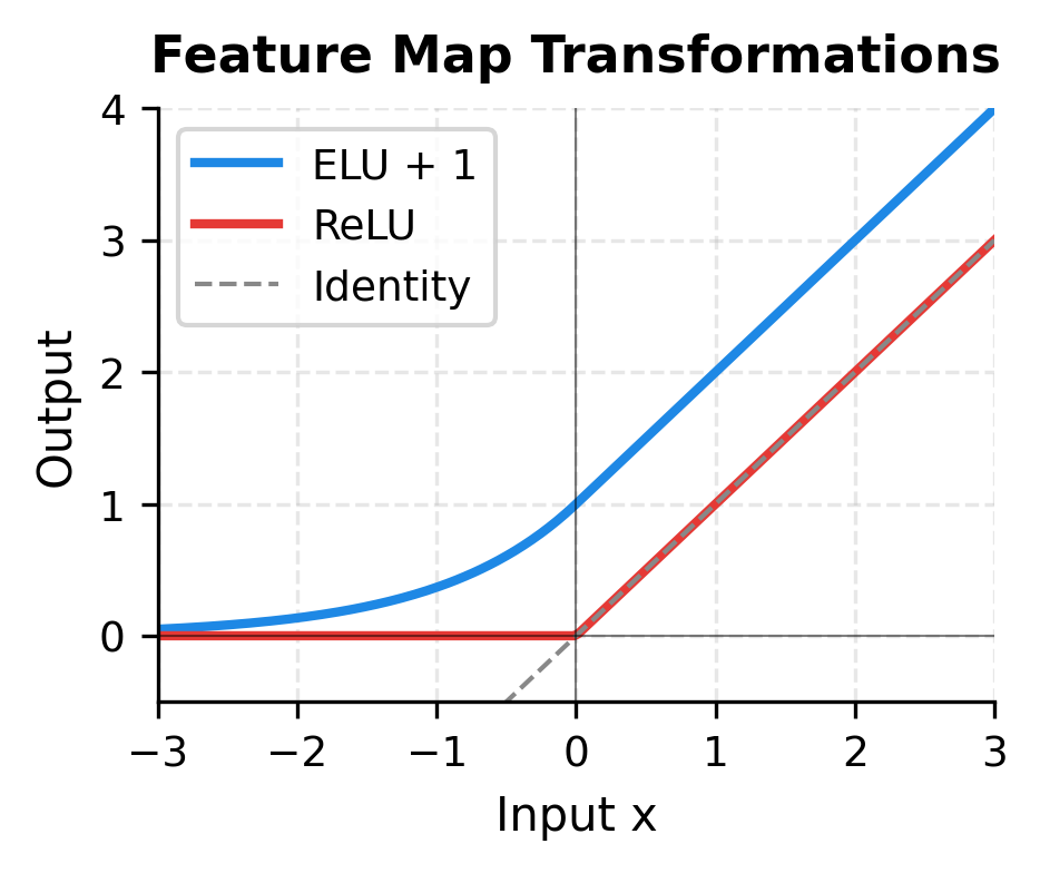
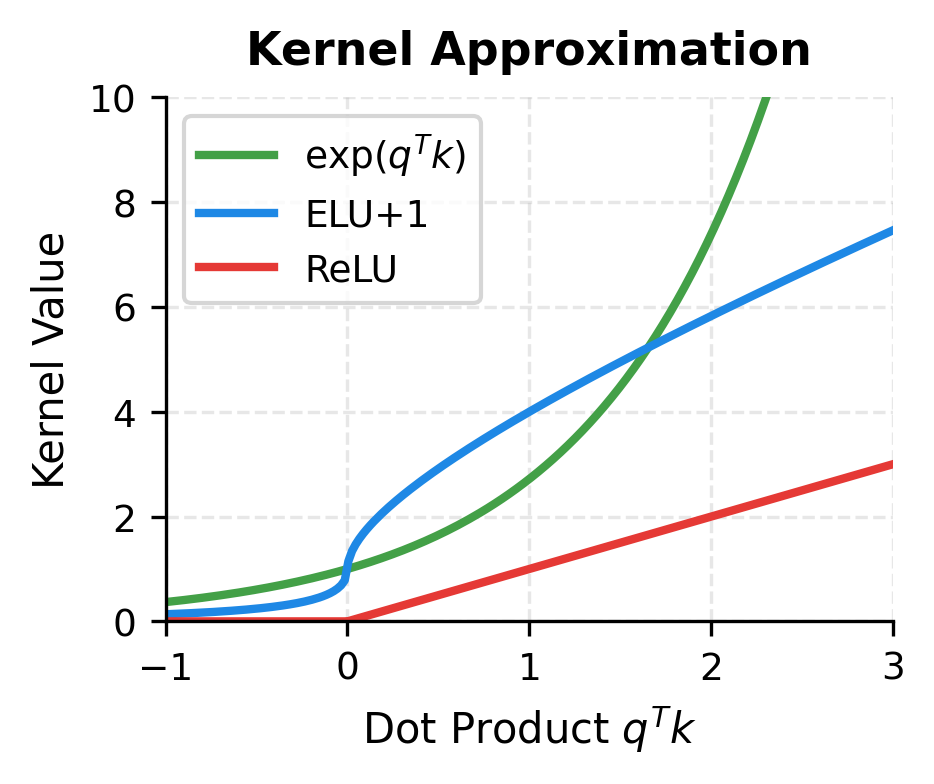
The visualizations reveal key properties of the feature maps. ELU+1 produces strictly positive outputs for all inputs, which is essential for attention normalization. ReLU is simpler but zeros out negative inputs, losing information and potentially causing numerical issues. Neither simple feature map accurately approximates the exponential kernel, especially for larger dot products, which explains why they produce different attention patterns than softmax.

Let's implement both attention mechanisms and compare their outputs to understand what linear attention preserves and what it changes.

The cosine similarity shows that linear attention with a simple ELU feature map produces outputs that point in a similar direction to standard attention but aren't identical. The MSE quantifies the actual difference in output values.

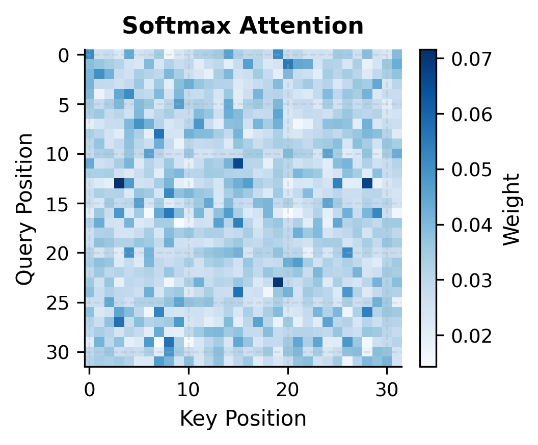
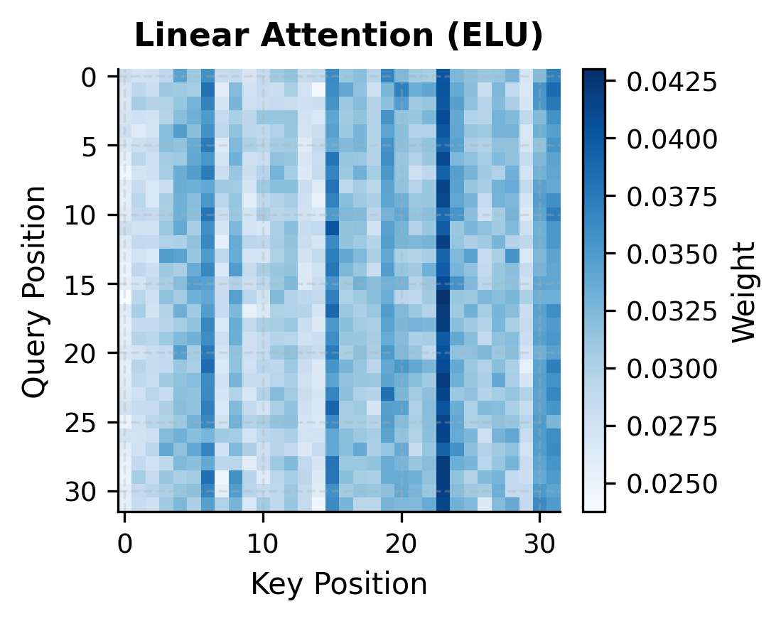
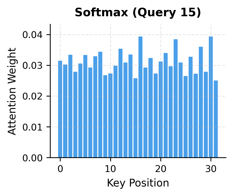
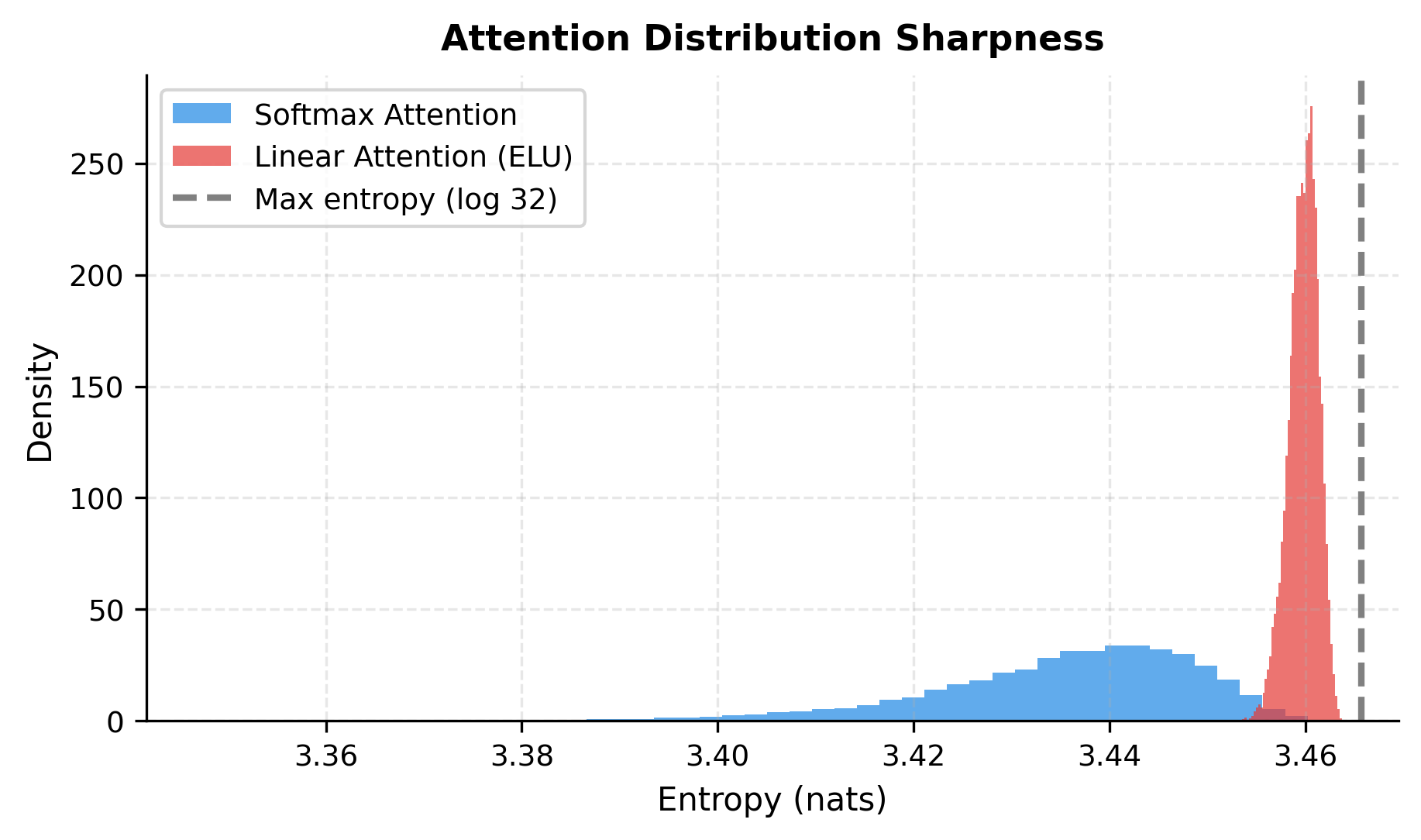
The visualizations reveal a fundamental difference in attention behavior. Softmax attention concentrates weight on a few key positions, creating the "sharp" attention patterns that transformers are known for. Linear attention with simple feature maps spreads weight more uniformly, producing softer patterns that may miss fine-grained dependencies.

Let's rigorously compare the computational requirements of standard and linear attention across different sequence lengths.

The speedup grows linearly with sequence length. At 128 tokens, linear attention is only marginally faster. At 16,384 tokens, it's over 100x faster. This is the power of eliminating the quadratic term: the longer the sequence, the greater the benefit.

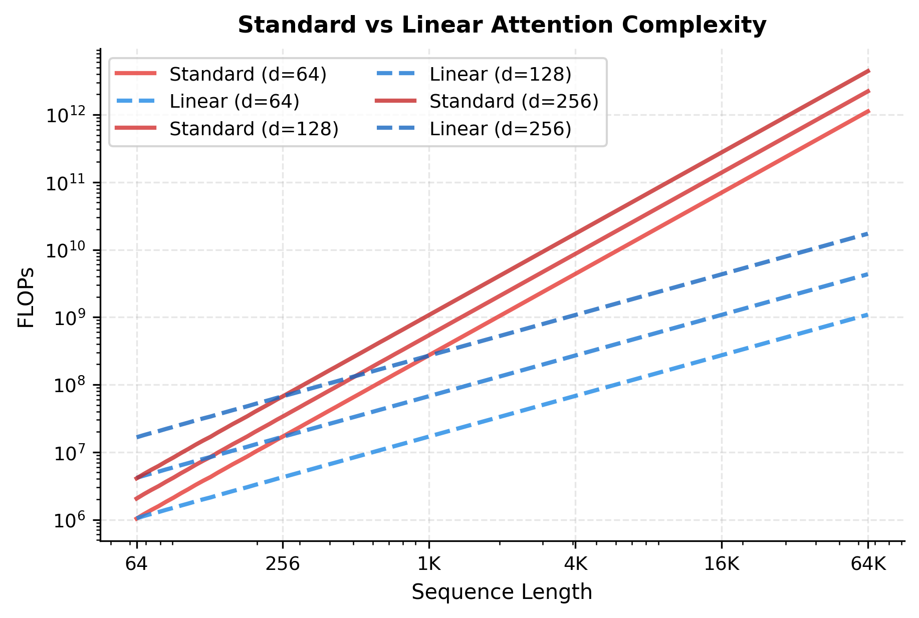
The log-scale plot reveals the essential difference: standard attention curves have slope 2 (quadratic), while linear attention curves have slope 1 (linear). All curves for the same algorithm are parallel, shifted only by the constant factor from the model dimension.

Beyond compute savings, linear attention also dramatically reduces memory requirements. Standard attention must store the full $n \times n$ attention matrix during the forward pass (for use in backpropagation). Linear attention only stores the $d \times d$ key-value aggregate.

At 16,384 tokens, standard attention requires over 1 GB just for the attention matrix, while linear attention uses only about 16 KB. This memory efficiency is what enables linear attention to scale to extremely long sequences that would be impossible with standard attention.

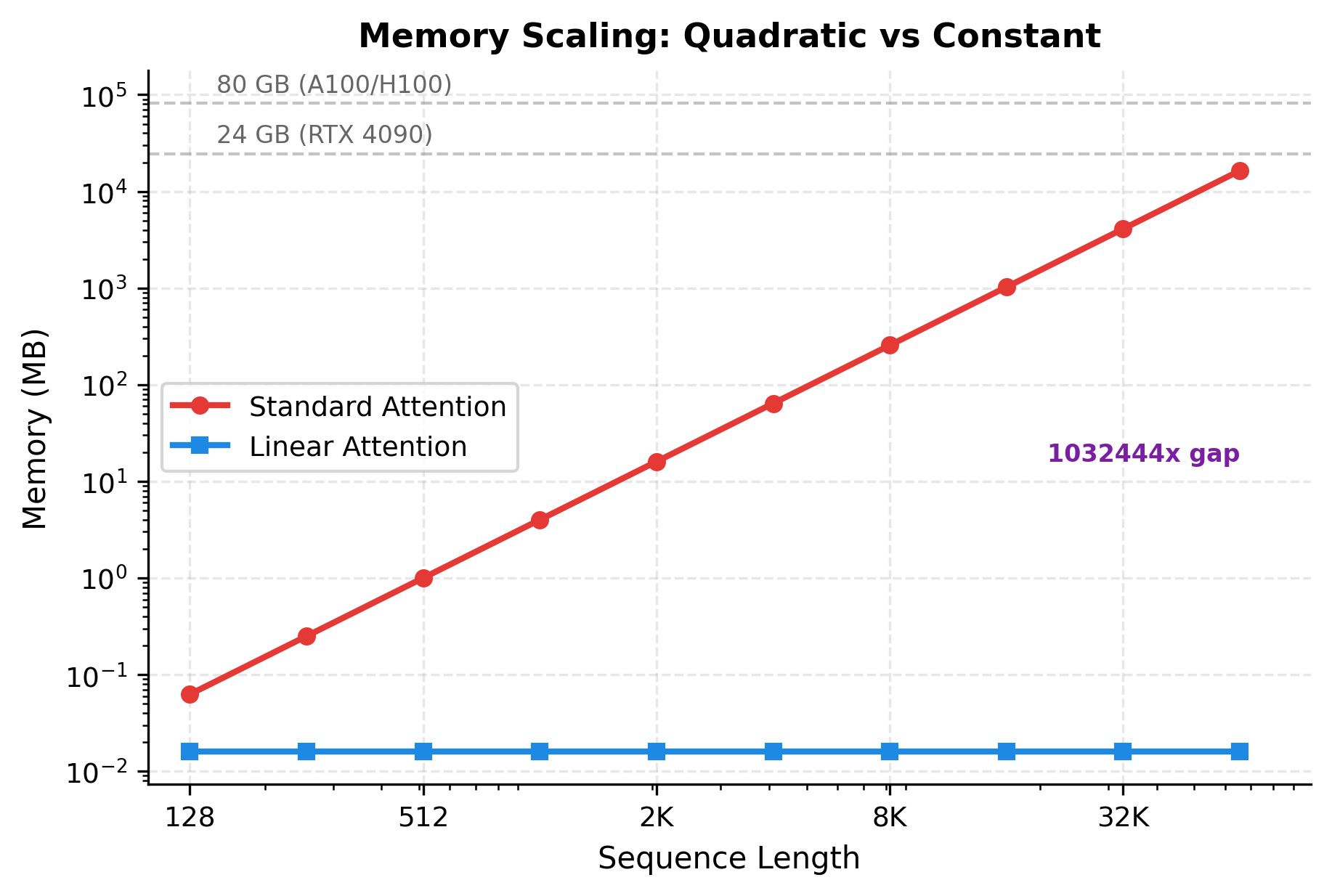
The log-log visualization makes the scaling difference stark. Standard attention memory grows as a straight line with slope 2 (quadratic), while linear attention remains essentially flat at around 16 KB regardless of sequence length. At 65,536 tokens, standard attention would require over 16 GB just for the attention matrix, exceeding even high-end GPU memory, while linear attention uses the same 16 KB it needed at 128 tokens.

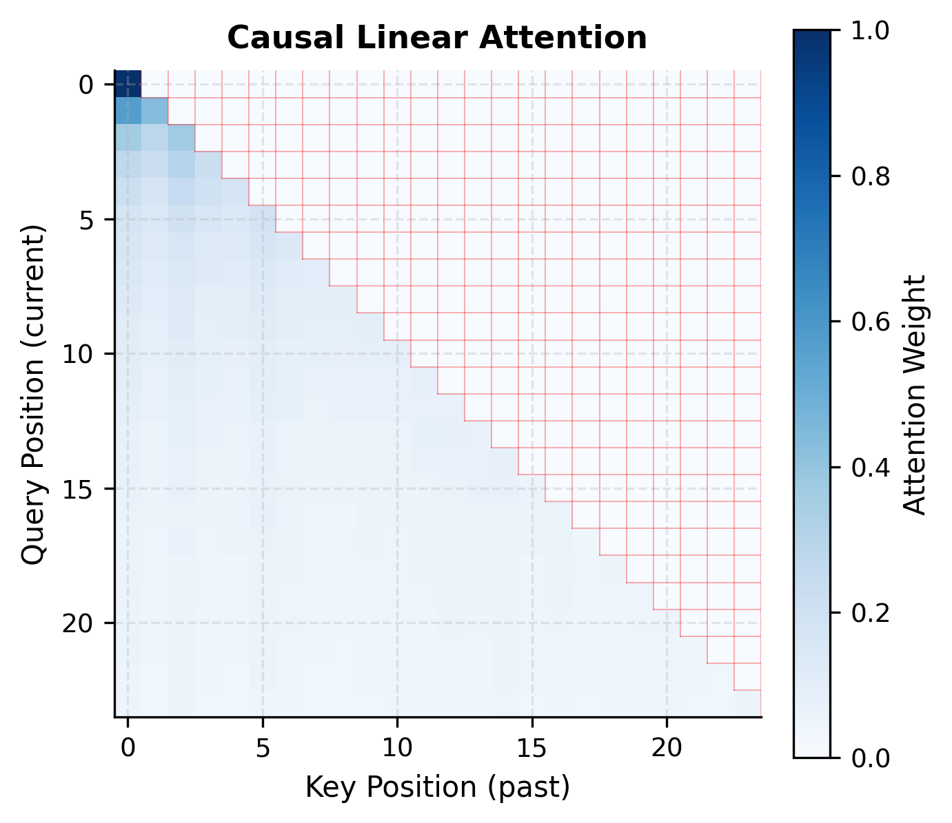
For autoregressive language models, we need causal attention: each position can only attend to previous positions. Standard causal attention applies a triangular mask before softmax. Linear attention requires a different approach.

The key insight is that the key-value aggregate can be computed incrementally. Instead of summing over all positions, we maintain a running sum up to the current position:

where:

• $S_i \in \mathbb{R}^{D \times d_v}$: the cumulative key-value aggregate up to position $i$, computed by summing outer products $\phi(k_j) v_j^T$ for all positions $j \leq i$
• $Z_i \in \mathbb{R}^{D}$: the cumulative key sum up to position $i$, used for normalization
• $\phi(q_i)^T S_i$: retrieves a weighted combination of values based on the query at position $i$
• $\phi(q_i)^T Z_i$: computes the normalization factor

This formulation naturally respects causality: position $i$ only accesses information from positions $1$ through $i$. The running sum structure enables efficient incremental computation during inference.

The causal formulation is particularly elegant because the running sum structure means that during inference, we can process one token at a time with $O(1)$ memory overhead per step (just updating the $d \times d$ aggregate). This makes linear attention ideal for autoregressive generation.

The simple feature maps we've examined (ELU, ReLU) don't approximate softmax attention well. Performer, introduced by Choromanski et al. in 2020, addresses this with a clever approach called FAVOR+ (Fast Attention Via positive Orthogonal Random features).

The goal is to find a feature map $\phi$ such that:

where:

• $\mathbb{E}[\cdot]$: the expectation operator, averaging over the random projection vectors
• $\phi(q)^T \phi(k)$: the inner product of feature-mapped query and key
• $\exp(q^T k)$: the true softmax kernel (without the scaling factor)

When this equality holds in expectation, we say the approximation is unbiased: on average, linear attention produces the same result as softmax attention. Performer achieves this by using positive random features:

where $\omega_i \sim \mathcal{N}(0, I)$ are random projection vectors drawn from a standard normal distribution, and $m$ is the number of random features that controls the trade-off between approximation quality and computational cost.

The results show that Performer's approximation improves with more random features. With 512 features, the cosine similarity approaches 1.0 and MSE drops significantly. This trade-off between approximation quality and feature dimension is central to Performer's design: more features mean better approximation but higher compute cost.

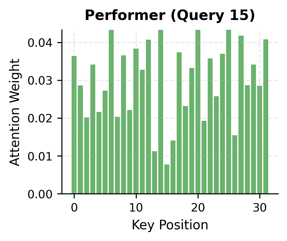
Performer's key innovation is that by using positive features with the right normalization, the approximation is unbiased: the expected value equals true softmax attention. The variance of the approximation decreases as $O(1/m)$, where $m$ is the number of random features. This means doubling the number of features halves the variance, providing a controllable trade-off between computational cost and approximation fidelity.

The linear attention family has grown to include many variants, each addressing different aspects of the softmax-to-kernel trade-off:

• Linear Transformer (Katharopoulos et al., 2020): The foundational work that established the kernel view and demonstrated causal linear attention for autoregressive models.

• Random Feature Attention (RFA): Uses random Fourier features to approximate the Gaussian kernel, providing a middle ground between simple feature maps and Performer's FAVOR+.

• Nyströmformer (Xiong et al., 2021): Uses the Nyström method to approximate the attention matrix with landmark points, achieving $O(nm)$ complexity where $m$ is the number of landmarks.

• FNet (Lee-Thorp et al., 2021): Replaces attention entirely with Fourier transforms, achieving $O(n \log n)$ complexity with no learnable attention parameters.

• RetNet (Sun et al., 2023): Combines linear attention with exponential decay, creating a recurrent formulation that supports both parallel training and efficient incremental inference.

Linear attention with ELU features achieves approximately 64x speedup over standard softmax attention at this sequence length, while Performer with 256 random features achieves around 60x. The simpler variants (Nyströmformer, FNet) offer even greater speedups but with different quality trade-offs.

Linear attention's efficiency comes with trade-offs. Understanding these limitations is essential for choosing when to use linear attention versus other approaches.

Reduced Expressiveness: Softmax attention can create arbitrarily sharp attention patterns, focusing nearly all weight on a single position. The kernel decomposition in linear attention constrains the types of attention patterns that can be expressed. With simple feature maps like ELU, linear attention tends toward smoother, more diffuse patterns that may not capture fine-grained dependencies as precisely. This is particularly problematic for tasks requiring exact matching or retrieval from context.

Approximation Error: Random feature methods like Performer introduce variance in the attention computation. While the expected value matches softmax attention, individual forward passes have stochastic deviations. For tasks with low tolerance for noise (like copying or exact arithmetic), this variance can hurt performance. Increasing the number of random features reduces variance but increases compute cost, partially eroding the efficiency gains.

Challenges with Causal Modeling: While causal linear attention is theoretically elegant, the running sum formulation has practical issues. The cumulative nature means errors can compound over long sequences. Additionally, the lack of true position-wise softmax normalization means that earlier positions in the sequence may receive disproportionate total attention weight, creating position biases that don't exist in standard causal attention.

Training Stability: Some linear attention variants, particularly those with simple feature maps, can exhibit training instabilities. The normalization in linear attention (dividing by the sum of key features) can have high variance when key features are poorly conditioned. This often requires careful initialization and potentially learning rate adjustments.

Despite these limitations, linear attention remains valuable for specific use cases. Long-document understanding, where the quadratic bottleneck is most severe, benefits enormously from linear complexity. Streaming applications that process tokens incrementally can leverage the recurrent formulation. And hybrid architectures that combine sparse attention layers with occasional linear attention layers get the best of both worlds.

When implementing linear attention in practice, several engineering details matter:

Numerical Stability: The division by the sum of key features can be unstable when the denominator is small. Always add a small epsilon (typically 1e-6) to prevent division by zero. For extreme cases, clipping the denominator to a minimum value may be necessary.

Feature Map Selection: For production systems, the choice of feature map significantly impacts both quality and speed. ELU+1 is fast but produces poor approximations. FAVOR+ provides better approximation but requires generating and storing random projection matrices. A common compromise is to use a deterministic feature map based on learned projections.

Chunked Computation: For very long sequences, even linear attention's memory can be substantial. Computing the KV aggregate in chunks and accumulating helps manage memory, especially on GPUs with limited VRAM.

Linear attention transforms the attention mechanism from quadratic to linear complexity by exploiting the associative property of matrix multiplication. Instead of computing the full $n \times n$ attention matrix, it precomputes a $d \times d$ key-value aggregate that can be queried by each position independently.

The key concepts covered in this chapter:

• Kernel decomposition: Replacing softmax with a kernel function $\kappa(q, k) = \phi(q)^T\phi(k)$ enables reordering $(QK^T)V$ to $Q(K^TV)$, eliminating the quadratic dependency on sequence length.

• Feature maps: Different choices of $\phi$ trade off between computational efficiency and how well they approximate softmax attention. Simple maps like ELU are fast but imprecise; random feature methods like FAVOR+ provide unbiased approximation with controllable variance.

• Causal formulation: Linear attention naturally supports autoregressive modeling through a running sum formulation that incrementally accumulates key-value aggregates, enabling $O(1)$ per-token generation.

• Performer and variants: The FAVOR+ approach uses positive random features to provide an unbiased estimator of softmax attention, with approximation quality improving as the number of random features increases.

• Trade-offs: Linear attention sacrifices the ability to express arbitrarily sharp attention patterns, introduces approximation variance with random features, and may exhibit position biases in causal settings. These limitations make it best suited for long-document tasks where the quadratic bottleneck is the primary constraint.

Linear attention represents a fundamental shift in how we think about the attention mechanism: from an $n \times n$ interaction matrix to a fixed-size state that summarizes the key-value relationships. This perspective has influenced subsequent architectures like state space models and linear recurrent units, which further develop the idea of maintaining a compact state that captures sequence information.

For practitioners, linear attention is most valuable when sequence length is the binding constraint. At shorter lengths where $n < d$, the overhead of feature transformation may not be worthwhile. But for tasks involving documents, books, or streaming data where sequences stretch to tens of thousands of tokens, linear attention's $O(nd^2)$ complexity makes previously intractable problems accessible.

When implementing or tuning linear attention, these parameters most directly affect performance and quality:

• feature_map: The function $\phi$ that transforms queries and keys. ELU+1 is fast and simple but produces poor softmax approximation. FAVOR+ with positive random features provides unbiased approximation but requires more computation. The choice depends on whether you prioritize speed or fidelity to softmax behavior.

• num_features (m): For random feature methods like Performer, this controls the trade-off between approximation quality and computational cost. Higher values reduce variance ($O(1/m)$) but increase the feature dimension. Typical values range from 64 to 512, with 256 offering a reasonable balance for most applications.

• eps: A small constant (typically 1e-6) added to the denominator during normalization to prevent division by zero. Critical for numerical stability, especially when feature maps can produce near-zero values.

• min_denom: An optional floor for the denominator (e.g., 1e-4) that clips extreme values. Useful when the sum of key features is poorly conditioned, which can occur with certain feature maps or input distributions.

• chunk_size: For memory-efficient implementations, this controls how many positions are processed together when accumulating the key-value aggregate. Smaller chunks reduce peak memory usage but may incur overhead from loop iterations. Values between 256 and 1024 work well in practice.

• D (feature dimension): The output dimension of the feature map. For simple maps like ELU, this equals the input dimension $d_k$. For random feature methods, it can be larger than $d_k$ to improve approximation quality, with typical ratios of 2x to 4x the original dimension.

Ready to test your understanding? Take this quick quiz to reinforce what you've learned about linear attention and how it achieves linear complexity.