

Learn how memory-augmented transformers extend context beyond attention limits using external key-value stores, retrieval mechanisms, and compression strategies.

This article is part of the free-to-read Language AI Handbook
Choose your expertise level to adjust how many terms are explained. Beginners see more tooltips, experts see fewer to maintain reading flow. Hover over underlined terms for instant definitions.
Memory Augmentation
Standard transformers compress all context into a fixed-size hidden state. When processing a 100K token document, every piece of information must survive through the attention mechanism's weighted averaging. Important details from early in the document compete against recent tokens for the model's limited representational capacity. Memory augmentation offers an alternative: give the model explicit storage where it can write and retrieve information on demand.
The core insight is straightforward. Instead of forcing the model to implicitly remember everything through its weights and hidden states, we provide an external memory bank. The model can write key-value pairs to this memory during processing and query it when generating outputs. This separation of storage from computation enables effectively unlimited context while keeping each attention operation tractable.
The Memory Bottleneck in Transformers
Before diving into memory architectures, let's understand precisely why standard transformers struggle with long sequences. The problem isn't just computational cost. It's fundamental to how attention aggregates information.
In self-attention, each token produces a query that attends over all key-value pairs from previous positions. The attention weights must sum to 1 due to softmax normalization. With a 100K token context, each previous token receives on average only 0.001% of the attention mass. If the model needs to retrieve a specific fact from 50K tokens ago, it must somehow allocate significant attention weight to that precise location while mostly ignoring the 99,999 other positions.
The table reveals the severity of attention dilution. With uniform attention over a 100K context, each position receives only 0.001% of the attention mass. Even with focused attention (where the model concentrates on the top positions), each selected position only receives about 0.32% of the total weight. The longer the context, the harder it becomes to allocate sufficient attention to any single relevant position.
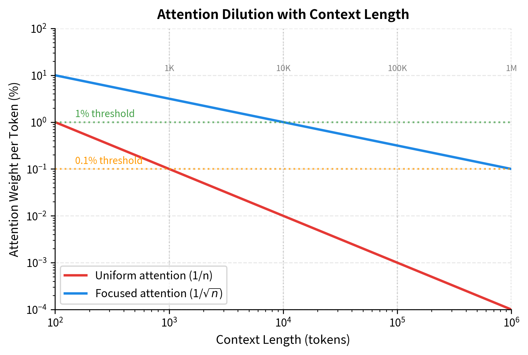
Even with focused attention, retrieving information from a 100K context requires the model to correctly select that position from among approximately 316 candidate slots. This number comes from the square root of the context length: . If the model can only meaningfully attend to the top positions (where is the context length), then it must route attention to the right location among those 316 candidates without knowing in advance where relevant information lies.
The memory bottleneck in transformers refers to the fundamental tension between context length and information retrieval precision. As context grows, attention becomes increasingly diluted, making it harder to retrieve specific information from distant positions. Memory augmentation addresses this by providing explicit storage separate from the attention mechanism.
Memory-augmented architectures sidestep this bottleneck by decoupling storage from the attention computation. The model can write important information to memory during one pass and retrieve it precisely during another, without competing for attention mass against the entire context.
Memory Network Fundamentals
Imagine you're reading a 500-page novel and someone asks you, "What color was the protagonist's childhood home?" You don't re-read the entire book. Instead, your mind somehow retrieves that specific detail from storage. Memory networks attempt to give neural networks this same capability: the ability to write information to an external store during processing and retrieve it on demand.
The Key Insight: Separate Storage from Computation
The fundamental innovation of memory networks is decoupling what the model remembers from how it processes information. In a standard neural network, "memory" exists implicitly in the hidden states, and information must survive through layer after layer of transformation. In a memory network, we provide an explicit storage mechanism that the model can query independently.
This separation immediately suggests two operations:
- Writing: The model encounters important information and stores it
- Reading: The model needs information and retrieves it from storage
But how should storage be organized? And how does the model know where to look when reading?
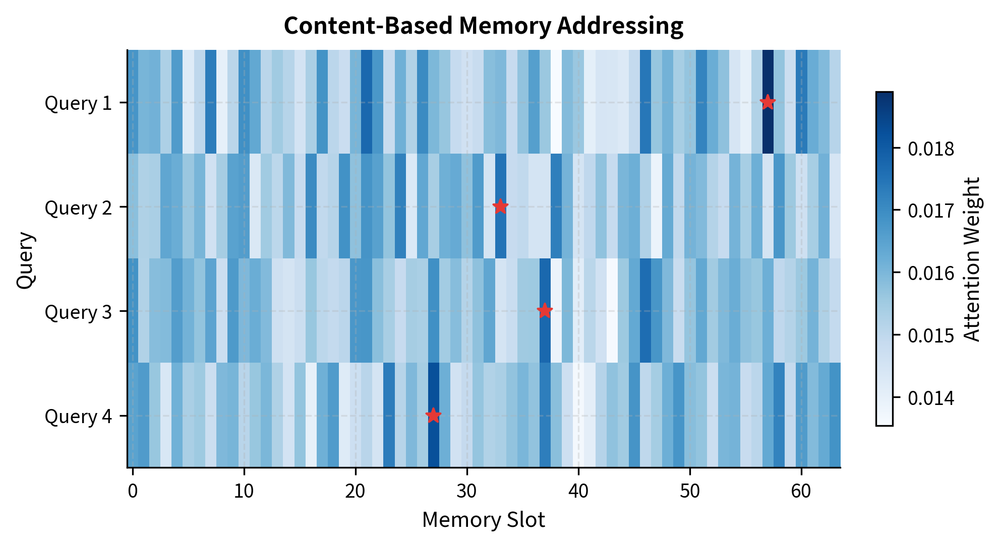
Content-Based Addressing: Finding Information by What It Contains
Consider how you might organize a library. You could assign each book a numbered shelf (positional addressing), or you could organize books by topic and keywords (content-based addressing). A positional system requires remembering exactly where you put each book. A content-based system lets you find books by describing what you're looking for.
Memory networks use content-based addressing. Each memory entry consists of two parts:
- A key : describes what the entry contains (like a book's title and keywords)
- A value : the actual stored content (like the book itself)
When the model wants to retrieve information, it provides a query describing what it's looking for. The memory system compares this query against all stored keys and returns the values whose keys match best.
The Mathematics of Matching: Similarity and Softmax
How do we measure whether a query matches a key? The most natural choice is the dot product. Given a query vector and a key vector , their similarity is:
where:
- is the query vector with dimension
- is the key for memory slot
- is the scalar similarity score
This score tells us how well the query aligns with each key. Larger positive values indicate better matches. But we need to convert these raw scores into a probability distribution, a set of weights that sum to 1, telling us how much to trust each memory entry.
The softmax function accomplishes this. For memory slots with similarity scores :
The exponential ensures all weights are positive (since for all ). The denominator normalizes so that . The weight can be interpreted as "the probability that memory slot contains what we're looking for."
Scaling for Stable Gradients
In practice, we add one refinement. When the dimension is large, dot products can become very large in magnitude. This pushes softmax outputs toward extreme values (nearly 0 or nearly 1), which causes gradient problems during training. The solution is scaled dot-product attention:
Why ? If each component of and has variance 1, then the dot product has variance (since we're summing independent products). Dividing by restores unit variance, keeping the scores in a well-behaved range regardless of dimension.
Retrieving the Answer: Weighted Combination
Once we have attention weights over all memory slots, we retrieve information by taking a weighted sum of the stored values:
where:
- is the retrieved vector (output)
- is the value stored in memory slot
- is the attention weight computed above
This weighted sum is fully differentiable, meaning gradients can flow back through the retrieval operation during training. The model learns which keys to associate with which values by receiving gradient signals about whether the retrieved information helped with the task.
Putting It Together: The Complete Memory Read
The full memory read operation combines all these steps:
where:
- is the matrix of all keys stacked as rows
- is the matrix of all values stacked as rows
- computes all similarity scores in parallel
This is identical to the attention mechanism used in transformers. The difference is conceptual: in standard self-attention, keys and values come from the input sequence; in a memory network, they come from an external storage that persists across inputs.
Implementation: A Basic Memory Network
Let's translate these mathematical concepts into working code. The implementation directly mirrors the formulas above:
The output reveals how attention weights distribute across memory slots. Even with random initialization (where keys and queries have no learned relationship), the softmax produces a sparse pattern. The top 5 slots capture a significant fraction of total attention mass, demonstrating the inherent focusing behavior of the exponential function. After training, these weights would reflect genuine content similarity, with the model having learned to store related information under similar keys.
Memory Retrieval Mechanisms: From Soft to Efficient
The basic memory read operation we just implemented has an elegant mathematical formulation, but it harbors a serious scalability problem. Let's understand this issue deeply before exploring solutions.
The Soft Attention Baseline
Our memory read computes attention over all memory slots:
This soft attention approach has an important advantage: it's fully differentiable. Gradients flow smoothly from the output through the softmax and into the query and key representations. The model can learn what to store and how to query through standard backpropagation.
But soft attention also inherits the same dilution problem we identified earlier for long-context transformers. When is large, each slot's weight becomes vanishingly small. The information we need gets drowned in a weighted average dominated by irrelevant entries.
Temperature: Controlling the Focus-Diffusion Tradeoff
One way to combat dilution is to sharpen the attention distribution. We can introduce a temperature parameter that scales the scores before softmax:
The temperature controls the "peakiness" of the distribution:
-
Low temperature (): Amplifies score differences. Small advantages become large, concentrating attention on the best-matching entries. In the limit , this approaches hard argmax selection.
-
High temperature (): Dampens score differences. The distribution becomes more uniform, spreading attention across many entries.
We can measure this effect through entropy, which quantifies how spread out a distribution is:
Low entropy means attention is concentrated on few slots; high entropy means it's spread across many.
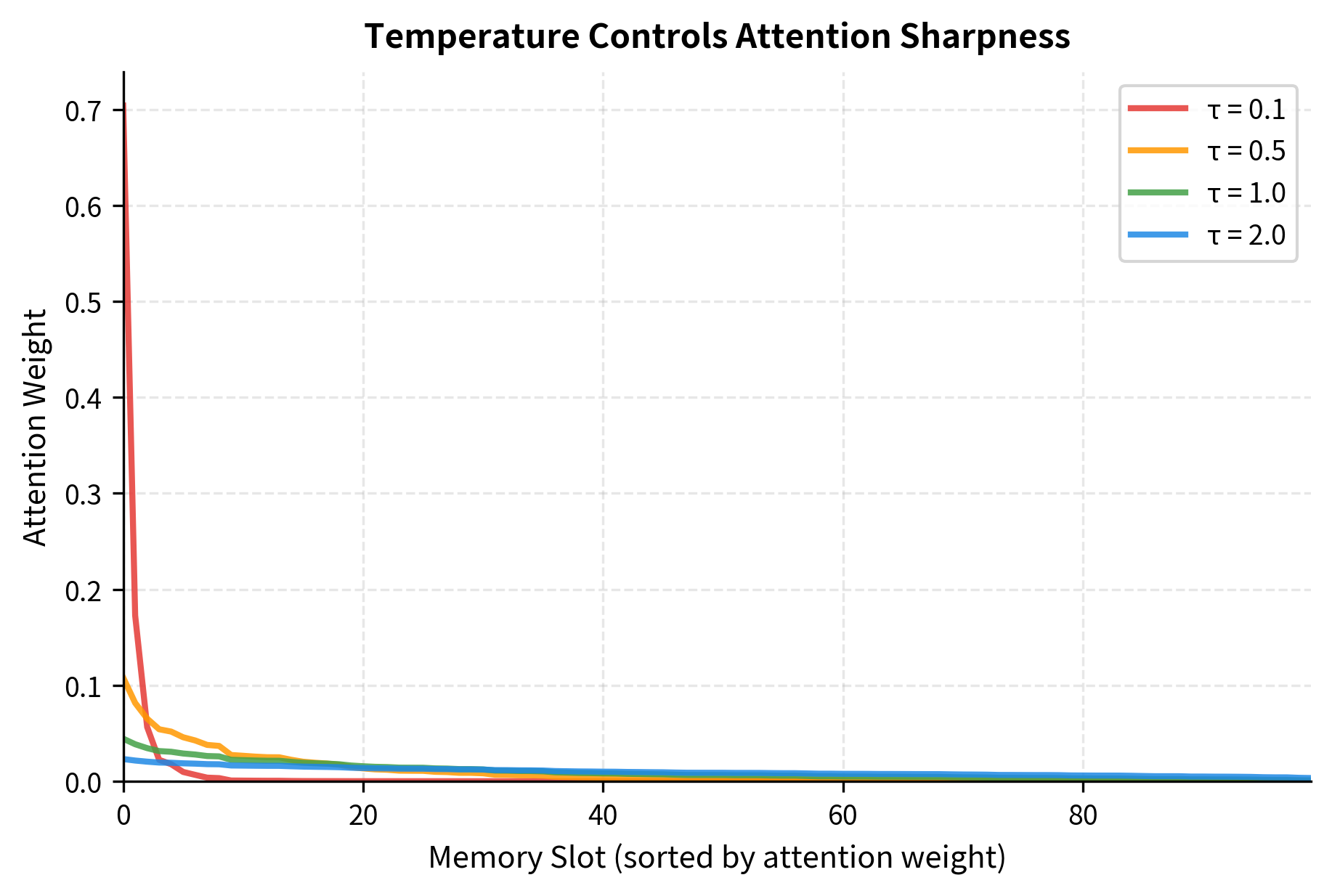
The results demonstrate the entropy-focus tradeoff concretely. At temperature 0.1, the entropy is low and the maximum weight approaches 1.0, meaning the model concentrates almost all attention on a single memory slot. The softmax has become nearly a hard argmax. At temperature 2.0, entropy increases substantially as attention spreads more evenly across slots.
This tradeoff has practical implications:
- For fact retrieval (e.g., "What is the capital of France?"), use low temperatures. The answer exists in one specific memory location.
- For synthesis tasks (e.g., "Summarize the key themes"), use higher temperatures. Relevant information is distributed across many entries.
- For training, moderate temperatures (0.5-1.0) often work best. They allow gradient flow to multiple entries without completely diluting the signal.
However, temperature alone cannot solve the scalability problem. Even with sharp attention, we still compute similarities with all memory entries. When reaches millions, this becomes prohibitively expensive.
Top-k Retrieval: Trading Differentiability for Efficiency
A more radical solution abandons the soft attention over all entries. Instead, we first find the most relevant memory slots using a discrete selection step, then apply soft attention only over those entries:
The top- operation returns the indices of the highest-scoring entries. We then compute attention only over this subset:
The key insight is that is fixed regardless of memory size . Whether the memory contains 1,000 or 1,000,000 entries, we only attend over slots in the final step. This bounds the attention computation at regardless of .
The Differentiability Tradeoff
There's a catch: the top- selection involves an argmax-like operation (finding the highest scores), which is not differentiable. During backpropagation, we cannot compute gradients through the discrete selection step.
This means entries that weren't selected receive no gradient signal, even if they were "almost" selected. The model cannot learn to make a near-miss entry more relevant. In practice, this limitation is often acceptable because:
- The entries that were selected still receive full gradients
- The key representations are typically trained with other objectives (like the main language modeling loss)
- The selection step can be approximated during training using straight-through estimators or Gumbel-softmax tricks
For many applications, the efficiency gains vastly outweigh this differentiability cost.
The efficiency gains are dramatic. With , we use only 0.05% of the memory slots for the attention computation, a 2000x reduction compared to attending to all entries. Even with for more comprehensive retrieval, we still use only 1% of the memory.
Complexity Analysis: Where the Time Goes
Let's trace through the computational costs:
- Scoring all keys: We still compute for all entries:
- Finding top-k: Selecting the largest from scores: (or for a heap-based algorithm)
- Attention over k: Softmax and weighted sum over entries:
The total is for exact top-k retrieval. We've bounded the attention step but not the scoring step.
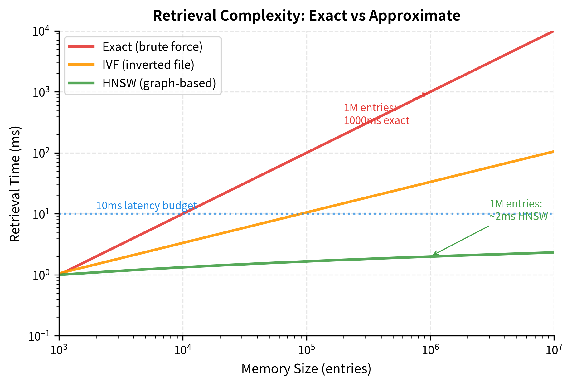
For truly large memories (millions of entries), even linear scoring becomes prohibitive. This is where approximate nearest neighbor (ANN) algorithms enter. Methods like FAISS, ScaNN, or Annoy build index structures that support sublinear retrieval:
- Exact search: to find top-k
- Approximate search: or even depending on the algorithm and acceptable accuracy loss
With ANN indexing, a memory of 1 million entries can be queried nearly as fast as a memory of 1,000 entries, at the cost of occasionally missing the truly best match.
Hierarchical Memory
Top-k retrieval solves the attention efficiency problem but treats all memory entries uniformly. When memories span multiple time scales, a more sophisticated organization helps: hierarchical memory separates recent detailed information from older compressed summaries.
Short-term memory holds recent context at full resolution, while long-term memory stores condensed representations from earlier. The model queries both levels, using short-term memory for detailed recent information and long-term memory for general patterns.
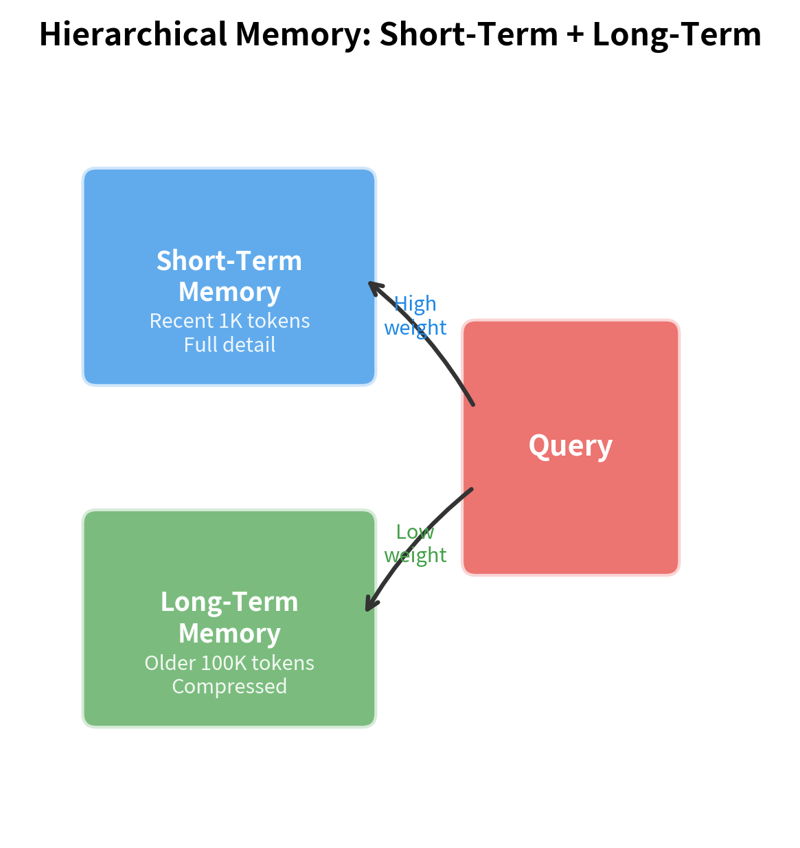
The hierarchical approach mirrors how human memory works: detailed episodic memory for recent events, condensed semantic memory for older knowledge. For language models, this translates to storing recent token representations at full resolution while compressing older context into summary vectors.
Memory Writing and Updating
Reading is only half the story. The model must also decide what to write to memory and when to update existing entries. Several strategies exist.
Append-Only Memory
The simplest approach appends new key-value pairs without modifying existing entries. This preserves all historical information but causes unbounded memory growth.
Memory usage grows linearly with tokens processed. After processing 10,000 tokens, the memory consumes approximately 0.73 MB. While this seems manageable, extrapolating to 1 million tokens would require 73 MB, and to 100 million tokens would require 7.3 GB. For long-running applications like continuous conversation or document streaming, this unbounded growth eventually exhausts available memory.
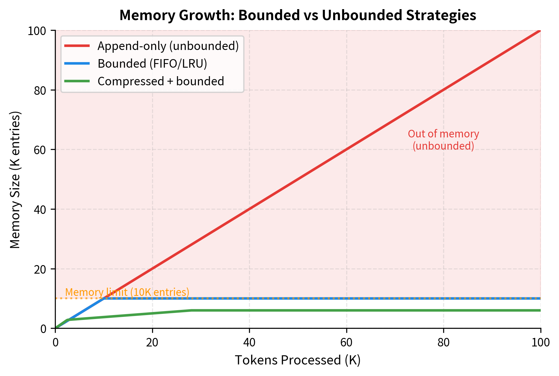
Bounded Memory with Eviction
To bound memory size, older or less-used entries must be evicted. Common strategies include FIFO (first-in, first-out), LRU (least recently used), and importance-weighted eviction.
The choice of eviction policy depends on the access patterns of your application. FIFO works well when information has a natural temporal ordering and older entries become less relevant over time. LRU is better suited for applications with "hot" entries that are accessed repeatedly, as it keeps frequently-used information available even if it was written long ago.
Learnable Writing Decisions
More sophisticated approaches learn when and what to write. A gating mechanism can control write operations based on content importance.
The gate values demonstrate learned selectivity. With the default threshold of 0.5, inputs with gate values above this threshold get written to memory while others are discarded. In this example with random initialization, the gate produces varying importance scores. After training, the gate would learn to assign high scores to information that proves useful for downstream tasks and low scores to redundant or irrelevant content.
The write gate learns to recognize important information that's worth storing. During training, the model receives gradients based on whether stored information proved useful for downstream tasks. This naturally filters out redundant or irrelevant content.
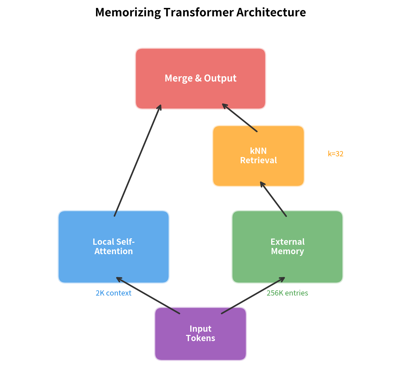
Memorizing Transformers
The Memorizing Transformer (Wu et al., 2022) represents a practical integration of external memory with transformer architecture. It extends a standard transformer by adding a -nearest neighbors (NN) retrieval mechanism that queries a large external memory during the attention computation.
In NN retrieval, given a query vector, we find the memory entries whose keys are most similar to the query (typically measured by dot product or cosine similarity). Only these entries participate in the subsequent attention computation, making retrieval efficient regardless of total memory size.
The key insight is that you can store key-value pairs from previous forward passes and retrieve them during current processing. This effectively extends context far beyond the model's native window without increasing the attention computation cost.
The memory grows with each processed chunk, accumulating key-value pairs from all previous tokens. By chunk 10, the model has seen over 10,000 tokens but only needs to store 8,192 keys in memory (bounded by the configured memory size). The effective context, which is the combination of the local window (512 tokens) plus the memory (8,192 entries), reaches 8,704 positions that the model can attend to when generating the next token.
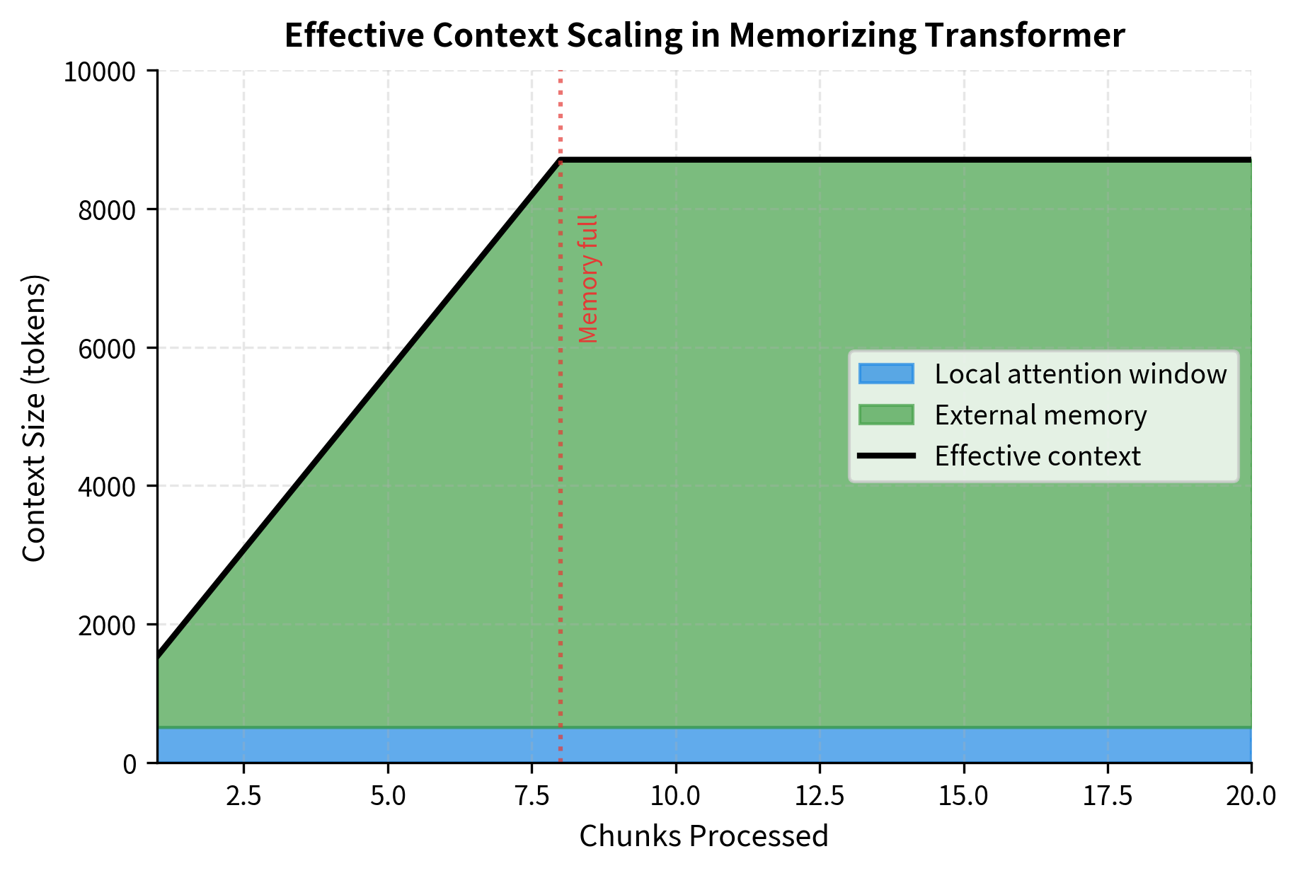
The Memorizing Transformer demonstrates how external memory scales context dramatically. After processing just 10 chunks, the model can access information from 10,000+ tokens ago while keeping each attention operation limited to a small local window plus retrieved neighbors.
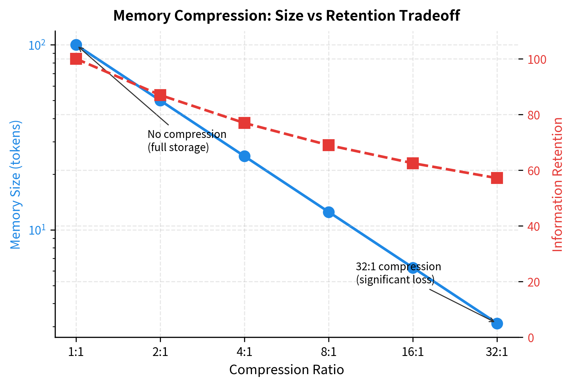
Memory Compression for Long-Term Storage
Raw storage of all past key-value pairs becomes expensive at scale. Compression techniques reduce memory footprint while preserving utility.
After writing 200 entries, the compressed memory stores only a fraction of what an uncompressed system would require. Short-term memory holds recent entries at full resolution for precise retrieval, while long-term memory contains compressed summaries that capture the essence of older entries. The achieved compression ratio demonstrates significant storage savings, though the actual information retained depends on how well the compression network learns to preserve task-relevant details.
A Worked Example: Document QA with Memory
Let's build a complete example of using memory augmentation for question answering over a long document. We'll process the document in chunks, store key information to memory, and then query that memory to answer questions.
The retrieval scores indicate how well each memory chunk matches the question. Higher scores suggest stronger relevance. For the question about height, the system successfully retrieves chunks containing the phrase "330 metres tall." The simple bag-of-characters encoding used here provides only basic matching. A production system would use learned embeddings that capture semantic similarity rather than surface-level character overlap.
The QA system demonstrates the core memory augmentation workflow: process a document into memory chunks, then query memory to find relevant context for answering questions. In a real system, the encoder would be a trained transformer, and the question answering would combine retrieved context with a generative model.
Comparing Memory Augmentation Approaches
Different memory architectures suit different use cases. Let's compare the key tradeoffs.
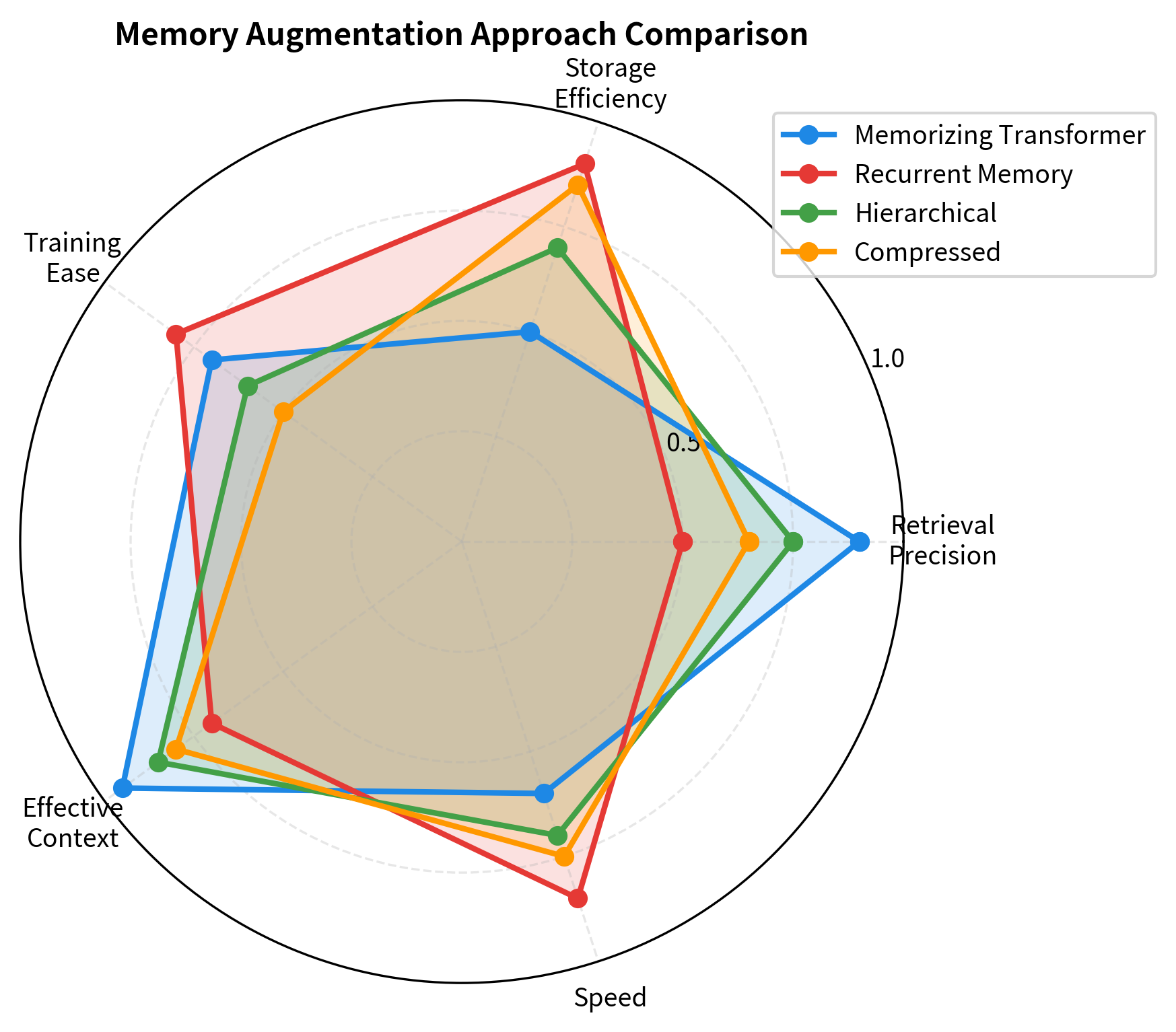
Each approach occupies a different point in the design space. Memorizing Transformers offer the best retrieval precision and effective context but require substantial storage. Recurrent memory sits at the opposite extreme with excellent storage efficiency but limited retrieval precision. Hierarchical and compressed approaches attempt to balance these tradeoffs by combining multiple memory types or using learned compression.
Key Parameters
When implementing memory-augmented models, these parameters significantly affect performance and resource usage:
| Parameter | Description | Typical Values |
|---|---|---|
memory_size | Maximum entries the memory can hold. Larger memories enable longer effective context but increase storage and retrieval costs. | 10K - 1M |
k_neighbors | Entries retrieved per query. Higher values provide more context but dilute relevance. | 4-16 (LM), 16-64 (QA) |
key_dim | Dimensionality of memory keys. Larger dimensions enable finer-grained addressing but increase compute. | 64 - 256 |
value_dim | Dimensionality of stored values. Can be larger than key_dim since values carry the actual information. | 768 - 4096 |
compression_ratio | For compressed memory, how many raw entries compress into one summary. Higher ratios save more memory but lose detail. | 4 - 16 |
temperature | Controls sharpness of retrieval attention. Lower values produce focused retrieval, higher values spread attention. | 0.1 - 2.0 |
write_gate_threshold | For gated writing, the importance threshold for storing entries. Higher thresholds mean more selective storage. | 0.3 - 0.7 |
Limitations and Considerations
Memory augmentation offers powerful capabilities but comes with significant limitations that affect practical deployment.
The fundamental challenge is the retrieval bottleneck. Even with efficient approximate nearest neighbor algorithms, querying a million-entry memory adds latency to every forward pass. For interactive applications, this overhead can dominate inference time. Batch processing helps amortize retrieval cost, but single-query latency remains a concern.
Training memory-augmented models presents its own difficulties. The memory contents change during training, creating a non-stationary optimization problem. Early in training, the memory contains noise; the model must learn to use memory while the memory itself is learning what to store. Curriculum strategies that gradually increase memory size can help, but add complexity to the training pipeline.
Storage and compute costs scale with memory size. A million-entry memory with 1024-dimensional keys and values requires approximately 8 GB of storage (assuming float32). Retrieving from this memory using exact nearest neighbors costs per query, meaning retrieval time grows linearly with the number of memory entries . For a million entries, this means scanning all million keys for each query. Approximate methods like FAISS reduce this to , where retrieval time grows only logarithmically with memory size (scanning roughly 20 entries instead of 1 million), but these methods require index maintenance and accept some retrieval accuracy loss.
The write decision problem lacks a clear solution. What should the model store? Storing everything overwhelms the memory with redundant information. Storing too selectively risks missing important details. Current approaches use heuristics (such as storing every -th token, where might be 4 or 8, to sample the input at regular intervals) or learned gates, but neither perfectly matches the downstream task's needs.
Despite these limitations, memory augmentation has proven valuable for tasks requiring precise retrieval over long contexts: document QA, knowledge-intensive generation, and personalized assistants that must remember user preferences across sessions. The key is matching the memory architecture to the task's requirements: use large, precise memories for retrieval-heavy applications; use compressed, hierarchical memories for applications that need broad context awareness without precise recall.
Summary
Memory augmentation decouples storage from computation, enabling transformers to access information beyond their native context window. The core components are:
Memory storage holds key-value pairs that the model can query. Storage strategies range from simple append-only (unbounded growth) to sophisticated compressed hierarchies (bounded size with learned summarization). The choice depends on how much historical detail the task requires.
Memory retrieval uses content-based addressing to find relevant entries. Soft attention over all entries provides differentiable training but dilutes with scale. Top-k retrieval bounds compute while sacrificing differentiability through the argmax. Temperature and control the precision-efficiency tradeoff.
Memory writing determines what enters storage. Append-only preserves everything but grows unboundedly. Eviction policies (FIFO, LRU) bound size but may discard important information. Learned gates filter based on content importance but require training signal.
Memorizing Transformers demonstrate practical integration: store key-value pairs from previous forward passes, retrieve relevant pairs during current processing, and combine retrieved context with local attention. This architecture enables effective context of hundreds of thousands of tokens while keeping each attention operation tractable.
The memory augmentation paradigm represents a fundamental shift from "remember implicitly through weights" to "remember explicitly in storage." This separation enables models that can process book-length documents, maintain conversation history across sessions, and access vast knowledge bases without compressing everything into a fixed-size hidden state.
Quiz
Ready to test your understanding? Take this quick quiz to reinforce what you've learned about memory augmentation for transformers.

Comments