Span Corruption: T5's Pretraining Objective for Sequence-to-Sequence Learning

Masked language modeling (MLM) trains models to predict individual tokens hidden behind [MASK] placeholders. But what if we masked entire phrases or multi-word expressions instead? Span corruption takes this idea further: rather than masking isolated tokens, it corrupts contiguous spans of text and asks the model to reconstruct them. This simple shift fundamentally changes what the model learns during pretraining.

T5 (Text-to-Text Transfer Transformer) popularized span corruption as its primary pretraining objective. By treating the corrupted input as source text and the original spans as target text, T5 frames pretraining as a sequence-to-sequence problem. This approach produces models that excel at generation tasks while remaining competitive on understanding benchmarks.

In this chapter, you'll learn how span corruption works, why it outperforms token-level masking for certain applications, and how to implement it from scratch. We'll cover span selection strategies, the mathematics of span length distributions, sentinel token design, and the computational advantages that make this approach attractive at scale.

Standard MLM randomly selects 15% of tokens and replaces them with [MASK]. The model predicts each masked token independently, using the surrounding context. This works well but has limitations.

Consider the phrase "the cat sat on the mat." If MLM masks "sat" and "mat" independently, the model makes two separate predictions. It never learns that these words might be related or that predicting multi-word expressions requires different reasoning than predicting single tokens.

Span corruption addresses this by masking contiguous sequences. Instead of the [MASK] sat on the [MASK], we might see the [X] on [Y] where [X] replaces "cat sat" and [Y] replaces "the mat." The model must now generate complete phrases, not isolated words.

This shift has several consequences. First, the input sequence becomes shorter because multiple tokens collapse into single sentinels. Second, the target sequence contains multiple tokens per sentinel, requiring the model to generate coherently. Third, the model learns about phrase-level patterns and dependencies that token-level masking might miss.

Now that we understand what span corruption does conceptually, we need to answer a practical question: how do we decide which parts of a sequence to corrupt? This leads us to two interconnected design choices that significantly affect what the model learns.

Think of span corruption as a controlled demolition. We want to remove enough of the building (the text) to create a meaningful reconstruction challenge, but not so much that the remaining structure provides no clues about what was removed. This balance requires careful decisions about two quantities: how much total material to remove (the corruption rate) and how to divide that material into chunks (the span length distribution).

The corruption rate $r$ specifies what fraction of the original tokens should end up inside corrupted spans. T5 adopts $r = 0.15$, matching BERT's masking rate, but the mechanics differ substantially from token-level masking.

In standard MLM, a 15% corruption rate means we independently flip a coin for each token, with 15% probability of masking. The result: exactly 15% of tokens become [MASK], scattered throughout the sequence. With span corruption, we instead select contiguous regions totaling approximately 15% of the sequence. The key difference is that these tokens are grouped, not isolated.

This grouping creates an interesting constraint. If we want to corrupt a fixed fraction of tokens, the number of spans we create depends on how long each span is. Suppose we have a sequence of $n$ tokens and want to corrupt fraction $r$ of them. If each span contains an average of $\mu$ tokens, simple arithmetic tells us how many spans we need:

where:

• $n$: the total number of tokens in the input sequence
• $r$: the corruption rate (fraction of tokens to corrupt, e.g., 0.15 for 15%)
• $\mu$: the average span length (e.g., 3 tokens per span)

The reasoning is direct: we need to "cover" $r \cdot n$ tokens with our spans. If each span covers $\mu$ tokens on average, we need $(r \cdot n) / \mu$ spans to achieve the target coverage.

Let's make this concrete. For a 512-token sequence with $r = 0.15$ and $\mu = 3$:

1. Tokens to corrupt: $0.15 \times 512 \approx 77$ tokens
2. Spans needed: $77 / 3 \approx 26$ spans
3. Input length after corruption: Each span gets replaced by one sentinel token, so the corrupted input contains $512 - 77 + 26 = 461$ tokens

This calculation reveals an important property: span corruption naturally compresses the input sequence. We remove 77 tokens but add only 26 sentinels, achieving a net reduction of 51 tokens (about 10% shorter). This compression has computational benefits we'll explore later.

The corruption rate tells us how much to remove; the span length distribution tells us how to partition that removal into individual spans. This choice significantly affects what patterns the model learns.

Consider the extremes. If all spans had length 1, span corruption would collapse to token-level masking: we'd have 77 isolated masks, each predicting a single token independently. If all spans had length 77, we'd have one massive gap containing over half the sequence, providing almost no useful training signal.

The sweet spot lies somewhere between. We want a mix of span lengths that exposes the model to diverse reconstruction challenges: some single-token predictions (maintaining fine-grained language modeling ability), some short phrases (learning local coherence), and occasional longer spans (forcing the model to reason about larger structures).

T5 uses a geometric distribution to achieve this mix. The geometric distribution is the discrete analog of the exponential distribution, modeling a natural process: imagine flipping a biased coin at each position within a span, continuing until we get "heads" (stop) instead of "tails" (continue). The span length equals how many positions we visited before stopping.

Mathematically, if the probability of stopping at each step is $p$, the probability of a span having exactly $\ell$ tokens is:

where:

• $P(\ell)$: the probability of sampling a span of exactly $\ell$ tokens
• $\ell$: the span length (a positive integer: 1, 2, 3, ...)
• $p$: the stopping probability at each step, controlling the distribution's shape
• $(1 - p)^{\ell - 1}$: the probability of "continuing" for $\ell - 1$ steps before finally "stopping"

This formula captures a simple generative process: to get a span of length $\ell$, we need $\ell - 1$ consecutive "continue" decisions (each with probability $1 - p$) followed by one "stop" decision (with probability $p$).

The geometric distribution has a convenient property: its mean equals $1/p$. This gives us a direct way to control the average span length. If we want spans to average $\mu$ tokens, we simply set:

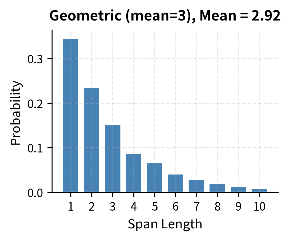
For T5's choice of $\mu = 3$, this gives $p = 1/3$. At each step within a span, there's a 1-in-3 chance of stopping. The resulting distribution strongly favors shorter spans while maintaining a "heavy tail" of longer ones:

• $P(\ell = 1) = 0.33$ (one-third of spans are single tokens)
• $P(\ell = 2) = 0.22$ (about one-fifth are two tokens)
• $P(\ell = 3) = 0.15$ (around one-sixth are three tokens)
• $P(\ell = 4) = 0.10$ (one-tenth are four tokens)
• $P(\ell \geq 5) = 0.20$ (about one-fifth contain five or more tokens)

This distribution creates a rich training curriculum. The model frequently encounters single-token predictions, maintaining its vocabulary knowledge. It regularly sees two and three-token spans, learning common phrases and local syntax. And it occasionally faces longer spans requiring genuine compositional reasoning.

Let's visualize this distribution by sampling 10,000 span lengths and plotting the empirical frequencies. This will confirm our theoretical calculations and reveal the characteristic exponential decay.

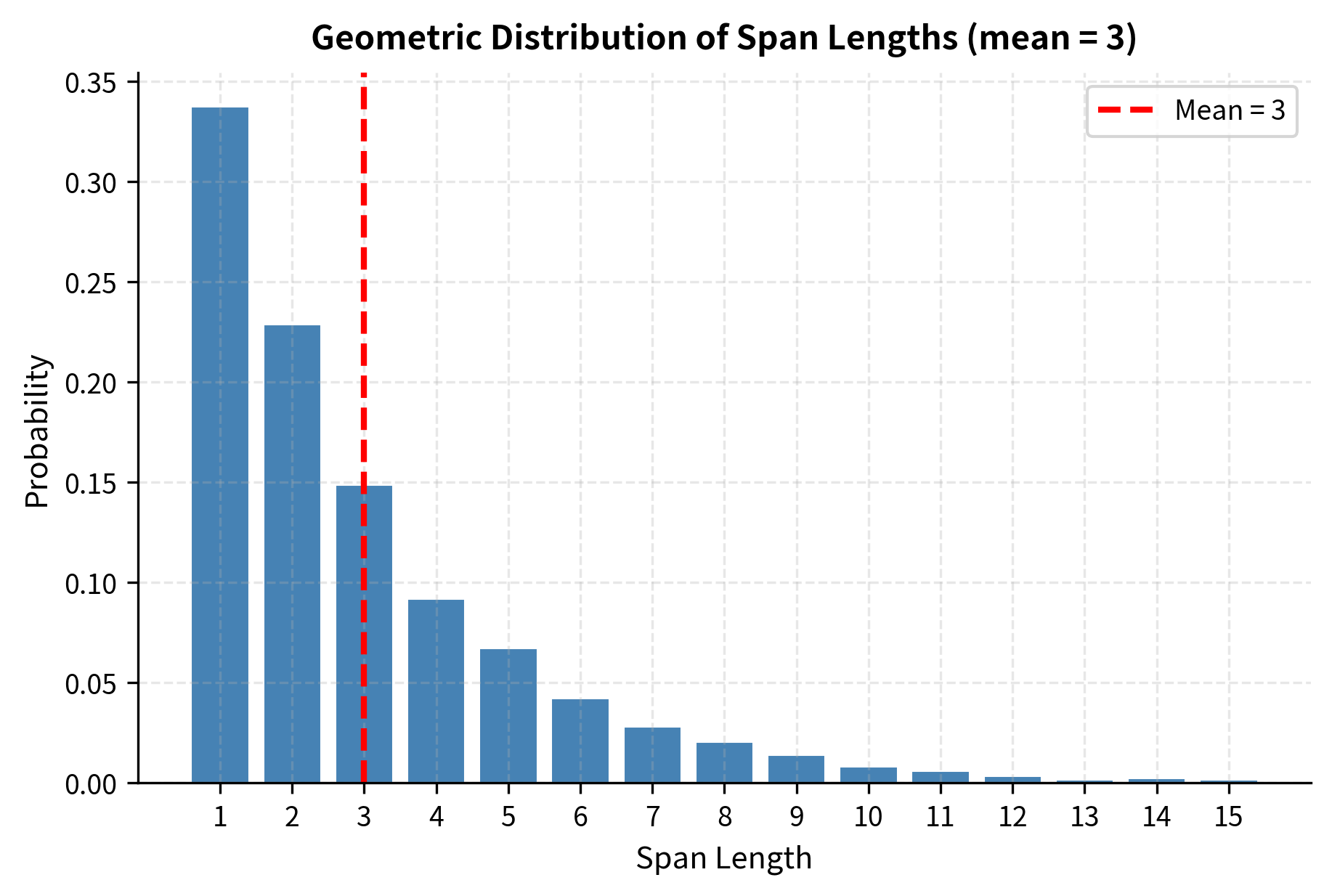
The empirical distribution matches our theoretical expectations. Notice the characteristic exponential decay: each bar is roughly two-thirds the height of the previous one (since $(1-p) = 2/3$). The red dashed line marks the mean at 3, which falls slightly to the right of the mode (1), reflecting the distribution's right skew.

Why does this shape work well for pretraining? The geometric distribution provides a natural curriculum:

1. High-frequency short spans maintain the model's ability to predict individual tokens accurately, preserving fine-grained vocabulary knowledge
2. Medium-length spans teach local coherence and common phrases, the bread-and-butter of fluent text generation
3. The heavy tail occasionally challenges the model with longer reconstructions, forcing it to reason about syntax, entities, and discourse structure

This is more effective than a uniform distribution, which would waste equal capacity on trivially short spans and overwhelmingly long ones. The geometric decay concentrates learning where it's most useful while still providing exposure to diverse span lengths.

Another way to understand the distribution is through the cumulative perspective: what fraction of spans have length at most $\ell$? This cumulative distribution function (CDF) answers practical questions like "what percentage of spans are single tokens?" or "how often do we see spans longer than 5 tokens?"

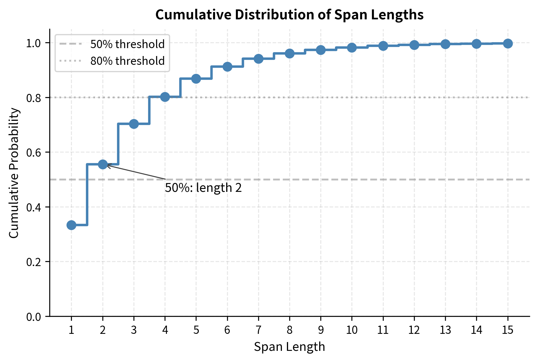
The CDF reveals that roughly half of all spans have length 2 or less, and about 80% have length 4 or less. Only the remaining 20% challenge the model with longer reconstructions. This steep rise followed by a gradual tail perfectly balances frequent short-span practice with occasional longer challenges.

Sentinel tokens serve as placeholders for corrupted spans. Unlike BERT's single [MASK] token, span corruption uses multiple distinct sentinels, typically denoted <extra_id_0>, <extra_id_1>, and so on.

Why use different sentinels for each span? Consider reconstructing two spans from the corrupted input. If both used the same [MASK] token, the model couldn't distinguish which output corresponds to which span. Distinct sentinels create a clear mapping between input positions and output targets.

The target sequence concatenates all corrupted spans, each preceded by its corresponding sentinel:

Original: "The quick brown fox jumps over the lazy dog"

Corrupted Input: "The <extra_id_0> fox <extra_id_1> lazy dog"

Target: "<extra_id_0> quick brown <extra_id_1> jumps over the"

This format enables autoregressive generation of the target. The model sees <extra_id_0> and generates "quick brown" before the next sentinel signals a new span.

T5's vocabulary reserves 100 sentinel tokens (<extra_id_0> through <extra_id_99>). This typically suffices since even long sequences rarely contain more than 50-60 spans with a 15% corruption rate and average span length of 3.

Now that we understand the mathematics behind span selection, let's translate these concepts into working code. We'll build the algorithm incrementally, starting from the core span selection logic and gradually assembling the complete corruption pipeline. By the end, you'll have a clear picture of how each formula we derived connects to the implementation.

Our first task is to decide which token positions fall within corrupted spans. We need an algorithm that:

1. Determines how many spans to create (using our formula: $\approx r \cdot n / \mu$)
2. Samples each span's length from a geometric distribution
3. Places spans at random positions without overlap

We'll represent the result as a corruption mask: a boolean array where True indicates that token should be part of some corrupted span.

The visualization shows corrupted positions as filled blocks (█) and uncorrupted positions as empty blocks (░). Notice how the corrupted tokens cluster into contiguous groups rather than scattering randomly across the sequence. This is the defining characteristic of span corruption: tokens within each span will be replaced by a single sentinel and reconstructed together.

With approximately 15% of tokens corrupted, we've created distinct "holes" in the sequence that the model must learn to fill. The spans vary in length according to our geometric distribution, some containing just one or two tokens, others stretching across several positions.

The corruption mask tells us which positions are corrupted, but for the next step we need to know where each span begins and ends. This boundary information lets us replace each contiguous span with exactly one sentinel token and extract the corresponding target tokens.

The algorithm finds each contiguous run of True values in the mask. Each span gets a unique index (0, 1, 2, ...) that will serve as its identifier when we assign sentinel tokens. Notice how span lengths vary: some spans contain just one token, others two or three, following our geometric distribution.

With span boundaries identified, we can now construct the two sequences that define the training example:

1. Corrupted input: The original sequence with each span replaced by its sentinel token (e.g., <extra_id_0>, <extra_id_1>)
2. Target sequence: A concatenation of all corrupted spans, each preceded by its corresponding sentinel

This format creates a clear mapping: the model sees a sentinel in the input and learns to generate the corresponding tokens in the target.

Let's see this in action with a real sentence:

Examine the output carefully. The corrupted input is noticeably shorter than the original: multi-token spans have collapsed into single sentinel tokens. The target sequence contains exactly the tokens that were removed, each group prefixed by its sentinel to maintain the correspondence.

This structure shows how span corruption works in practice. The model must:

1. Understand context: Use the uncorrupted tokens surrounding each sentinel to infer what's missing
2. Generate coherently: Produce complete phrases, not just isolated words, for each sentinel
3. Maintain boundaries: Know when one span ends and the next begins, guided by the sentinel markers

With all the pieces in place, let's combine them into a reusable class that encapsulates the full span corruption logic:

The results confirm our earlier calculations. The original 14-token sequence becomes a 12-token corrupted input (the corruption plus sentinels compress the sequence) and a compact target containing only the corrupted material plus sentinel markers.

This completes our span corruption implementation. Starting from the mathematical foundations, we've built each component:

1. Span count estimation: $(r \cdot n) / \mu$ spans needed for the target corruption rate
2. Length sampling: Geometric distribution with $p = 1/\mu$ for natural length variation
3. Boundary detection: Linear scan to identify contiguous corrupted regions
4. Sequence construction: Parallel building of input (with sentinels) and target (spans preceded by sentinels)

The algorithm is efficient, running in linear time relative to sequence length, and produces the exact format expected by T5-style encoder-decoder training.

T5 uses span corruption within an encoder-decoder framework. The corrupted input feeds into the encoder, while the decoder autoregressively generates the target sequence. This setup naturally handles variable-length span reconstruction.

The encoder processes the corrupted input sequence, producing hidden representations that capture the context around each sentinel:

where:

• $H_{\text{enc}}$: the encoder's output hidden states, a matrix of shape (sequence length $\times$ hidden dimension)
• $x_1, \ldots, x_n$: the corrupted input tokens, including uncorrupted tokens and sentinel placeholders
• $\text{<extra\_id\_0>}$: a sentinel token marking where a span was removed

The decoder then generates the target sequence autoregressively, conditioned on the encoder's hidden states:

where:

• $y_t$: the token being predicted at position $t$ in the target sequence
• $y_{<t}$: all previously generated target tokens $(y_1, y_2, \ldots, y_{t-1})$
• $P(y_t \mid y_{<t}, H_{\text{enc}})$: the probability distribution over the vocabulary for the next token

During training, we use teacher forcing: the decoder receives the true previous tokens rather than its own predictions. The training objective is standard cross-entropy loss over the target sequence:

where:

• $\mathcal{L}$: the total loss for this training example
• $T$: the length of the target sequence
• $\log P(y_t \mid \cdot)$: the log probability assigned to the correct token at each position

This loss encourages the model to assign high probability to the actual tokens that were corrupted, learning to reconstruct spans from context.

Span corruption works well with encoder-decoder models because:

• Bidirectional encoding: The encoder sees all uncorrupted context simultaneously, enabling rich representations of what surrounds each sentinel.
• Autoregressive decoding: The decoder generates spans token by token, learning proper phrase structure and coherence.
• Natural length handling: Spans of different lengths produce targets of different lengths, which encoder-decoder models handle gracefully.

Decoder-only models can also use span corruption, treating the task as infilling. The corrupted input and target concatenate with appropriate separators, and the model learns to continue after each sentinel.

Let's compare the training signals from span corruption versus token-level MLM:

With MLM, each mask corresponds to exactly one token. With span corruption, each sentinel may require generating multiple tokens, forcing the model to learn phrase-level coherence.

The difference becomes clearer when we visualize the corruption patterns side by side. Let's create multiple samples and compare how MLM scatters masks across the sequence while span corruption creates contiguous blocks.

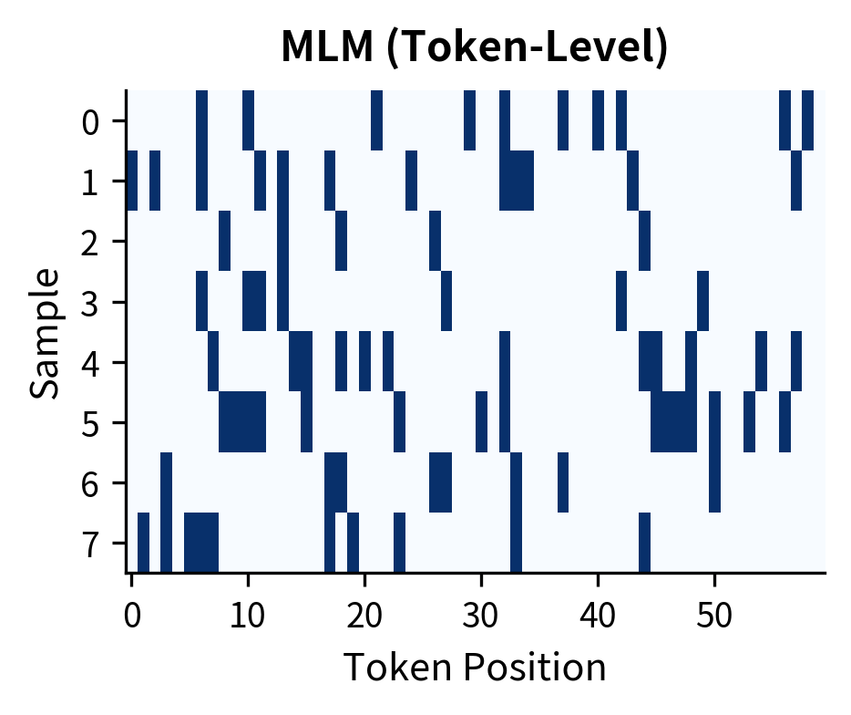
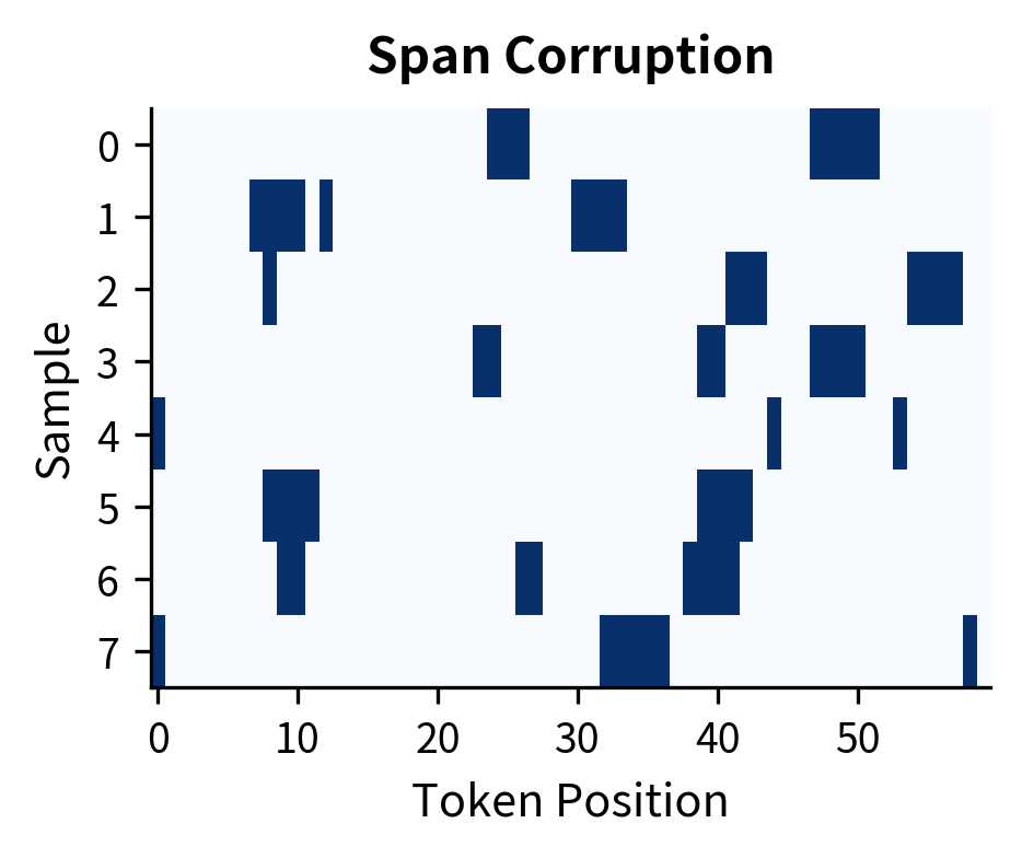
The visual contrast is clear. MLM produces a scattered, salt-and-pepper pattern where each dark cell is an isolated prediction task. Span corruption creates horizontal streaks, each representing a multi-token reconstruction challenge. This structural difference explains why span-corrupted models develop stronger phrase-level generation capabilities.

Researchers have explored several variations of the basic span corruption approach.

While T5 uses geometric distribution, some work explores uniform distributions. With uniform sampling between 1 and $k$, every span length up to $k$ is equally likely:

Geometric distributions produce more short spans but allow occasional long ones. Uniform distributions guarantee exposure to longer spans but may waste capacity on trivially short reconstructions.

We can also explore how different mean span lengths affect the distribution shape. Higher means produce flatter distributions with more emphasis on longer spans.

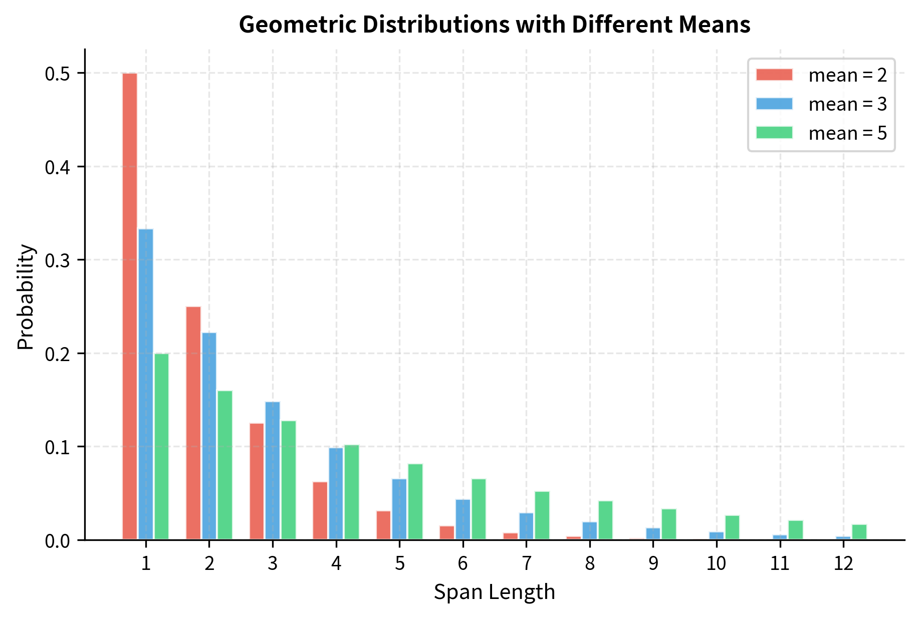
With $\mu = 2$, nearly half of all spans are single tokens, providing mostly token-level signal. With $\mu = 5$, the distribution flattens significantly, exposing the model to longer spans more frequently but at the cost of fewer distinct spans per sequence. T5's choice of $\mu = 3$ balances these extremes.

The original T5 paper tested corruption rates from 10% to 50%. Higher rates create shorter inputs but longer targets:

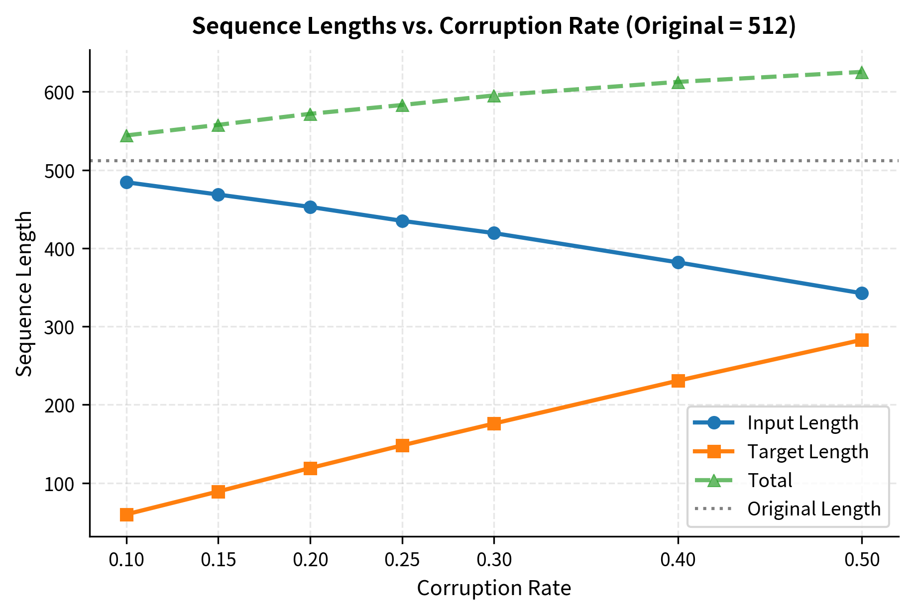
At 15% corruption, the input shrinks modestly while the target remains manageable. Higher rates shift more content to the target, which can slow training due to longer autoregressive generation.

Some models combine span corruption with prefix language modeling. The uncorrupted prefix receives bidirectional attention, while corrupted spans use causal attention:

Input: "The quick brown" + <extra_id_0> + "jumps over" + <extra_id_1>

Attention:

• "The quick brown": Bidirectional (full visibility)
• Sentinels and after: Causal (left-to-right only)

This hybrid approach lets the model leverage bidirectional context for understanding while maintaining generative capability.

Span corruption offers surprising computational advantages over token-level masking.

Because multiple tokens collapse into single sentinels, the encoder processes fewer tokens. For a 512-token sequence with 15% corruption and mean span length 3:

• Original tokens corrupted: ~77 tokens
• Sentinels added: ~26 tokens
• Net input length: ~461 tokens (10% reduction)

This reduction compounds across the quadratic attention mechanism. Attention cost scales as $O(n^2)$, where $n$ is the sequence length. A 10% length reduction (from $n$ to $0.9n$) yields roughly 19% savings in attention computation, since $(0.9)^2 = 0.81$.

The target sequence contains only corrupted spans plus sentinels. With 15% corruption:

• Target length: ~77 (spans) + ~26 (sentinels) = ~103 tokens

The decoder processes 103 tokens instead of 512, dramatically reducing generation cost during training.

Let's quantify the computational savings:

Let's visualize these computational trade-offs across different corruption rates to understand when span corruption provides the greatest efficiency gains.

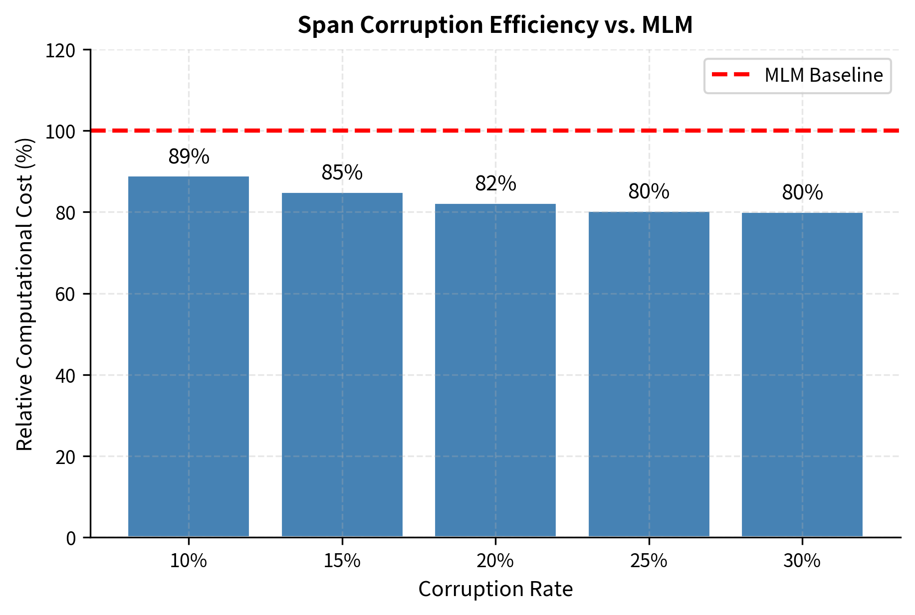
Span corruption achieves meaningful computational savings while still exposing the model to diverse reconstruction challenges. At the standard 15% corruption rate, we save roughly 15% of computation compared to MLM. The encoder sees nearly the full context (minus corrupted tokens), while the decoder focuses only on what needs reconstruction.

Span corruption offers compelling benefits, but it comes with trade-offs that affect model behavior and downstream applications.

The most significant limitation is the mismatch between pretraining and generation tasks. During pretraining, the model learns to infill missing spans given surrounding context. During generation, the model must produce text autoregressively without such scaffolding. This gap means span-corrupted models may struggle with open-ended generation compared to models pretrained with causal language modeling. T5 addresses this partially by framing all tasks as text-to-text, but the underlying tension remains. Fine-tuning helps bridge the gap, yet models pretrained exclusively on span corruption often require more adaptation for generation-heavy applications.

Another consideration is span boundary artifacts. The model learns that sentinels mark span boundaries, potentially creating implicit assumptions about phrase structure. If spans happen to align with linguistic units (noun phrases, clauses), the model may learn useful structure. If spans cut through units arbitrarily, the model must learn to handle artificial boundaries. The random nature of span selection means both cases occur, which may introduce noise into the learned representations.

Key practical limitations include:

• Sentinel token overhead: Each span requires a unique sentinel, consuming vocabulary space and adding tokens to both input and target sequences.
• Span length sensitivity: Very short spans (length 1) resemble MLM without the multi-prediction benefit. Very long spans remove too much context for reliable reconstruction.
• Reconstruction ambiguity: When spans contain common phrases, multiple valid reconstructions may exist, yet training penalizes all but the original.

Despite these limitations, span corruption works well in practice. T5 and its variants achieve strong performance across diverse benchmarks, suggesting that the benefits of efficient training and phrase-level learning outweigh the costs.

When implementing span corruption, the following parameters have the greatest impact on training behavior and model performance:

• corruption_rate (float, default: 0.15): Fraction of tokens to include in corrupted spans. Higher rates (0.3-0.5) create more challenging reconstruction tasks but produce longer targets that slow training. Lower rates (0.1) may underutilize the model's capacity. The T5 default of 0.15 balances learning signal with computational efficiency.

• mean_span_length (int, default: 3): Controls the average number of tokens per corrupted span via the geometric distribution parameter $p = 1/\mu$. Shorter spans (mean 1-2) behave like token-level masking. Longer spans (mean 5+) force phrase-level generation but reduce the number of distinct spans. A mean of 3 provides good coverage of both short and medium-length phrases.

• num_sentinels (int, default: 100): Maximum number of unique sentinel tokens available. This caps the number of spans per sequence. With a 15% corruption rate and mean span length of 3, a 512-token sequence produces ~26 spans, well within the default limit. Increase only for very long sequences or high corruption rates.

• span_length_distribution (str, options: "geometric", "uniform"): Geometric distributions favor shorter spans with occasional long ones, matching T5's approach. Uniform distributions guarantee equal exposure to all span lengths within a range but may waste capacity on trivially short reconstructions.

Span corruption extends masked language modeling by corrupting contiguous token spans rather than individual tokens. Key takeaways:

• Span selection: Geometric distributions with mean 3 balance short and long spans, exposing the model to both token-level and phrase-level reconstruction.
• Sentinel tokens: Unique sentinels (<extra_id_0>, <extra_id_1>, ...) replace each span, creating a clear mapping between input positions and target outputs.
• Sequence-to-sequence framing: The corrupted input becomes the encoder source; concatenated spans with sentinels become the decoder target.
• Computational efficiency: Shorter input and target sequences reduce attention costs, making training more efficient than full-sequence objectives.
• Trade-offs: The infilling objective may not transfer perfectly to open-ended generation, requiring careful fine-tuning for generation tasks.

Span corruption powers T5 and influenced subsequent models like UL2 and PaLM, which explore mixtures of denoising objectives. Understanding this technique provides insight into how pretraining objectives shape model capabilities and efficiency.

Ready to test your understanding? Take this quick quiz to reinforce what you've learned about span corruption and T5-style pretraining.