Search

Search articles

Autoregressive Generation: How GPT Generates Text Token by Token

Michael BrenndoerferUpdated July 30, 202555 min read

Master the mechanics of autoregressive generation in transformers, including the generation loop, KV caching for efficiency, stopping criteria, and speed optimizations for production deployment.

Track your reading progress

Sign in to mark chapters as read and track your learning journey

Sign in →
Reading Level

Choose your expertise level to adjust how many terms are explained. Beginners see more tooltips, experts see fewer to maintain reading flow. Hover over underlined terms for instant definitions.

Autoregressive Generation

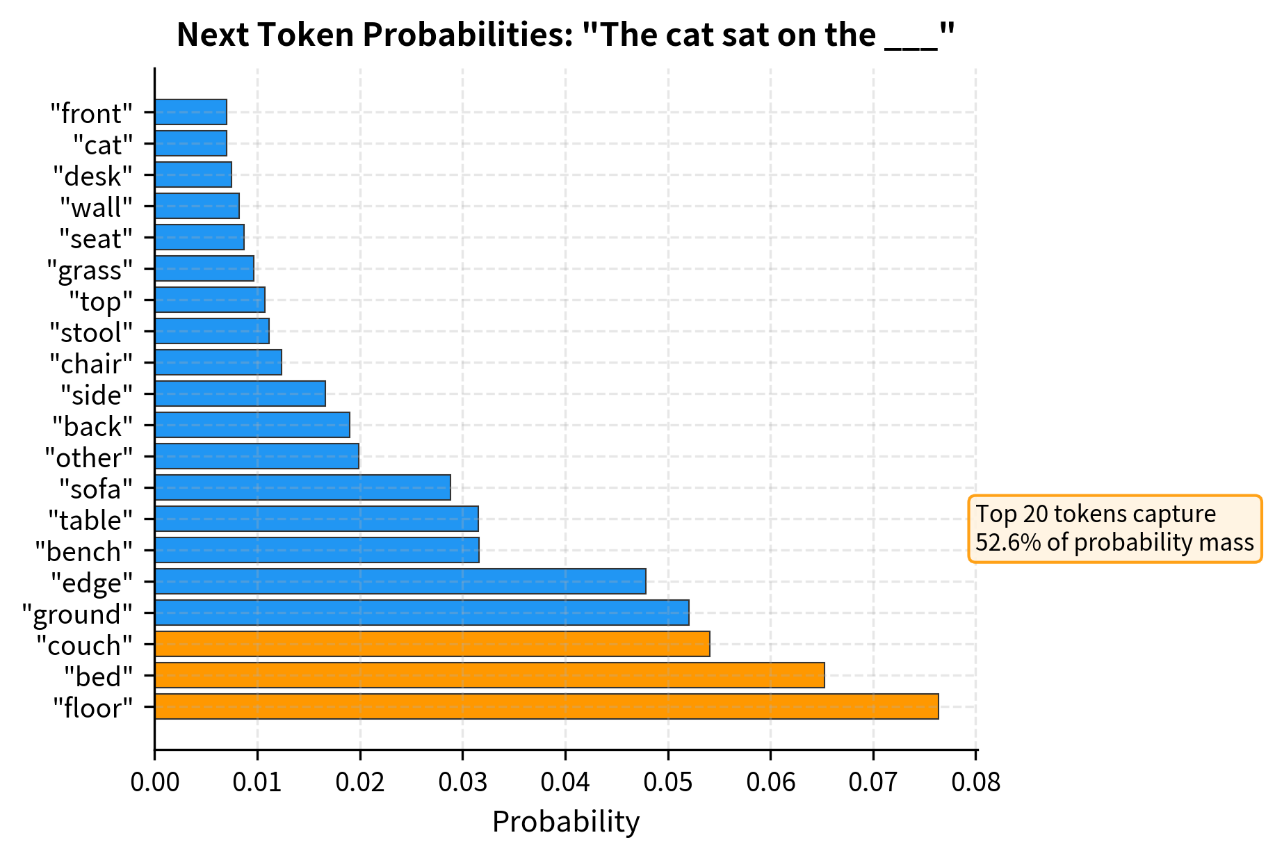
When you ask a language model to complete the sentence "The cat sat on the", it doesn't produce the entire response at once. Instead, it generates text one token at a time, each new token conditioned on all the tokens that came before. This process, called autoregressive generation, is the fundamental mechanism by which decoder-only transformers like GPT produce coherent, contextually appropriate text.

Understanding autoregressive generation is essential for working with modern language models. The process seems simple on the surface: predict the next token, append it to the sequence, and repeat. But underneath this simple loop lies a computational challenge that has driven significant research into efficiency optimizations. The key insight is that naive generation would recompute the same attention calculations repeatedly, wasting enormous amounts of compute. The solution, key-value caching, transforms generation from quadratically expensive to linearly efficient.

This chapter explores the mechanics of autoregressive generation in detail. We'll implement the generation loop from scratch, understand why KV caching is crucial for practical deployment, examine stopping criteria that determine when generation ends, and explore techniques for optimizing generation speed. By the end, you'll understand not just how to call a generation function, but how generation actually works inside the model.

The Generation Procedure

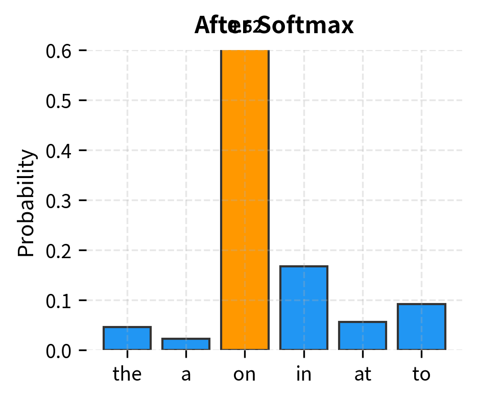
Autoregressive generation follows a straightforward principle: at each step, the model predicts a probability distribution over possible next tokens, selects one token from that distribution, appends it to the sequence, and repeats until some stopping condition is met.

Autoregressive Generation

Autoregressive generation produces sequences token-by-token, where each new token is conditioned on all previously generated tokens. The probability of generating a complete sequence factorizes as P(x1,,xn)=i=1nP(xix1,,xi1)P(x_1, \ldots, x_n) = \prod_{i=1}^{n} P(x_i | x_1, \ldots, x_{i-1}), meaning we multiply together the probability of each token given everything that came before it.

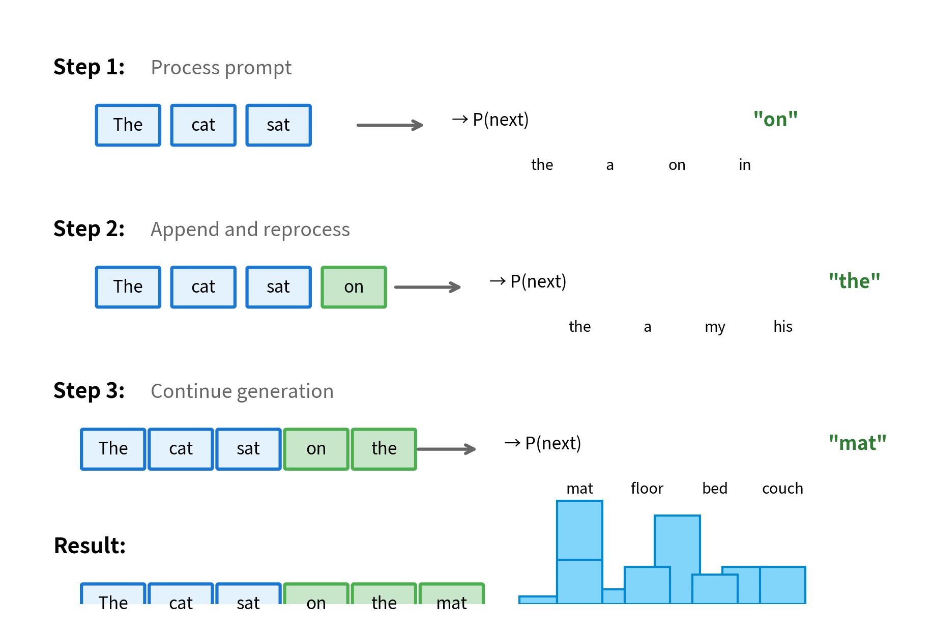
The process begins with a prompt, which is a sequence of tokens provided by the user. The model processes this prompt to produce hidden states, then uses the final hidden state to predict the first generated token. This token is appended to the prompt, the model processes the extended sequence, and the cycle continues.

In[3]:
Code
def greedy_generate(model, tokenizer, prompt: str, max_new_tokens: int = 50):
    """
    Generate text using greedy decoding (always pick the most likely token).

    This is the simplest generation strategy: at each step, select the token
    with the highest probability.
    """
    # Encode the prompt
    input_ids = tokenizer.encode(prompt, return_tensors="pt")

    # Generate tokens one at a time
    for _ in range(max_new_tokens):
        # Forward pass through the model
        with torch.no_grad():
            outputs = model(input_ids)
            logits = outputs.logits

        # Get logits for the last position
        next_token_logits = logits[:, -1, :]

        # Greedy selection: pick the highest probability token
        next_token_id = next_token_logits.argmax(dim=-1, keepdim=True)

        # Append to the sequence
        input_ids = torch.cat([input_ids, next_token_id], dim=1)

        # Check for end of sequence
        if next_token_id.item() == tokenizer.eos_token_id:
            break

    # Decode and return the generated text
    return tokenizer.decode(input_ids[0], skip_special_tokens=True)

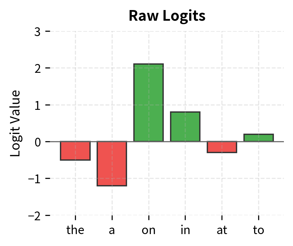
This implementation reveals several important aspects of generation. First, the model produces logits (unnormalized log-probabilities) for every position in the vocabulary at once. We only use the logits at the final position since that's where the next token prediction happens. Second, greedy decoding, which always selects the most probable token, is deterministic: the same prompt always produces the same output. Third, the loop continues until we either reach max_new_tokens or generate an end-of-sequence token.

Out[5]:
Console
Prompt: The future of artificial intelligence
Generated: The future of artificial intelligence is uncertain.

"We're not sure what the future will look like," said Dr. Michael S. Schoenfeld, a professor of

The generated continuation flows naturally from the prompt, demonstrating that the model has learned meaningful language patterns. Notice how each word follows logically from the previous context. Greedy decoding often produces repetitive or generic text because it always takes the safe, high-probability path. We'll explore more sophisticated sampling strategies in subsequent chapters on temperature, top-k sampling, and nucleus sampling. For now, the key insight is that all generation strategies share the same underlying loop: predict, select, append, repeat.

Out[6]:
Visualization
Horizontal bar chart showing the top 20 most probable next tokens, with floor and ground having the highest probabilities around 0.10-0.12.
Top-20 token probabilities after processing 'The cat sat on the'. The model assigns highest probability to 'floor' and 'ground', reflecting common language patterns. Most of GPT-2's 50,257 vocabulary tokens receive near-zero probability, concentrating the mass on contextually appropriate completions.

The Generation Loop in Detail

Let's trace through exactly what happens at each step of generation. Consider a simple 4-token vocabulary and a prompt of 3 tokens:

Out[7]:
Visualization
Diagram showing three iterations of the generation loop with growing sequences and probability distributions.
The autoregressive generation loop. At each step, the model processes the current sequence to produce logits, selects the next token, and appends it. The sequence grows by one token per iteration until a stopping criterion is met.

At each step, the model must process the entire sequence to maintain the correct attention patterns. The attention mechanism at position ii computes weighted sums over all positions jij \leq i, so earlier tokens influence later predictions. This creates a computational challenge: as the sequence grows, each forward pass becomes more expensive.

Mathematical Formulation

The generation loop we've been exploring raises a fundamental question: how do we assign a probability to an entire sequence of tokens? Consider the sentence "The cat sat on the mat". It would be impractical to maintain a probability table for every possible sentence, as natural language allows infinitely many valid sequences. Instead, we need a way to decompose sequence probability into manageable pieces.

From Intuition to the Chain Rule

Think about how you might estimate the likelihood of a sentence. You wouldn't evaluate it as a monolithic unit. Instead, you'd naturally consider: How likely is "The" as an opening word? Given that we started with "The", how likely is "cat" to follow? Given "The cat", how likely is "sat"? This intuitive approach of building probability step by step is exactly what autoregressive models formalize.

The mathematical foundation comes from the chain rule of probability, which states that any joint probability can be decomposed into a product of conditional probabilities. For a sequence of TT tokens, this gives us the autoregressive factorization:

P(x1,x2,,xT)=t=1TP(xtx1,x2,,xt1)P(x_1, x_2, \ldots, x_T) = \prod_{t=1}^{T} P(x_t | x_1, x_2, \ldots, x_{t-1})

where:

  • xtx_t: the token at position tt in the sequence
  • TT: the total sequence length (number of tokens)
  • P(xtx1,x2,,xt1)P(x_t | x_1, x_2, \ldots, x_{t-1}): the conditional probability of token xtx_t given all preceding tokens, often written as P(xtx<t)P(x_t | x_{<t}) for brevity
  • t=1T\prod_{t=1}^{T}: the product over all positions from 1 to TT

This factorization is powerful because it transforms the impossible task of modeling all possible sentences into a tractable one: we only need to model what comes next given what we've seen so far. Each factor in the product corresponds to exactly one step of the generation loop.

A Concrete Example

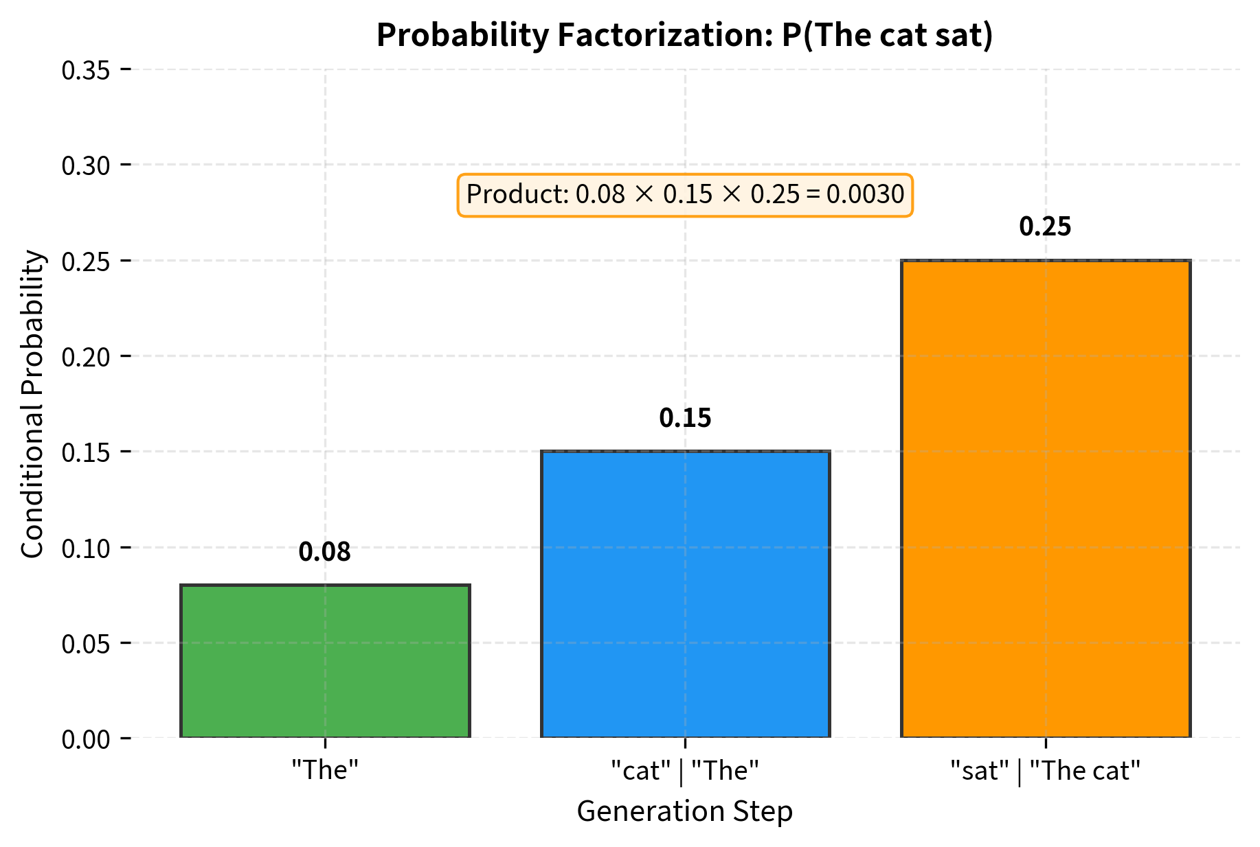
Let's trace through the factorization for our example sentence "The cat sat":

  1. First token: P("The")P(\text{"The"}) asks how likely "The" is as an opening. Common sentence starters like "The", "A", "I" receive high probability.

  2. Second token: P("cat""The")P(\text{"cat"} | \text{"The"}) asks what noun is likely after "The". Words like "cat", "dog", "man", "house" all receive some probability mass.

  3. Third token: P("sat""The cat")P(\text{"sat"} | \text{"The cat"}) asks what action a cat might perform. "sat", "jumped", "ran", "slept" become likely candidates.

The full sequence probability is the product: P("The")×P("cat""The")×P("sat""The cat")P(\text{"The"}) \times P(\text{"cat"} | \text{"The"}) \times P(\text{"sat"} | \text{"The cat"}). If any factor is near zero, the entire product collapses, reflecting that an unlikely transition makes the whole sequence improbable.

Out[8]:
Visualization
Bar chart showing conditional probabilities for each token in the sequence The cat sat, with probability values decreasing from left to right.
Autoregressive probability factorization for ''The cat sat''. Each bar shows the conditional probability at that step. The sequence probability is the product of all factors: 0.08 × 0.15 × 0.25 = 0.003, meaning this specific three-word sequence appears in about 0.3% of contexts where ''The'' could start a sentence.

From Hidden States to Probabilities

Now we need to understand how the model actually computes each conditional probability P(xtx<t)P(x_t | x_{<t}). This happens in two stages:

  1. Encode the context: The transformer processes all tokens x1,,xt1x_1, \ldots, x_{t-1} to produce a hidden state hth_t that summarizes the relevant context.

  2. Project to vocabulary: A linear layer maps this hidden state to a score for every token in the vocabulary, then softmax converts these scores to probabilities.

The formula for this computation is:

P(xtx<t)=softmax(Wlmht+b)xtP(x_t | x_{<t}) = \text{softmax}(W_{\text{lm}} \cdot h_t + b)_{x_t}

where:

  • htRdh_t \in \mathbb{R}^{d}: the hidden state vector at position tt from the final transformer layer, where dd is the hidden dimension (e.g., 768 for GPT-2 Small). This vector encodes everything the model "knows" about the context so far.
  • WlmRV×dW_{\text{lm}} \in \mathbb{R}^{V \times d}: the language modeling head weight matrix that projects from hidden dimension to vocabulary size VV. Each row of this matrix can be thought of as a "template" for one vocabulary token.
  • bRVb \in \mathbb{R}^{V}: the bias term (often zero or absent in modern implementations), which captures token-independent frequency preferences.
  • softmax()xt\text{softmax}(\cdot)_{x_t}: the probability assigned to token xtx_t after normalization.

The product WlmhtW_{\text{lm}} \cdot h_t computes a score (logit) for each vocabulary token by measuring how similar the current context representation is to each token's template. Higher scores indicate more likely next tokens. The softmax function then performs two crucial operations:

  1. Exponentiation (ezie^{z_i}) ensures all values become positive
  2. Normalization (dividing by the sum) ensures probabilities sum to 1
Out[9]:
Visualization
Raw logits can be any real number. Negative logits (red) indicate less likely tokens, while positive logits (green) indicate more likely ones. The token 'on' has the highest logit at 2.1.
After softmax, logits become probabilities that sum to 1.0. The token 'on' receives the highest probability (0.52) because it had the highest logit.

Why Generation Must Be Sequential

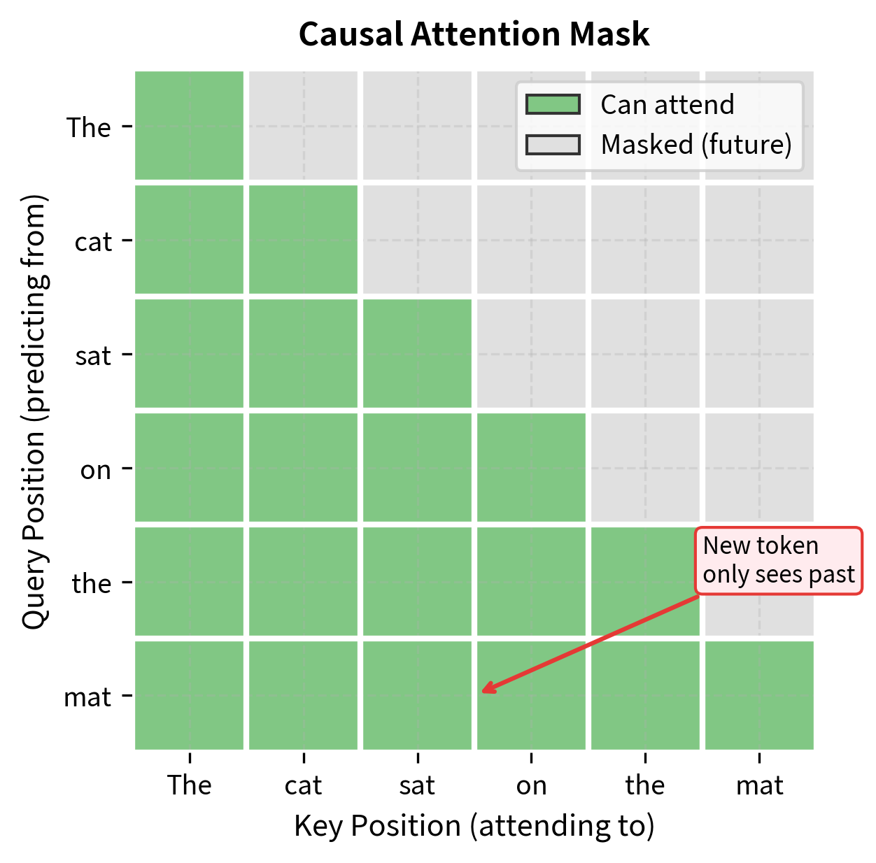
This mathematical structure reveals a fundamental constraint: we cannot parallelize generation across positions. To compute hth_t, the model must know tokens x1,,xt1x_1, \ldots, x_{t-1}, because the transformer's causal attention mask prevents each position from seeing future tokens.

Concretely, if we want to predict the 10th token:

  • We need h10h_{10}, the hidden state at position 10
  • Computing h10h_{10} requires attention over positions 1 through 9
  • But positions 1 through 9 must contain actual tokens, not placeholders
  • Therefore, we must have already generated tokens 1 through 9

This sequential dependency is what makes autoregressive generation inherently step-by-step. Unlike tasks like classification where we process the entire input in parallel, generation must proceed one token at a time, with each new token depending on all previous decisions.

Out[10]:
Visualization
Heatmap showing a lower triangular attention mask where green cells indicate allowed attention and gray cells indicate masked future positions.
Causal attention mask enforcing the autoregressive property. Each position can only attend to itself and earlier positions (green cells). Future positions are masked (gray cells). This triangular structure ensures the model cannot 'cheat' by looking ahead during generation.

Why Naive Generation is Expensive

Consider generating 100 tokens after a 50-token prompt. With naive generation, each step requires a full forward pass through the model. The first generated token requires processing 50 tokens. The second requires processing 51 tokens. The hundredth requires processing 149 tokens.

The total computation scales quadratically with sequence length because attention at each position must attend to all previous positions. To see why, consider that at generation step ii, we must compute attention over a sequence of length ii. The total number of attention operations across all TT generation steps is:

Total attention operationsi=1Ti=T(T+1)2=O(T2)\text{Total attention operations} \propto \sum_{i=1}^{T} i = \frac{T(T+1)}{2} = O(T^2)

where:

  • TT: the total number of tokens generated
  • i=1Ti\sum_{i=1}^{T} i: the sum of sequence lengths processed at each step (1 + 2 + 3 + ... + T)
  • T(T+1)2\frac{T(T+1)}{2}: the closed-form solution for this arithmetic series
  • O(T2)O(T^2): big-O notation indicating quadratic growth with sequence length

This quadratic relationship means that generating 1000 tokens requires roughly 1,000,000 attention operations proportionally, while generating just 100 tokens requires only about 10,000. The cost grows much faster than the output length.

Out[11]:
Visualization
Line plot showing quadratic growth of attention operations with sequence length for naive generation.
Computational cost of naive autoregressive generation. Each step requires recomputing attention over the entire sequence, leading to quadratic growth. For a 1000-token generation, the naive approach performs over 500,000 attention operations versus 1000 with proper caching.

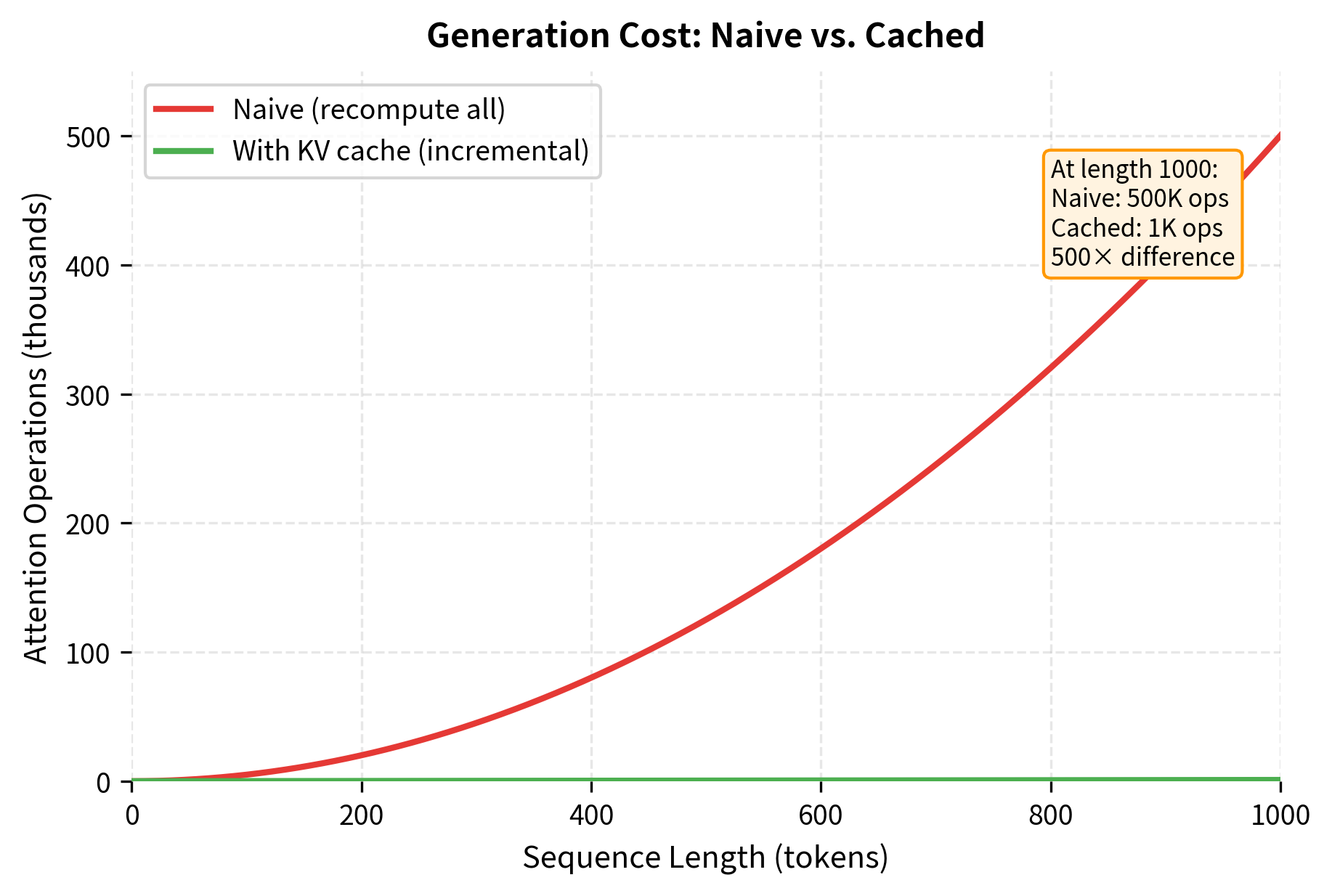
For practical deployments where latency matters, this quadratic scaling is unacceptable. Generating a single response could take tens of seconds even on powerful hardware. The solution is to cache intermediate computations and reuse them across generation steps.

Key-Value Caching

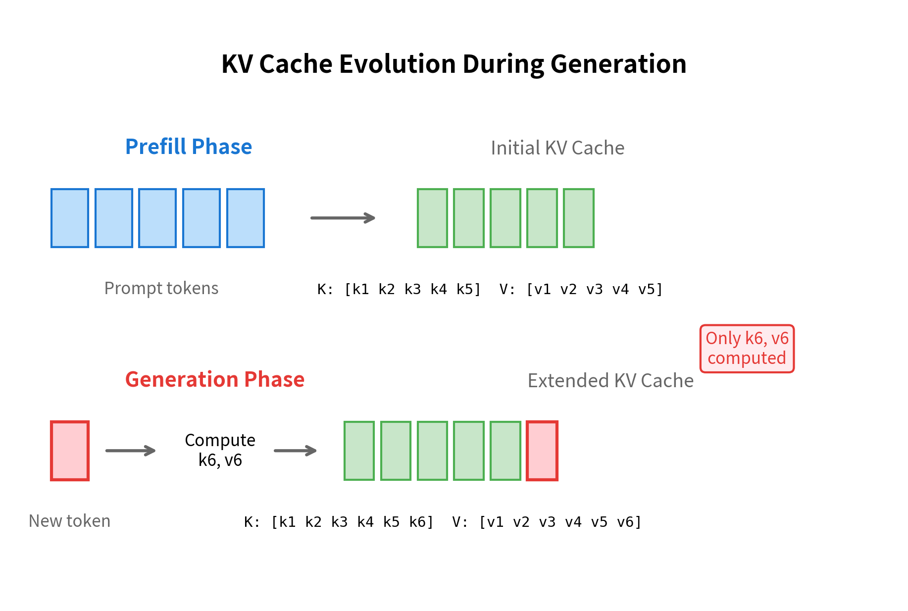
The key insight behind KV caching is that during autoregressive generation, the attention keys and values for positions 1 through t1t-1 don't change when we generate token tt. Only the new token at position tt introduces new keys and values. Instead of recomputing everything, we cache the keys and values from previous positions and only compute the new entries.

KV Cache

The KV cache stores the key and value projections from each attention layer for all previously processed tokens. During generation, only the new token's keys and values are computed and appended to the cache, avoiding redundant computation.

How Attention Works Without Caching

To understand why KV caching helps, we first need to understand what happens in standard attention. In multi-head attention, for a sequence of length TT, we compute queries, keys, and values from the input, then use them to compute a weighted sum:

Attention(Q,K,V)=softmax(QKTdk)V\text{Attention}(Q, K, V) = \text{softmax}\left(\frac{QK^T}{\sqrt{d_k}}\right)V

where:

  • QRT×dkQ \in \mathbb{R}^{T \times d_k}: the query matrix containing a query vector for each of the TT positions
  • KRT×dkK \in \mathbb{R}^{T \times d_k}: the key matrix containing a key vector for each position
  • VRT×dvV \in \mathbb{R}^{T \times d_v}: the value matrix containing a value vector for each position
  • dkd_k: the dimension of each key (and query) vector, typically 64 in GPT-2
  • QKTRT×TQK^T \in \mathbb{R}^{T \times T}
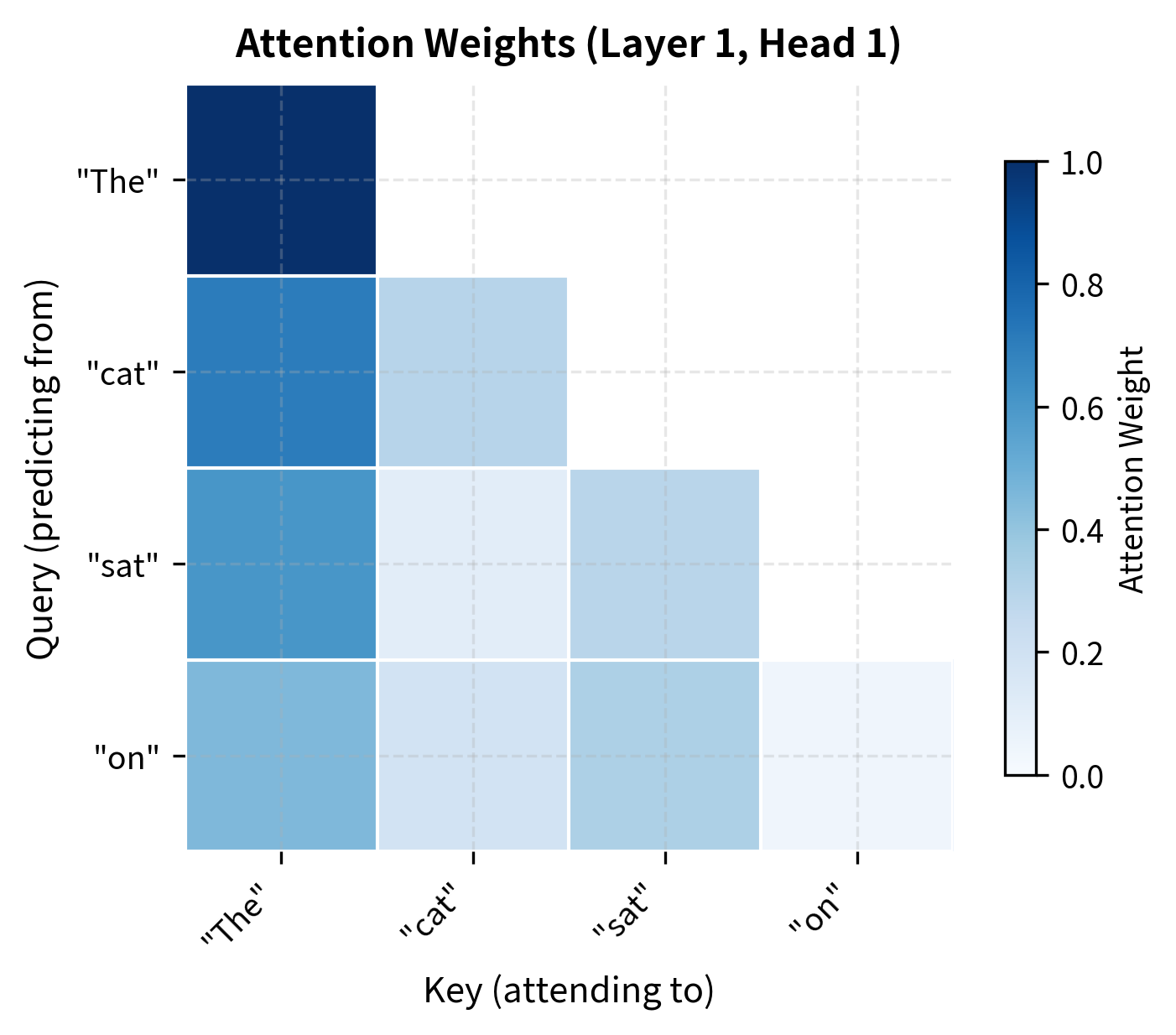
: the attention score matrix where entry (i,j)(i, j) measures how much position ii attends to position jj
  • dk\sqrt{d_k}: a scaling factor that prevents the dot products from growing too large, which would push softmax into regions with vanishing gradients
  • softmax()\text{softmax}(\cdot): normalizes each row of the attention scores to sum to 1, creating attention weights

The formula works in three steps: (1) compute attention scores by taking dot products between queries and keys, (2) normalize scores with softmax to get attention weights, and (3) compute weighted sums of values using those weights.

During generation, we actually only need the query at the last position to predict the next token. But without caching, we must recompute the entire KK and VV matrices at every step because the attention mechanism requires all previous keys and values to compute the softmax normalization correctly.

How Attention Works With Caching

With KV caching, we maintain running matrices KcacheK_{\text{cache}} and VcacheV_{\text{cache}} that accumulate the keys and values for all tokens processed so far. When generating token tt:

  1. Compute only qtq_t, ktk_t, vtv_t for the new token (a single vector each)
  2. Append ktk_t to KcacheK_{\text{cache}} and vtv_t to VcacheV_{\text{cache}} (cache grows by one row)
  3. Compute attention using qtq_t (single query) against the full cache

The attention computation for the new token becomes:

Attention(qt,Kcache,Vcache)=softmax(qtKcacheTdk)Vcache\text{Attention}(q_t, K_{\text{cache}}, V_{\text{cache}}) = \text{softmax}\left(\frac{q_t K_{\text{cache}}^T}{\sqrt{d_k}}\right)V_{\text{cache}}

where:

  • qtR1×dkq_t \in \mathbb{R}^{1 \times d_k}: the query vector for the single new token at position tt
  • KcacheRt×dkK_{\text{cache}} \in \mathbb{R}^{t \times d_k}: the cached key matrix containing keys for all tt positions seen so far
  • VcacheRt×dvV_{\text{cache}} \in \mathbb{R}^{t \times d_v}: the cached value matrix containing values for all tt positions
  • qtKcacheTR1×tq_t K_{\text{cache}}^T \in \mathbb{R}^{1 \times t}: a single row of attention scores (the new token attending to all previous positions)
  • dk\sqrt{d_k}: the same scaling factor as before

The key insight is that qtKcacheTq_t K_{\text{cache}}^T produces just a single row of attention scores rather than a full T×TT \times T matrix. We compute tt dot products instead of t2t^2, reducing the per-step computation from O(T2)O(T^2) to O(T)O(T). Over the full generation of TT tokens, this changes the total cost from O(T3)O(T^3) to O(T2)O(T^2), a dramatic improvement for long sequences.

Out[12]:
Visualization
Heatmap showing attention weights from GPT-2 with darker colors indicating stronger attention, displaying a lower-triangular pattern due to causal masking.
Actual attention weights from GPT-2's first layer for 'The cat sat on'. Each row shows how a token distributes its attention across previous positions. Later tokens can attend to all earlier tokens but not future ones. The 'on' token attends strongly to 'sat' (the verb it modifies) and 'The' (the sentence start).
In[13]:
Code
import torch.nn as nn


class CachedAttention(nn.Module):
    """Multi-head attention with KV caching for efficient generation."""

    def __init__(self, hidden_size: int = 768, num_heads: int = 12):
        super().__init__()
        self.hidden_size = hidden_size
        self.num_heads = num_heads
        self.head_dim = hidden_size // num_heads

        self.q_proj = nn.Linear(hidden_size, hidden_size)
        self.k_proj = nn.Linear(hidden_size, hidden_size)
        self.v_proj = nn.Linear(hidden_size, hidden_size)
        self.out_proj = nn.Linear(hidden_size, hidden_size)

    def forward(
        self,
        hidden_states: torch.Tensor,
        past_key_value: tuple[torch.Tensor, torch.Tensor] | None = None,
        use_cache: bool = True,
    ) -> tuple[torch.Tensor, tuple[torch.Tensor, torch.Tensor] | None]:
        batch_size, seq_len, _ = hidden_states.shape

        # Project queries, keys, values
        q = self.q_proj(hidden_states)
        k = self.k_proj(hidden_states)
        v = self.v_proj(hidden_states)

        # Reshape for multi-head attention
        q = q.view(
            batch_size, seq_len, self.num_heads, self.head_dim
        ).transpose(1, 2)
        k = k.view(
            batch_size, seq_len, self.num_heads, self.head_dim
        ).transpose(1, 2)
        v = v.view(
            batch_size, seq_len, self.num_heads, self.head_dim
        ).transpose(1, 2)

        # Handle KV cache
        if past_key_value is not None:
            # Append new keys and values to cache
            past_k, past_v = past_key_value
            k = torch.cat([past_k, k], dim=2)
            v = torch.cat([past_v, v], dim=2)

        # Store updated cache
        present_key_value = (k, v) if use_cache else None

        # Compute attention scores
        attn_weights = torch.matmul(q, k.transpose(-2, -1)) / (
            self.head_dim**0.5
        )

        # Apply causal mask
        total_len = k.size(2)
        query_len = q.size(2)
        causal_mask = torch.triu(
            torch.ones(query_len, total_len, device=q.device),
            diagonal=total_len - query_len + 1,
        ).bool()
        attn_weights = attn_weights.masked_fill(causal_mask, float("-inf"))

        attn_weights = F.softmax(attn_weights, dim=-1)

        # Apply attention to values
        attn_output = torch.matmul(attn_weights, v)

        # Reshape and project output
        attn_output = attn_output.transpose(1, 2).contiguous()
        attn_output = attn_output.view(batch_size, seq_len, self.hidden_size)
        attn_output = self.out_proj(attn_output)

        return attn_output, present_key_value
Out[14]:
Console
After prompt (10 tokens):
  Output shape: torch.Size([1, 10, 256])
  Cached K shape: torch.Size([1, 4, 10, 64])
  Cached V shape: torch.Size([1, 4, 10, 64])

After generating 1 token:
  Input shape: torch.Size([1, 1, 256]) (single token)
  Output shape: torch.Size([1, 1, 256])
  Cached K shape: torch.Size([1, 4, 11, 64]) (now 11 positions)

The cache has grown from 10 to 11 positions after processing a single new token. Notice that the input to this step was just one token, not the entire sequence of 11. This is the efficiency gain: we only compute the new keys and values while reusing all previously cached entries.

The shapes reveal the broader efficiency principle. After the initial prompt, each generation step only processes a single token, but the cache grows to include all previous positions. The attention computation uses the single-token query against the full key cache.

Memory Implications

KV caching trades memory for computation. We gain speed by storing intermediate results, but this requires additional GPU memory that grows with sequence length. Understanding this trade-off is essential for deploying models with long context windows.

For a model with LL layers, HH attention heads per layer, head dimension dd, batch size BB, and sequence length TT, the total cache memory requirement is:

Cache memory=2×L×B×H×d×T×sizeof(dtype)\text{Cache memory} = 2 \times L \times B \times H \times d \times T \times \text{sizeof(dtype)}

where:

  • 22: accounts for storing both keys and values (two tensors per layer)
  • LL: number of transformer layers (each layer has its own cache)
  • BB: batch size (number of sequences being generated in parallel)
  • HH: number of attention heads per layer
  • dd: dimension of each head (typically dmodel/Hd_{\text{model}} / H)
  • TT: current sequence length (grows during generation)
  • sizeof(dtype)\text{sizeof(dtype)}: bytes per element (4 for float32, 2 for float16/bfloat16)

The product H×dH \times d equals the model's hidden dimension dmodeld_{\text{model}}, so we can also write this as 2×L×B×dmodel×T×sizeof(dtype)2 \times L \times B \times d_{\text{model}} \times T \times \text{sizeof(dtype)}. The key insight is that cache memory grows linearly with both model depth LL and sequence length TT.

For GPT-2 Small (12 layers, 12 heads, 64-dimensional heads, giving dmodel=768d_{\text{model}} = 768) with float16 precision:

Out[15]:
Console
KV Cache Memory Requirements (GPT-2 Small, batch=1, float16):
--------------------------------------------------
  Sequence length   512:   18.0 MB
  Sequence length  1024:   36.0 MB
  Sequence length  2048:   72.0 MB
  Sequence length  4096:  144.0 MB
  Sequence length  8192:  288.0 MB

For larger models, cache requirements grow proportionally:
  GPT-3 175B at 2048 tokens: 9.0 GB

These numbers reveal a key practical constraint. For GPT-2 Small, cache requirements remain modest even at 8K tokens. But for production-scale models like GPT-3, the cache alone consumes multiple gigabytes. When serving many concurrent users, cache memory often becomes the limiting factor before model weights.

Out[16]:
Visualization
Line plot showing KV cache memory in GB versus sequence length for three model sizes: GPT-2 Small, GPT-2 XL, and GPT-3 175B, with GPT-3 showing dramatically steeper growth.
KV cache memory requirements across model sizes and sequence lengths. Larger models with longer contexts require substantially more cache memory. At 4096 tokens, GPT-3's cache alone exceeds 4 GB, often exceeding the model weights' memory footprint in relative terms.

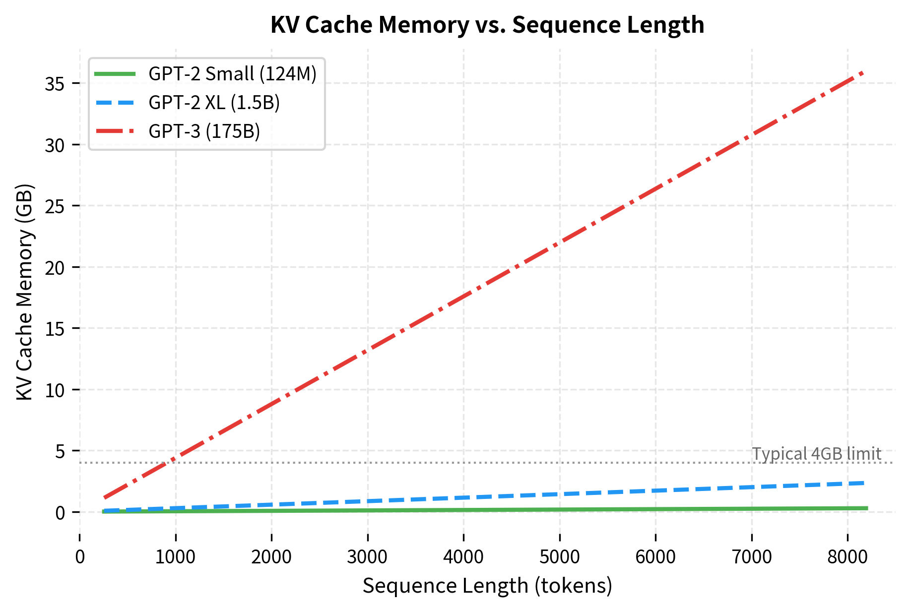
For very long sequences or large batch sizes, the KV cache can become a significant memory bottleneck. This has motivated research into cache compression, sparse attention patterns, and other memory-efficient generation techniques.

Out[17]:
Visualization
Diagram showing KV cache growing from prompt processing through token generation steps.
KV cache growth during generation. The prompt is processed once (prefill phase), populating the initial cache. Each subsequent token only adds one key-value pair per layer, enabling efficient incremental computation.

Implementation with Full Model

Let's implement efficient generation with KV caching using the Hugging Face transformers library, which handles cache management automatically:

In[18]:
Code
def efficient_generate(
    model,
    tokenizer,
    prompt: str,
    max_new_tokens: int = 50,
    temperature: float = 1.0,
):
    """
    Generate text using KV caching for efficiency.

    The model's generate method handles caching internally, but we can also
    manage it explicitly for more control.
    """
    input_ids = tokenizer.encode(prompt, return_tensors="pt")
    attention_mask = torch.ones_like(input_ids)

    # Initialize cache as None
    past_key_values = None

    generated_ids = input_ids.clone()

    for _ in range(max_new_tokens):
        with torch.no_grad():
            # Only pass new tokens if we have a cache
            if past_key_values is not None:
                # Only process the last token
                current_input = generated_ids[:, -1:]
            else:
                # First pass: process entire prompt
                current_input = generated_ids

            outputs = model(
                input_ids=current_input,
                attention_mask=attention_mask,
                past_key_values=past_key_values,
                use_cache=True,
            )

            # Update cache for next iteration
            past_key_values = outputs.past_key_values

            # Get logits for the last position
            logits = outputs.logits[:, -1, :]

            # Apply temperature
            if temperature != 1.0:
                logits = logits / temperature

            # Sample from distribution
            probs = F.softmax(logits, dim=-1)
            next_token = torch.multinomial(probs, num_samples=1)

            # Append to generated sequence
            generated_ids = torch.cat([generated_ids, next_token], dim=1)
            attention_mask = torch.cat(
                [
                    attention_mask,
                    torch.ones((1, 1), dtype=attention_mask.dtype),
                ],
                dim=1,
            )

            # Check for end of sequence
            if next_token.item() == tokenizer.eos_token_id:
                break

    return tokenizer.decode(generated_ids[0], skip_special_tokens=True)
Out[19]:
Console
Naive generation: 0.758s
Cached generation: 0.369s
Speedup: 2.1×

Generated text:
The key to understanding transformers is to have the right kind of experience for their use. That is, unless, for instance, you use them in situations that it is natural to be

The cached version runs faster because it avoids recomputing keys and values for the entire sequence at each step. For this short 30-token generation, the speedup may appear modest, but it grows substantially with sequence length. At 1000 tokens, the difference becomes orders of magnitude.

Out[20]:
Visualization
Line plot comparing generation time in seconds versus number of tokens generated, showing quadratic growth for naive approach and linear growth for cached approach.
Generation time scaling with and without KV caching. Naive generation shows quadratic growth because each step reprocesses the entire sequence. Cached generation grows linearly since each step only processes the new token. The gap widens dramatically at longer sequence lengths.

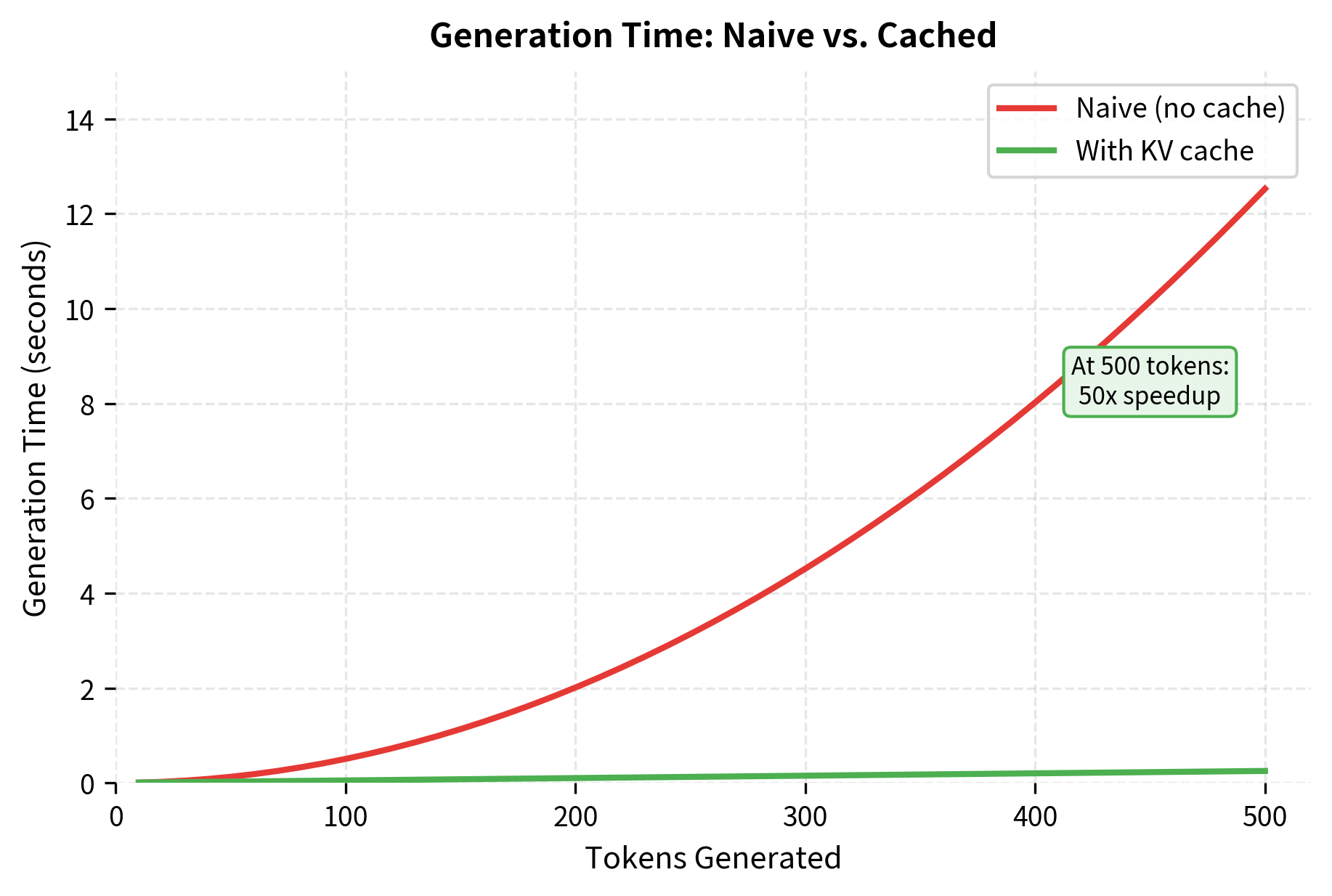
The speedup from KV caching becomes more pronounced with longer sequences. For production deployments, cached generation is essential for acceptable latency.

Stopping Criteria

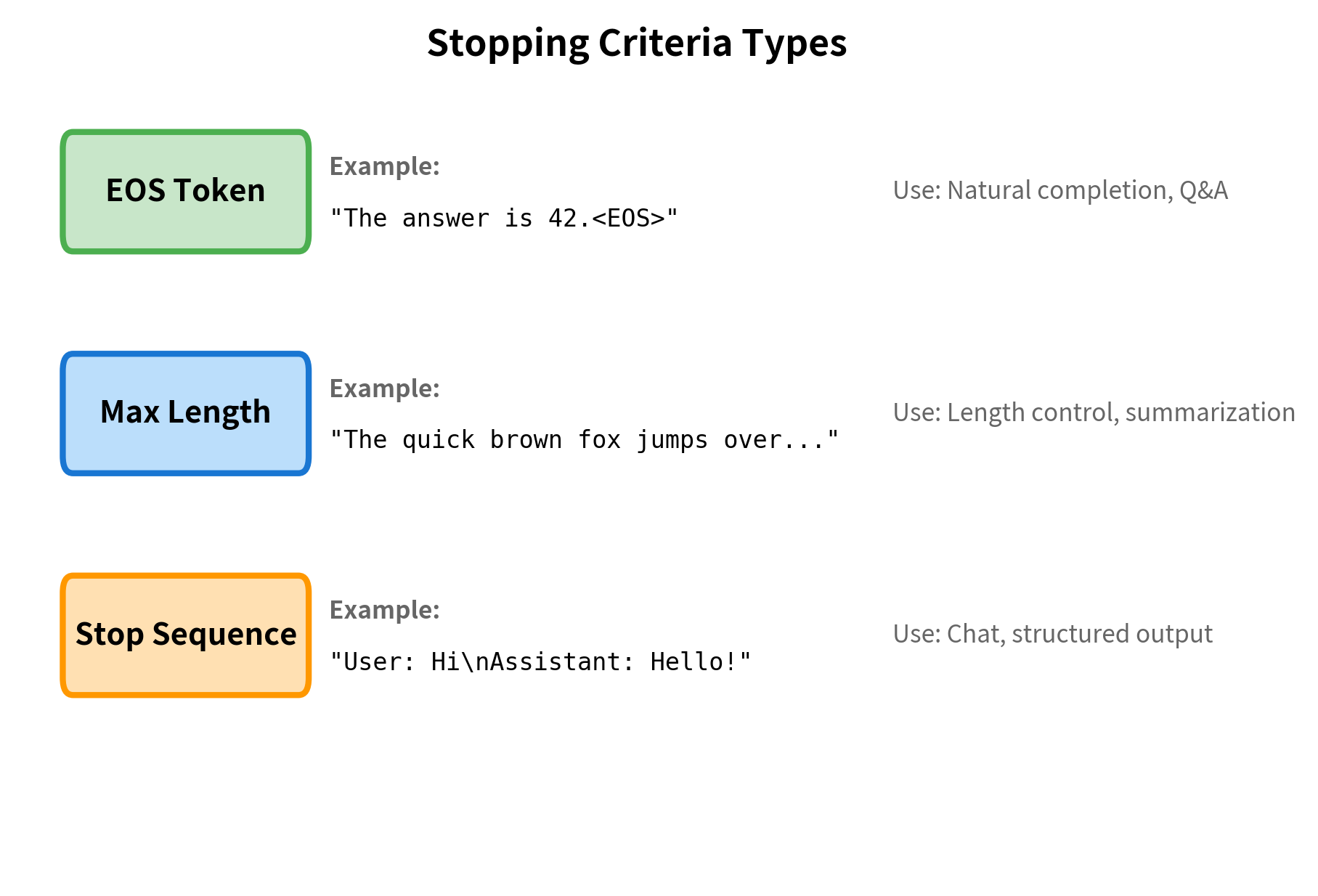
Generation must stop at some point. Without explicit stopping criteria, the model would continue generating tokens indefinitely (or until hitting a maximum length). Several strategies determine when to halt generation.

End-of-Sequence Token

The most common stopping criterion is the end-of-sequence (EOS) token. During training, sequences end with a special token that signals completion. When the model generates this token, we stop:

In[21]:
Code
def generate_until_eos(model, tokenizer, prompt, max_length=100):
    """Generate until EOS token or max length."""
    input_ids = tokenizer.encode(prompt, return_tensors="pt")

    for _ in range(max_length):
        with torch.no_grad():
            outputs = model(input_ids)
            next_token_id = outputs.logits[:, -1, :].argmax(
                dim=-1, keepdim=True
            )

        input_ids = torch.cat([input_ids, next_token_id], dim=1)

        # Stop if EOS generated
        if next_token_id.item() == tokenizer.eos_token_id:
            break

    return tokenizer.decode(input_ids[0], skip_special_tokens=True)

The EOS token works well for tasks with natural endings, like completing a sentence or answering a question. However, some prompts don't have clear endpoints, and the model may never generate EOS.

Maximum Length

A hard maximum length prevents runaway generation:

In[22]:
Code
def generate_with_max_length(model, tokenizer, prompt, max_new_tokens=50):
    """Generate exactly max_new_tokens (unless EOS encountered)."""
    input_ids = tokenizer.encode(prompt, return_tensors="pt")
    prompt_length = input_ids.size(1)
    max_total_length = prompt_length + max_new_tokens

    while input_ids.size(1) < max_total_length:
        with torch.no_grad():
            outputs = model(input_ids)
            next_token_id = outputs.logits[:, -1, :].argmax(
                dim=-1, keepdim=True
            )

        input_ids = torch.cat([input_ids, next_token_id], dim=1)

        if next_token_id.item() == tokenizer.eos_token_id:
            break

    return tokenizer.decode(input_ids[0], skip_special_tokens=True)

Stop Sequences

For specific applications, we might want to stop when certain text patterns appear. This is common in chat applications where we stop at user turn markers:

In[23]:
Code
def generate_until_stop_sequence(
    model,
    tokenizer,
    prompt: str,
    stop_sequences: list[str],
    max_new_tokens: int = 100,
):
    """Generate until a stop sequence is found in the output."""
    input_ids = tokenizer.encode(prompt, return_tensors="pt")

    for _ in range(max_new_tokens):
        with torch.no_grad():
            outputs = model(input_ids)
            next_token_id = outputs.logits[:, -1, :].argmax(
                dim=-1, keepdim=True
            )

        input_ids = torch.cat([input_ids, next_token_id], dim=1)

        # Check for stop sequences in generated text
        current_text = tokenizer.decode(input_ids[0], skip_special_tokens=True)
        for stop_seq in stop_sequences:
            if stop_seq in current_text[len(prompt) :]:
                # Truncate at stop sequence
                stop_idx = current_text.find(stop_seq, len(prompt))
                return current_text[:stop_idx]

        if next_token_id.item() == tokenizer.eos_token_id:
            break

    return tokenizer.decode(input_ids[0], skip_special_tokens=True)
Out[24]:
Console
Prompt: List three colors: 1. Red 2.
Stop sequences: ['\n\n', '4.']
Generated: List three colors: 1. Red 2. Blue 3. Yellow 

The generation stopped as soon as it encountered one of our specified patterns. This is particularly useful for structured outputs where you know the format in advance, such as generating exactly three items in a list or stopping at the end of an assistant's turn in a conversation.

Multiple Stopping Criteria

In practice, we often combine multiple criteria. The Hugging Face library supports this through StoppingCriteria objects:

In[25]:
Code
from transformers import StoppingCriteria


class MaxTokensCriteria(StoppingCriteria):
    """Stop after generating max_tokens new tokens."""

    def __init__(self, start_length: int, max_new_tokens: int):
        self.start_length = start_length
        self.max_new_tokens = max_new_tokens

    def __call__(self, input_ids, scores, **kwargs):
        return input_ids.shape[1] >= self.start_length + self.max_new_tokens


class StopStringCriteria(StoppingCriteria):
    """Stop when a specific string appears in the output."""

    def __init__(self, tokenizer, stop_string: str, start_length: int):
        self.tokenizer = tokenizer
        self.stop_string = stop_string
        self.start_length = start_length

    def __call__(self, input_ids, scores, **kwargs):
        generated_text = self.tokenizer.decode(
            input_ids[0, self.start_length :], skip_special_tokens=True
        )
        return self.stop_string in generated_text
Out[26]:
Visualization
Diagram showing three types of stopping criteria with example scenarios.
Different stopping criteria and their typical use cases. EOS tokens work for natural completions, max length prevents runaway generation, and stop sequences enable structured outputs like chat turns or list items.

Generation Speed Optimization

Beyond KV caching, several techniques can accelerate generation. These optimizations are crucial for production deployments where latency directly impacts user experience.

Batch Processing

Processing multiple prompts simultaneously amortizes the overhead of loading model weights. The attention computation is parallelized across the batch dimension:

In[27]:
Code
def batch_generate(
    model,
    tokenizer,
    prompts: list[str],
    max_new_tokens: int = 30,
):
    """Generate completions for multiple prompts in parallel."""
    # Tokenize all prompts with padding
    inputs = tokenizer(
        prompts,
        return_tensors="pt",
        padding=True,
        truncation=True,
    )

    # Generate for all prompts at once
    with torch.no_grad():
        outputs = model.generate(
            **inputs,
            max_new_tokens=max_new_tokens,
            pad_token_id=tokenizer.eos_token_id,
            do_sample=False,
        )

    # Decode all outputs
    return [
        tokenizer.decode(output, skip_special_tokens=True) for output in outputs
    ]
Out[28]:
Console
A decoder-only architecture is being used, but right-padding was detected! For correct generation results, please set `padding_side='left'` when initializing the tokenizer.
Batch generation (4 prompts): 0.525s
Sequential generation: 2.244s
Speedup: 4.3×

Batch generation processes all four prompts faster than running them one at a time. The speedup comes from amortizing the model loading overhead and parallelizing the attention computations across the batch dimension. This makes batching essential for high-throughput serving scenarios.

Mixed Precision

Using half-precision (float16) or brain floating point (bfloat16) reduces memory bandwidth and enables faster computation on modern GPUs:

In[29]:
Code
# Load model in half precision
model_fp16 = GPT2LMHeadModel.from_pretrained(
    "gpt2",
    torch_dtype=torch.float16,
    device_map="auto" if torch.cuda.is_available() else None,
)

The memory savings from half precision are substantial:

Out[30]:
Console
Model size comparison:
  Float32: 474.7 MB
  Float16: 237.4 MB (theoretical)
  Memory reduction: 50%

Cutting the model precision in half directly halves the memory footprint, allowing larger batch sizes or longer sequences to fit in the same GPU memory. On modern GPUs with tensor cores, float16 operations are also faster than float32, providing both memory and speed benefits.

Speculative Decoding

Speculative decoding uses a smaller "draft" model to propose multiple tokens, then verifies them with the larger model in a single forward pass. When predictions align, multiple tokens are accepted at once:

Out[31]:
Visualization
Diagram showing draft model proposing tokens and target model verifying them in parallel.
Speculative decoding workflow. A fast draft model proposes k tokens, which are verified by the target model in parallel. Matching tokens are accepted, mismatches trigger rejection and resampling. This can provide 2-3× speedup when draft and target models agree frequently.

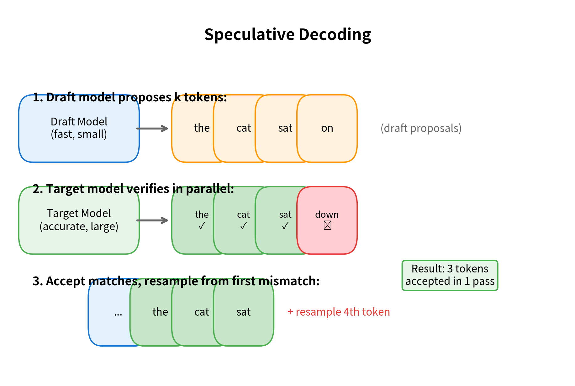
The effectiveness of speculative decoding depends on how well the draft model predicts the target model's outputs. When they agree frequently, significant speedups are possible. When they disagree often, the overhead of running two models provides little benefit.
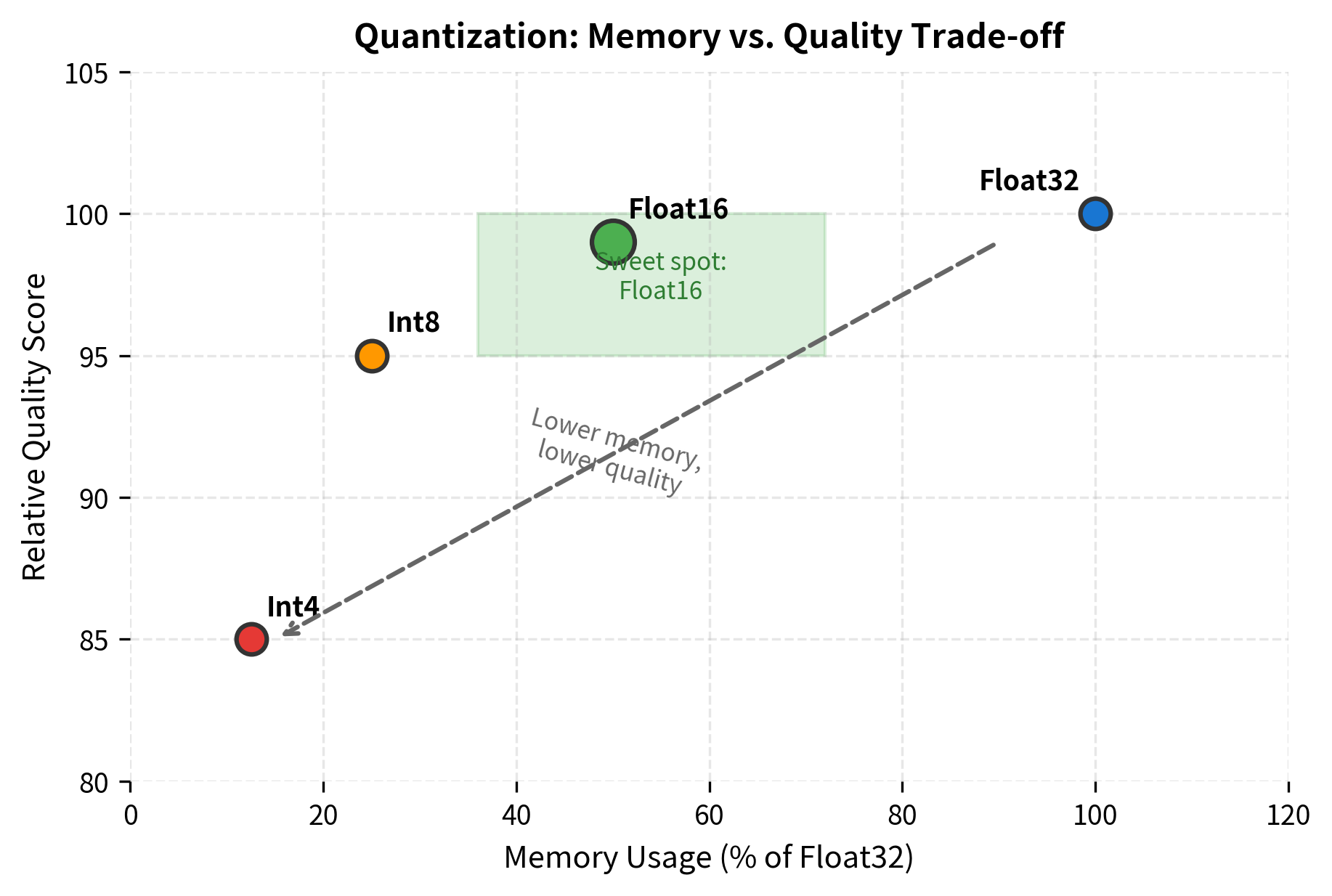
Quantization

Reducing model precision further with quantization (8-bit, 4-bit, or even lower) enables faster inference with reduced memory:

Out[32]:
Console
Quantization trade-offs:
------------------------------------------------------------
Precision    Memory       Speed        Quality        
------------------------------------------------------------
Float32      100%         1×           Baseline       
Float16      50%          ~1.5×        Minimal loss   
Int8         25%          ~2×          Small loss     
Int4         12.5%        ~3×          Noticeable loss

The trade-off between precision and quality is application-dependent. For many tasks, float16 provides virtually identical results to float32. Int8 quantization typically works well for inference with minimal degradation. Int4 can cause noticeable quality loss but enables running much larger models on limited hardware.
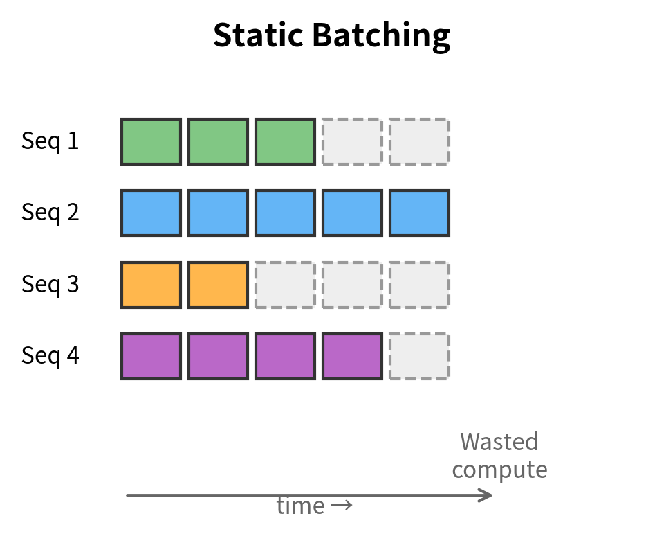
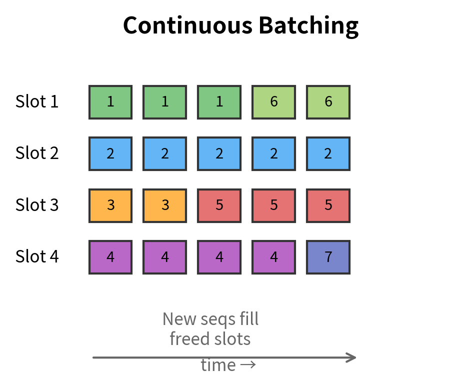
Out[33]:
Visualization
Scatter plot showing four precision levels (Float32, Float16, Int8, Int4) with memory usage on x-axis and relative quality on y-axis, with Float16 highlighted as the optimal balance point.
Quantization trade-offs between memory usage and model quality. Lower precision reduces memory requirements dramatically but may degrade output quality. Float16 is typically the sweet spot for inference, offering 50% memory reduction with minimal quality loss.

Continuous Batching

For serving multiple users, continuous batching (also called in-flight batching) dynamically adds and removes sequences from a batch as they complete. This maximizes GPU utilization compared to static batching where all sequences must wait for the longest one:

Out[34]:
Visualization
Static batching: All sequences wait for the longest one to complete. Dashed boxes show wasted compute from padding shorter sequences.
Continuous batching: New sequences fill slots as they become available. Numbers indicate different sequences being processed, with new ones (5, 6, 7) entering as earlier ones finish.

Complete Generation Implementation

Let's put everything together into a complete, production-quality generation function:

In[35]:
Code
from dataclasses import dataclass


@dataclass
class GenerationConfig:
    """Configuration for text generation."""

    max_new_tokens: int = 50
    temperature: float = 1.0
    top_k: int | None = None
    top_p: float | None = None
    repetition_penalty: float = 1.0
    stop_sequences: list[str] | None = None


def generate_with_config(
    model,
    tokenizer,
    prompt: str,
    config: GenerationConfig,
) -> str:
    """
    Complete generation function with configurable sampling strategies.

    Supports temperature scaling, top-k sampling, nucleus sampling,
    repetition penalty, and stop sequences.
    """
    input_ids = tokenizer.encode(prompt, return_tensors="pt")
    attention_mask = torch.ones_like(input_ids)
    generated_ids = input_ids.clone()
    past_key_values = None

    for _ in range(config.max_new_tokens):
        with torch.no_grad():
            if past_key_values is not None:
                current_input = generated_ids[:, -1:]
            else:
                current_input = generated_ids

            outputs = model(
                input_ids=current_input,
                attention_mask=attention_mask,
                past_key_values=past_key_values,
                use_cache=True,
            )
            past_key_values = outputs.past_key_values
            logits = outputs.logits[:, -1, :]

            # Apply repetition penalty
            if config.repetition_penalty != 1.0:
                for token_id in generated_ids[0].unique():
                    logits[0, token_id] /= config.repetition_penalty

            # Apply temperature
            if config.temperature != 1.0:
                logits = logits / config.temperature

            # Apply top-k filtering
            if config.top_k is not None:
                top_k_logits, top_k_indices = torch.topk(logits, config.top_k)
                logits = torch.full_like(logits, float("-inf"))
                logits.scatter_(1, top_k_indices, top_k_logits)

            # Apply nucleus (top-p) filtering
            if config.top_p is not None:
                sorted_logits, sorted_indices = torch.sort(
                    logits, descending=True
                )
                cumulative_probs = torch.cumsum(
                    F.softmax(sorted_logits, dim=-1), dim=-1
                )
                sorted_indices_to_remove = cumulative_probs > config.top_p
                sorted_indices_to_remove[:, 1:] = sorted_indices_to_remove[
                    :, :-1
                ].clone()
                sorted_indices_to_remove[:, 0] = False
                indices_to_remove = sorted_indices_to_remove.scatter(
                    1, sorted_indices, sorted_indices_to_remove
                )
                logits[indices_to_remove] = float("-inf")

            # Sample from distribution
            probs = F.softmax(logits, dim=-1)
            next_token = torch.multinomial(probs, num_samples=1)

            generated_ids = torch.cat([generated_ids, next_token], dim=1)
            attention_mask = torch.cat(
                [
                    attention_mask,
                    torch.ones((1, 1), dtype=attention_mask.dtype),
                ],
                dim=1,
            )

            # Check EOS
            if next_token.item() == tokenizer.eos_token_id:
                break

            # Check stop sequences
            if config.stop_sequences:
                current_text = tokenizer.decode(
                    generated_ids[0], skip_special_tokens=True
                )
                for stop_seq in config.stop_sequences:
                    if stop_seq in current_text[len(prompt) :]:
                        idx = current_text.find(stop_seq, len(prompt))
                        return current_text[:idx]

    return tokenizer.decode(generated_ids[0], skip_special_tokens=True)
Out[36]:
Console
Prompt: The meaning of life is

----------------------------------------------------------------------
Greedy (temp=0.01)  : not the same as the meaning of death.

The meaning of life i...
Creative (temp=1.2) : overrated nonsense.

There is a battle of words in the very ...
Top-k=50            : so narrow, and even in what the senses of the dead are able ...
Nucleus p=0.9       : profound. It is to know the worthiness of the life to which ...

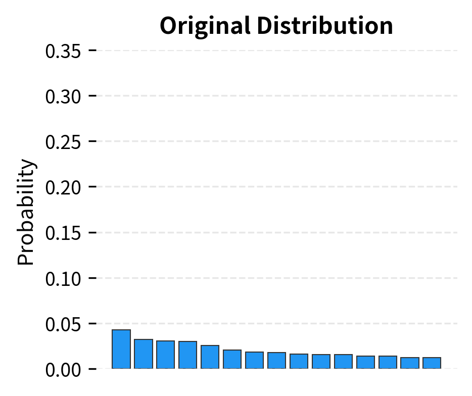
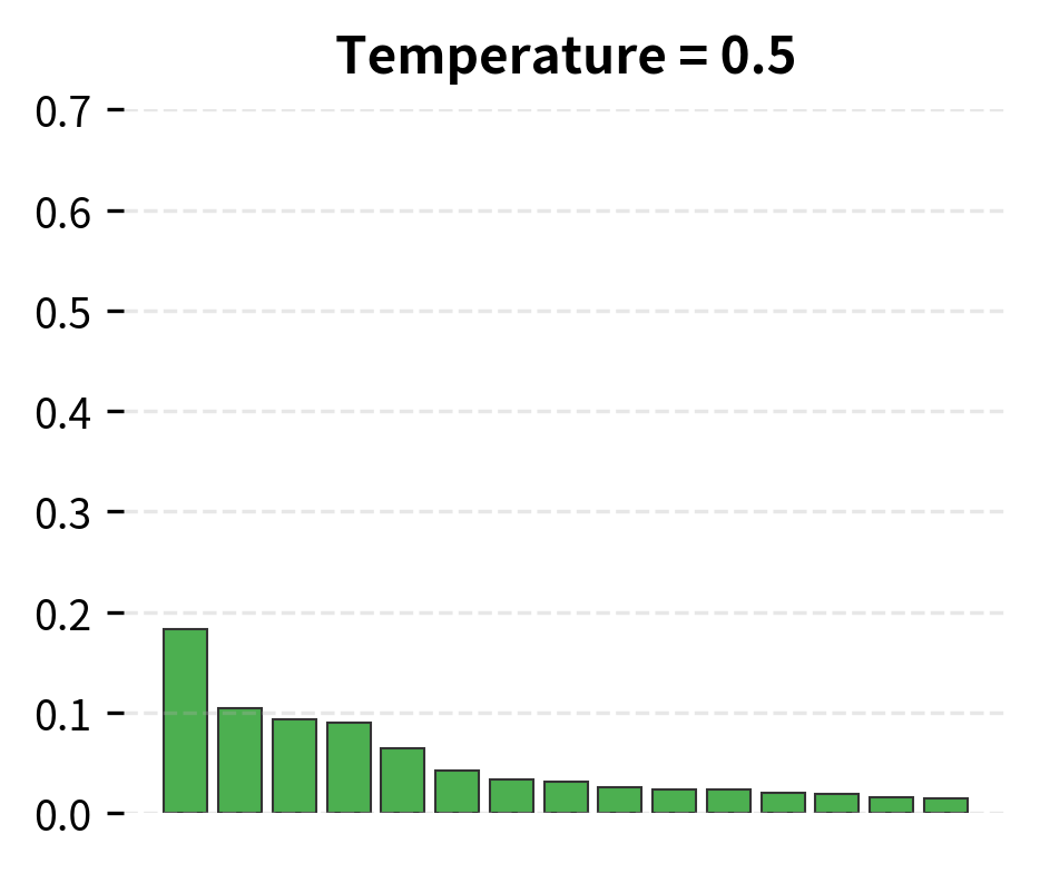
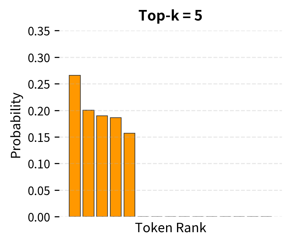
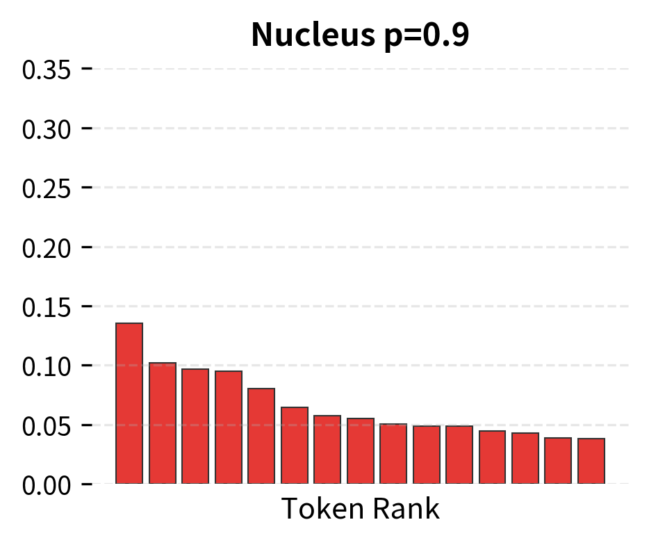
The different configurations produce noticeably different outputs. Near-greedy decoding (low temperature) gives focused, predictable completions. Higher temperature introduces more variety but can become less coherent. Top-k and nucleus sampling offer different ways to balance diversity and quality. The right choice depends on your application: creative writing benefits from higher diversity, while factual Q&A typically works better with lower temperature.

Out[37]:
Visualization
Original probability distribution from the model. Most probability mass concentrates in the top tokens, with a long tail of low-probability options.
Temperature = 0.5 sharpens the distribution, making the top token even more dominant. Lower temperature reduces randomness.
Top-k = 5 truncates to only the 5 most likely tokens (orange), zeroing out the rest (gray). Remaining probabilities are renormalized.
Nucleus (top-p = 0.9) keeps the smallest set of tokens whose cumulative probability exceeds 90% (red). This adapts to the distribution shape.

Limitations and Considerations

Autoregressive generation, while powerful, comes with inherent limitations that affect both capability and deployment.

The sequential nature of generation creates a fundamental latency floor. No matter how fast each token can be generated, producing 100 tokens requires at least 100 sequential steps. This contrasts with encoding, where an entire sequence can be processed in parallel. For applications requiring very long outputs, this sequential bottleneck becomes significant. Techniques like speculative decoding and parallel draft trees attempt to mitigate this, but the fundamental constraint remains.

KV cache memory grows linearly with sequence length, which can become problematic for very long contexts. A 7B parameter model with 32 layers and a 128K context window might require tens of gigabytes just for the cache. This has motivated research into cache compression techniques like sliding window attention, sparse attention patterns, and cache eviction strategies. Some systems maintain only a fixed-size cache of the most recent tokens, trading off the ability to attend to distant context for bounded memory usage.

The quality of generated text depends heavily on decoding strategy. Greedy decoding, while deterministic, often produces repetitive or generic outputs. Temperature sampling introduces diversity but can also produce incoherent text at high temperatures. Beam search explores multiple hypotheses but tends toward generic, high-probability sequences. Finding the right balance for each application requires experimentation.

Summary

Autoregressive generation is the fundamental process by which decoder-only transformers produce text. The key concepts covered in this chapter include:

  • Generation loop: At each step, the model predicts a probability distribution over the vocabulary, samples or selects the next token, appends it to the sequence, and repeats until a stopping criterion is met.

  • KV caching: By caching the key and value projections from previous positions, we avoid redundant computation during generation. This transforms the computational cost from quadratic to linear in sequence length, making practical generation possible.

  • Stopping criteria: Generation can terminate via EOS tokens for natural endings, maximum length limits for bounded outputs, or custom stop sequences for structured outputs like chat turns.

  • Speed optimizations: Batch processing, mixed precision, speculative decoding, quantization, and continuous batching all contribute to making generation practical for production deployments.

  • Memory trade-offs: KV caching trades memory for computation. For long sequences or large batch sizes, cache memory can become a significant constraint.

The generation procedure we've explored here forms the foundation for all the decoding strategies covered in subsequent chapters. Temperature scaling, top-k sampling, nucleus sampling, and repetition penalties all operate within this basic framework, modifying how we select the next token from the model's predicted distribution.

Key Parameters

When implementing autoregressive generation, these parameters have the most significant impact on behavior and performance:

  • max_new_tokens: Maximum number of tokens to generate. Set based on your application's typical output length. Shorter limits reduce latency and memory usage. Longer limits allow more complete responses but increase the risk of degenerate outputs.

  • temperature: Controls the randomness of token selection (covered in detail in the next chapter). Values below 1.0 make the distribution sharper, favoring high-probability tokens. Values above 1.0 flatten the distribution, increasing diversity. Use 0.0-0.3 for factual tasks, 0.7-1.0 for creative tasks.

  • use_cache: Whether to use KV caching for efficient generation. Should almost always be True for inference. Only disable for debugging or when memory is extremely constrained.

  • pad_token_id: Token ID used for padding in batched generation. Must be set to a valid token ID (often the EOS token ID) to avoid errors with variable-length sequences.

  • do_sample: Whether to sample from the probability distribution (True) or use greedy decoding (False). Greedy decoding is deterministic but often repetitive. Sampling introduces variety but requires tuning temperature and other sampling parameters.

  • stop_sequences: List of strings that trigger generation to stop. Useful for structured outputs, chat applications, and preventing runaway generation. Processed after each token, so slight performance overhead.

  • batch_size: Number of sequences to generate in parallel. Larger batches improve throughput but increase memory usage. Find the sweet spot based on your GPU memory and latency requirements.

Quiz

Ready to test your understanding? Take this quick quiz to reinforce what you've learned about autoregressive generation and KV caching.

Loading component...
Track your reading progress

Sign in to mark chapters as read and track your learning journey

Sign in →

Comments

Reference

BIBTEXAcademic
@misc{autoregressivegenerationhowgptgeneratestexttokenbytoken, author = {Michael Brenndoerfer}, title = {Autoregressive Generation: How GPT Generates Text Token by Token}, year = {2025}, url = {https://mbrenndoerfer.com/writing/autoregressive-generation-gpt-text-generation}, organization = {mbrenndoerfer.com}, note = {Accessed: 2025-12-19} }
APAAcademic
Michael Brenndoerfer (2025). Autoregressive Generation: How GPT Generates Text Token by Token. Retrieved from https://mbrenndoerfer.com/writing/autoregressive-generation-gpt-text-generation
MLAAcademic
Michael Brenndoerfer. "Autoregressive Generation: How GPT Generates Text Token by Token." 2025. Web. 12/19/2025. <https://mbrenndoerfer.com/writing/autoregressive-generation-gpt-text-generation>.
CHICAGOAcademic
Michael Brenndoerfer. "Autoregressive Generation: How GPT Generates Text Token by Token." Accessed 12/19/2025. https://mbrenndoerfer.com/writing/autoregressive-generation-gpt-text-generation.
HARVARDAcademic
Michael Brenndoerfer (2025) 'Autoregressive Generation: How GPT Generates Text Token by Token'. Available at: https://mbrenndoerfer.com/writing/autoregressive-generation-gpt-text-generation (Accessed: 12/19/2025).
SimpleBasic
Michael Brenndoerfer (2025). Autoregressive Generation: How GPT Generates Text Token by Token. https://mbrenndoerfer.com/writing/autoregressive-generation-gpt-text-generation
Michael Brenndoerfer

About the author: Michael Brenndoerfer

All opinions expressed here are my own and do not reflect the views of my employer.

Michael currently works as an Associate Director of Data Science at EQT Partners in Singapore, leading AI and data initiatives across private capital investments.

With over a decade of experience spanning private equity, management consulting, and software engineering, he specializes in building and scaling analytics capabilities from the ground up. He has published research in leading AI conferences and holds expertise in machine learning, natural language processing, and value creation through data.

Stay updated

Get notified when I publish new articles on data and AI, private equity, technology, and more.

No spam, unsubscribe anytime.

or

Create a free account to unlock exclusive features, track your progress, and join the conversation.

No popupsUnobstructed readingCommenting100% Free