

Master DeBERTa's disentangled attention mechanism that separates content and position representations. Understand relative position encoding, Enhanced Mask Decoder, and DeBERTa-v3's ELECTRA-style training that achieved state-of-the-art NLU performance.

This article is part of the free-to-read Language AI Handbook
Choose your expertise level to adjust how many terms are explained. Beginners see more tooltips, experts see fewer to maintain reading flow. Hover over underlined terms for instant definitions.
DeBERTa
BERT's attention mechanism treats content and position as inseparable. When a token attends to another, its query vector combines both what the token means and where it sits in the sequence. This entanglement seems natural, but it limits how flexibly the model can reason about content and position independently. What if we could disentangle these two signals?
DeBERTa (Decoding-enhanced BERT with Disentangled Attention) introduced exactly this separation. Published by Microsoft Research in 2020, DeBERTa maintains separate representations for content and position, then computes attention using three distinct components: content-to-content, content-to-position, and position-to-content. This disentangled formulation gives the model finer control over how tokens relate to each other.
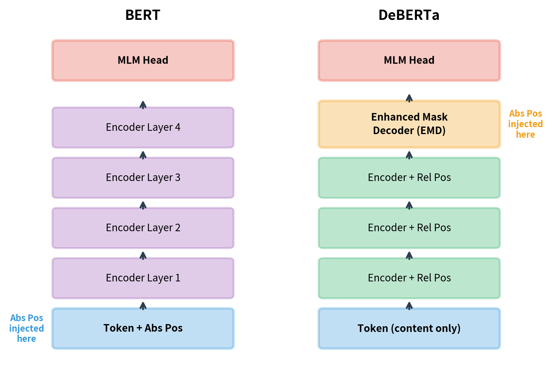
The architecture also rethinks when position information enters the model. BERT adds absolute position embeddings at the input layer, before any transformer processing. DeBERTa delays absolute position injection until just before the output layer, using relative positions throughout the encoder. This seemingly small change has profound effects on how the model learns positional patterns.
In this chapter, we'll dissect DeBERTa's attention mechanism, understand why disentanglement helps, implement the core components, and examine the improvements that led to DeBERTa-v3.
The Problem with Entangled Attention
Standard BERT attention combines content and position by adding position embeddings to token embeddings at the input layer:
where:
- : the initial hidden representation for a token before any transformer layers
- : the token embedding looked up from the vocabulary embedding table
- : the position embedding encoding the token's absolute position in the sequence
From this point forward, every hidden state is a mixture of content and position information. When computing attention scores, the query and key vectors both contain this entangled representation:
where:
- : the attention score between query position and key position
- : the query vector at position , computed from the entangled hidden state
- : the key vector at position , computed from the entangled hidden state
- : the dimension of the query and key vectors (used for scaling)
- : the dot product measuring similarity between query and key
Since and each encode both the content at positions and and the absolute positions themselves, the model cannot separately ask "what content is at position ?" and "what is the relative position of to ?" These questions are conflated in a single dot product.
In entangled attention (BERT), content and position are combined before attention, so the model cannot reason about them independently. In disentangled attention (DeBERTa), content and position maintain separate representations, allowing the model to compute distinct attention scores for content-content relationships and position-position relationships.
Consider the sentence "The cat sat on the mat." When determining how "sat" should attend to "cat," two factors matter:
- Content relationship: "sat" is a verb that often takes animate subjects like "cat"
- Positional relationship: "cat" appears two positions before "sat," which is a typical subject-verb distance
BERT's entangled attention computes a single score that mixes these signals. DeBERTa computes them separately and combines them, giving each factor explicit representation in the attention computation.
Both approaches produce representations of the same shape, but the DeBERTa style maintains two separate tensors. This separation allows the attention mechanism to explicitly model how content relates to content versus how content relates to position, rather than conflating these two signals.
Disentangled Attention Formulation
Now that we understand why entangled representations limit the model's expressiveness, let's develop the mathematical framework for disentangled attention. The key insight is deceptively simple: instead of computing one attention score that mixes content and position, we compute separate scores for each type of relationship and combine them.
Building Intuition: What Questions Should Attention Answer?
When token decides how much to attend to token , it implicitly asks several questions:
-
"Is the meaning at position relevant to my meaning?" This is a pure semantic question. The word "bank" should attend strongly to "river" or "money" based on meaning alone, regardless of where these words appear in the sentence.
-
"Given what I mean, is the relative position of important?" Certain words care about specific positional relationships. A verb might strongly attend to whatever appears 1-2 positions before it (likely the subject), regardless of what word occupies that position.
-
"Given my position relative to , is the content at important?" Position can make content more or less relevant. The first token in a sentence might particularly care about proper nouns, while a token near the end might care more about punctuation.
Standard attention conflates all three questions into a single dot product. Disentangled attention answers each explicitly.
The Disentangled Attention Formula
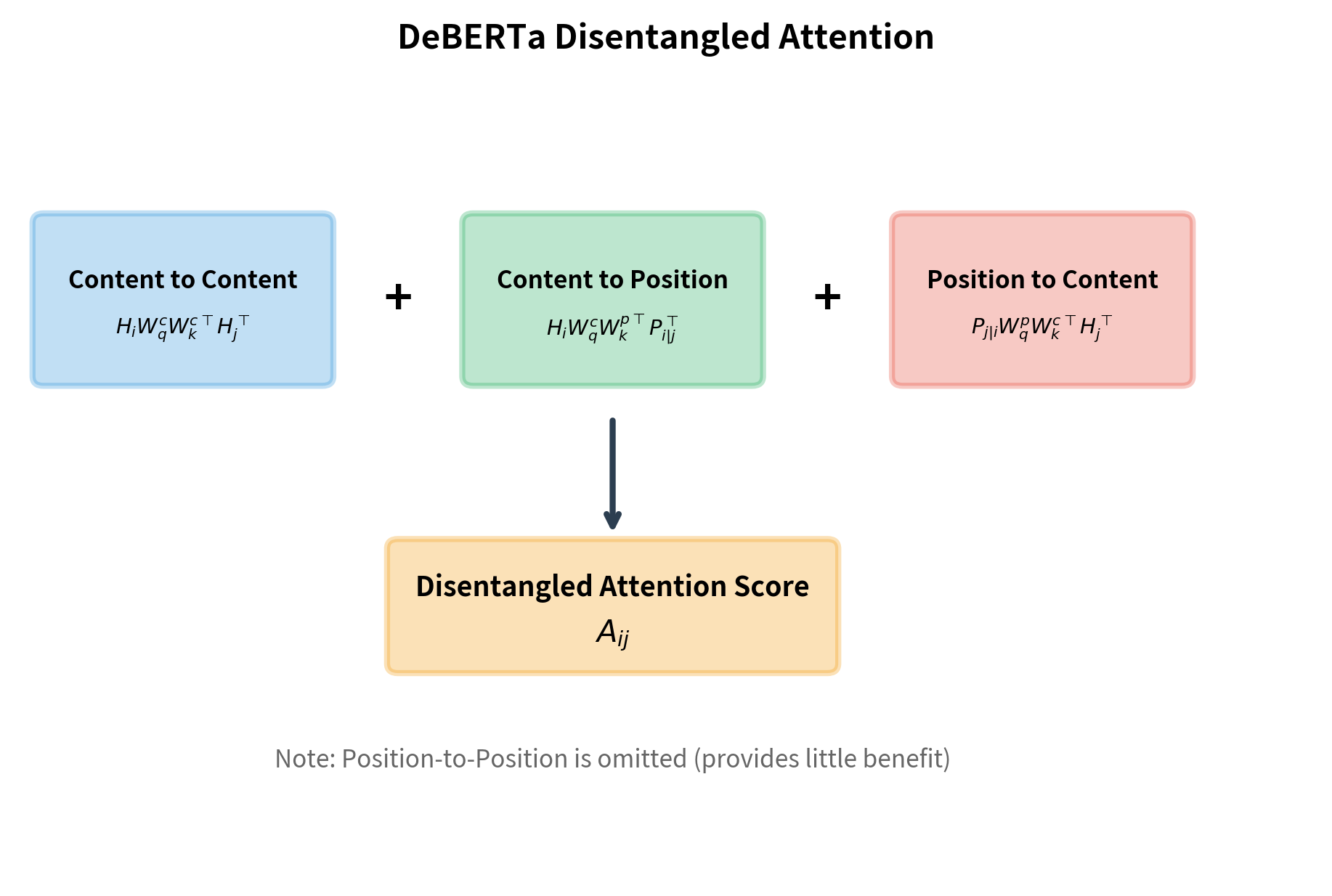
With this intuition, we can write the attention score as a sum of three terms:
Let's unpack each symbol and understand why it appears where it does:
Core representations:
- , : Content vectors at positions and . These encode what the tokens mean, with no position information mixed in.
- : The relative position embedding from 's perspective looking at . If is 3 positions ahead, this encodes "+3".
- : The relative position embedding from 's perspective looking at . For the same pair, this encodes "-3".
Projection matrices:
- , : Project content vectors into query and key spaces for semantic comparison.
- , : Project position embeddings into query and key spaces for positional comparison.
The superscripts (content) and (position) distinguish which representation type each matrix operates on.
Understanding Each Term
Let's trace through what each component computes:
Term 1: Content-to-Content
This measures semantic similarity between tokens and . The content at position is projected into query space (), and the content at position is projected into key space (). Their dot product reveals how semantically related the two tokens are, completely independent of where they appear.
Term 2: Content-to-Position
Here, the content at attends to the relative position of . Notice that is projected with the content query matrix (), while the position embedding is projected with the position key matrix (). This allows the model to learn patterns like "verbs attend strongly to position -2" (where subjects typically appear).
Term 3: Position-to-Content
This flips the relationship: the relative position from 's perspective attends to the content at . This enables patterns like "the position 2 tokens before me cares about noun content." The position embedding becomes the query, and content becomes the key.
Why No Position-to-Position Term?
You might wonder: why not include a fourth term, , for position-to-position attention?
The DeBERTa authors experimented with this and found it provides negligible benefit. Intuitively, relative positions are already informative on their own. Knowing that two positions are 3 apart doesn't become more useful by also considering that 3 apart "attends to" being 3 apart. The information is redundant, and the added computation isn't worthwhile.
Visualizing Attention Component Contributions
To build intuition for how the three components interact, let's examine their typical magnitudes and how they combine:
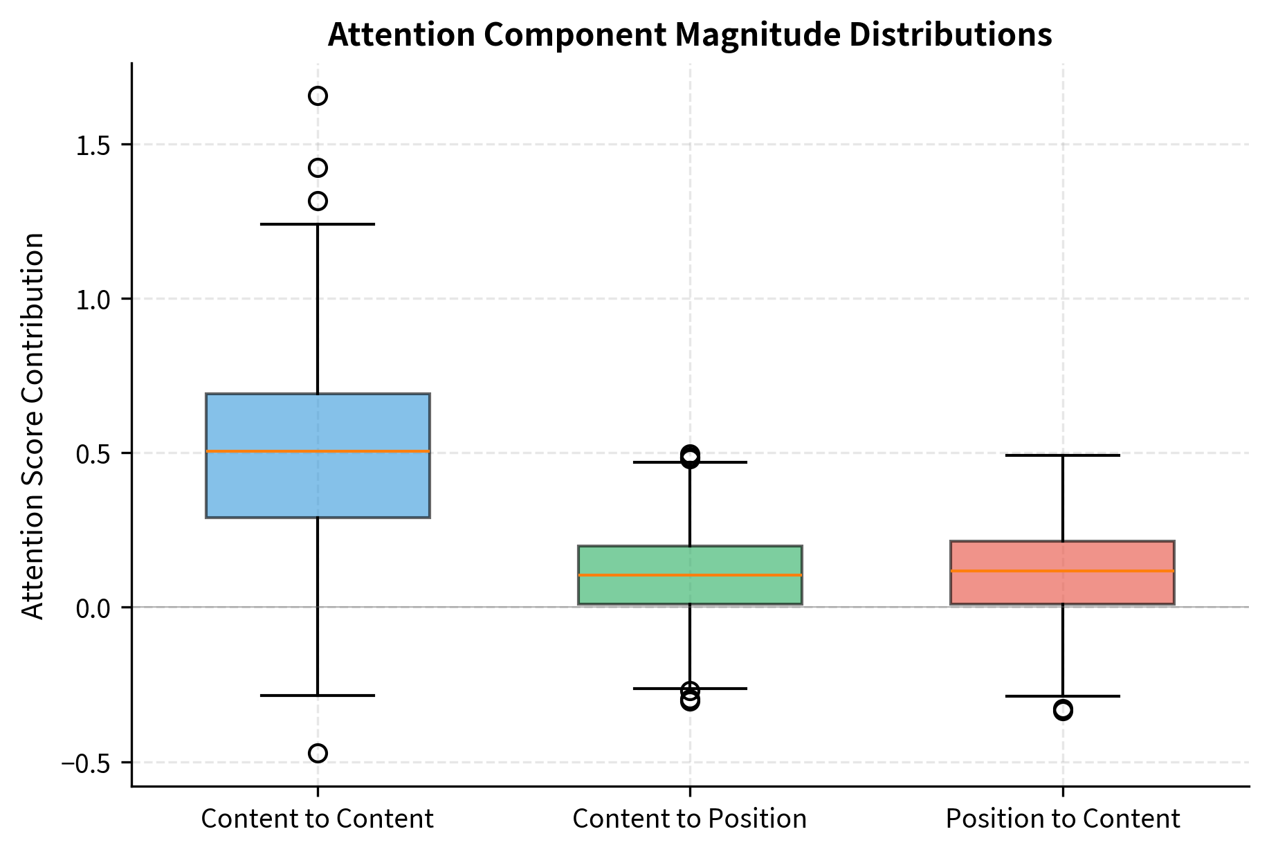
The content-to-content component typically dominates, providing the primary semantic signal. The position-related components add smaller adjustments that fine-tune attention based on relative location. This asymmetry makes sense: what tokens mean usually matters more than where they are, but position provides important context for syntactic patterns.
Relative Position Encoding
The disentangled attention formula references position embeddings and , but we haven't yet explained what these embeddings encode or how they're computed. This section develops the relative position encoding scheme that makes disentangled attention possible.
From Absolute to Relative Positions
BERT uses absolute position embeddings: position 0 gets one learned vector, position 1 gets another, and so on. Each position in the sequence has a fixed identity. While simple, this approach has a fundamental limitation: the model must learn separately that "position 2 attending to position 5" and "position 7 attending to position 10" both represent "3 tokens ahead."
Relative position encoding captures the insight that what matters is the distance between tokens, not their absolute locations. Instead of encoding "I am at position 5," a token encodes "token is 3 positions ahead of me." This single representation applies whether the token pair sits at the start, middle, or end of the sequence.
The benefits are substantial:
- Generalization: Patterns learned at one position transfer automatically to others
- Length flexibility: The model can handle sequences longer than those seen during training (to some extent)
- Linguistic alignment: Grammar often depends on relative word order, not absolute position
The Relative Position Formula
Given query position and key position , the relative position embedding encodes the distance . But we face a practical constraint: we can't have infinitely many embeddings for every possible distance. DeBERTa bounds relative positions to a maximum distance (typically 512), mapping all distances to a finite set of embeddings.
The mapping function converts a raw relative distance to an embedding index:
Let's understand each component:
- : The embedding table index we'll use to look up the position embedding
- : The raw relative distance. Negative means is ahead of ; positive means is behind
- : The maximum relative distance we encode distinctly
The three cases implement a "clip-and-shift" strategy:
-
Far ahead (): When the key is more than positions ahead, we can't distinguish exactly how far. All such positions share index 0.
-
Far behind (): Similarly, when the key is more than positions behind, all such positions share the maximum index .
-
Within range: For distances between and , we shift by to convert negative distances to non-negative indices. A distance of maps to index 0, distance 0 maps to index , and distance maps to index .
Why 2k Embeddings?
The total number of embeddings is because we need to represent distances from to :
- Negative distances ( to ): distinct values
- Zero and positive distances ( to ): distinct values
- Total: embeddings
For , this gives 1024 position embeddings, which is quite manageable memory-wise while covering the vast majority of practical attention distances.
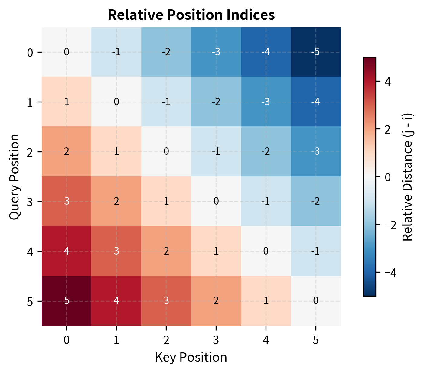
The output shape (6, 6, 64) provides a unique embedding for each query-key position pair. The relative position matrix shows the raw distances before they are clipped and shifted to valid embedding indices.
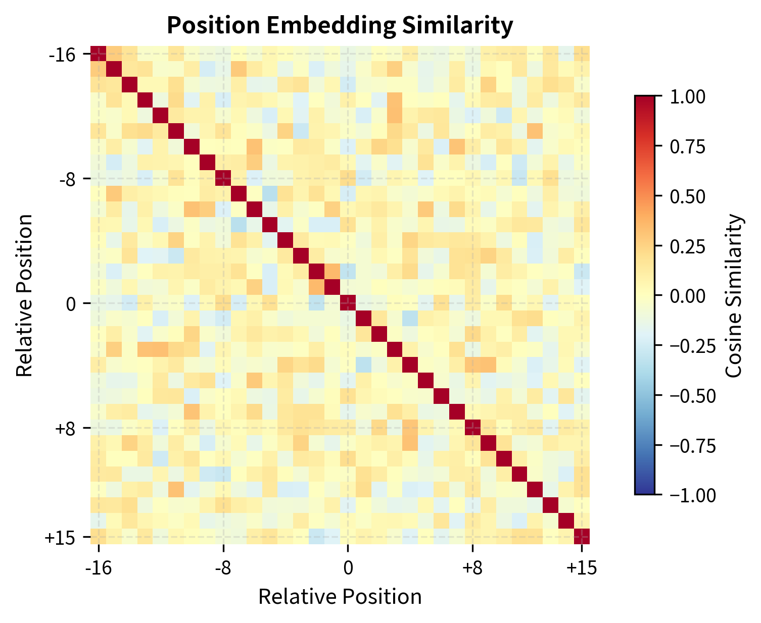
The similarity matrix reveals that nearby relative positions (e.g., +2 and +3) have more similar embeddings than distant ones (e.g., +2 and +15). This structure emerges from the learned embeddings and helps the model treat similar positional relationships similarly.
The relative position matrix shows that position 0 sees position 3 as "+3" (three positions ahead), while position 3 sees position 0 as "-3" (three positions behind). This asymmetry is captured in the embeddings and used differently in the content-to-position versus position-to-content attention terms.
Implementing Disentangled Attention
Now that we understand the mathematics, let's translate the formulas into working code. The implementation is more complex than standard attention because we must:
- Maintain separate projections for content and position
- Compute the relative position embedding matrix
- Calculate three attention components instead of one
- Combine them before applying softmax
The key insight is that each term in the attention formula corresponds to a distinct matrix multiplication in the code. Let's trace through how the formula maps to implementation.
The attention probabilities sum to 1.0 as expected, confirming that the softmax normalization works correctly across the combined attention scores. The output maintains the same shape as the input, allowing the layer to be stacked in a standard transformer architecture.
Mapping Code to Formula
Let's trace how the implementation connects to our mathematical formulation:
| Formula Term | Code Variable | Computation |
|---|---|---|
q_c | self.query_content(hidden_states) | |
k_c | self.key_content(hidden_states) | |
k_p | self.key_position(rel_pos_emb) | |
q_p | self.query_position(rel_pos_emb) | |
| Content-to-Content | attn_c2c | torch.matmul(q_c, k_c.transpose(-2, -1)) |
| Content-to-Position | attn_c2p | torch.einsum("bhid,hijd->bhij", q_c, k_p_transposed) |
| Position-to-Content | attn_p2c | torch.einsum("hjid,bhkd->bhij", q_p_transposed, k_c) |
The einsum operations handle the complex tensor contractions needed when position embeddings have different shapes than content representations. Standard matrix multiplication (torch.matmul) works for content-to-content since both tensors have the same structure.
The implementation shows how disentangled attention requires significantly more computation than standard attention. We compute three separate attention score matrices and combine them. However, the additional expressiveness often outweighs this cost for challenging NLU tasks.
Comparing Attention Patterns
Let's visualize how disentangled attention differs from standard attention by examining the three components separately:
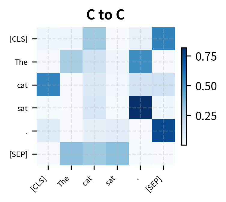
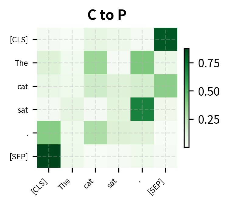
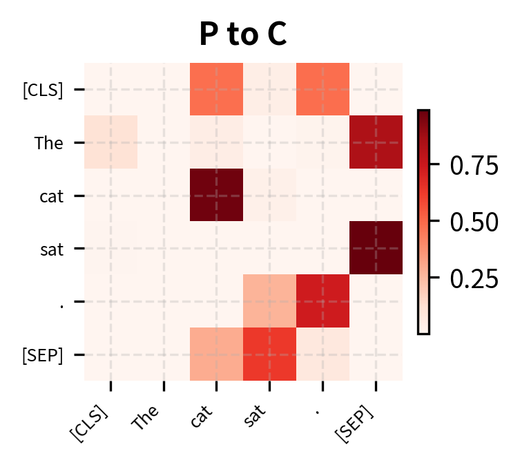
Each component captures different information. Content-to-content attention finds semantic relationships regardless of position. Content-to-position attention allows tokens to attend based on relative distance, useful for syntax patterns like subject-verb agreement. Position-to-content attention enables positional context to influence what content is attended to, helping the model learn position-dependent semantics.
Enhanced Mask Decoder
DeBERTa's second major innovation is the Enhanced Mask Decoder (EMD). BERT adds absolute position embeddings at the input layer, before any transformer processing. DeBERTa delays absolute position injection until just before the output layer.
Why does this matter? During masked language modeling, the model must predict a masked token. The prediction should depend on:
- The content of surrounding tokens (semantic context)
- The relative positions of surrounding tokens (syntactic patterns)
- The absolute position of the masked token itself (where in the sentence the prediction occurs)
By separating absolute positions from the encoder, DeBERTa can use relative positions throughout encoding, then inject absolute positions only where they matter most: at the decoding step.
The Enhanced Mask Decoder is essentially one or two additional transformer layers that incorporate absolute position information. This design has two benefits:
- Cleaner encoding: The encoder uses only relative positions, avoiding the mixing of absolute and relative signals
- Better MLM: Absolute positions are available exactly where they're needed for prediction
The EMD maintains the same tensor shape as the encoder output, allowing it to serve as a drop-in enhancement before the MLM prediction head. The two additional transformer layers with absolute position information help the model make position-aware predictions.
Complete DeBERTa Model
Let's assemble the components into a complete DeBERTa model:
The complete encoder processes token IDs through disentangled attention layers and the Enhanced Mask Decoder, producing contextualized representations. This small test model has about 230K parameters. A full DeBERTa-Base would have approximately 140M parameters, reflecting the additional position projection matrices and EMD layers compared to BERT.
DeBERTa Improvements: XLNet Integration
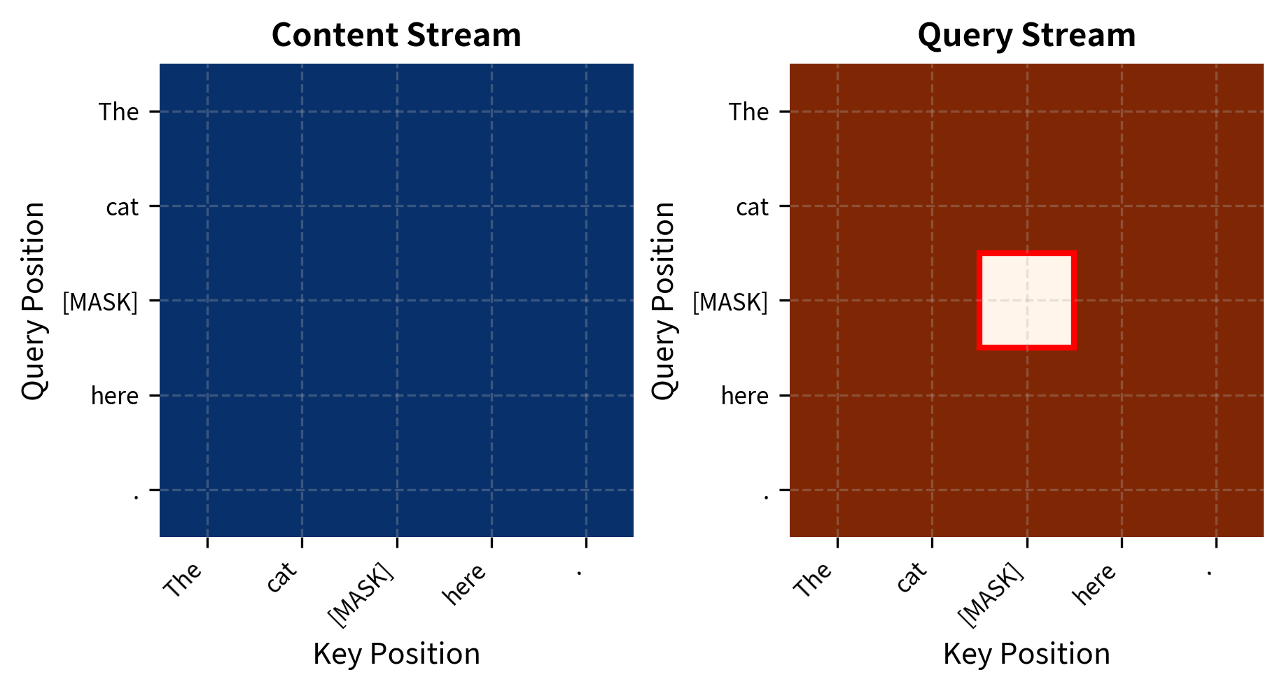
DeBERTa also incorporates ideas from XLNet, another post-BERT model. Specifically, it uses a variant of XLNet's two-stream attention during pretraining, which separates content and query representations for masked token prediction.
The key insight: when predicting a masked token, the model should not see the token's own content (that would leak the answer), but it should know the token's position (to understand positional context). Two-stream attention achieves this separation:
- Content stream: Sees all tokens including the current position
- Query stream: Sees all tokens except the current position's content
DeBERTa-v2 and v3 Advances
The original DeBERTa was followed by DeBERTa-v2 and DeBERTa-v3, each introducing further improvements.
DeBERTa-v2
DeBERTa-v2 focused on scaling and efficiency:
- Larger vocabulary: Expanded from 30K to 128K tokens using a SentencePiece tokenizer, reducing the out-of-vocabulary rate
- nGiE: Added a convolutional layer after token embeddings to capture local n-gram features
- Larger scale: Trained models up to 1.5B parameters
The nGiE layer preserves tensor shape while enriching each token's representation with local context from its neighbors. With a kernel size of 3, each output position incorporates information from the token itself plus one neighbor on each side, effectively capturing trigram patterns before the token representations enter the transformer layers.
DeBERTa-v3
DeBERTa-v3 introduced a fundamentally different pretraining approach:
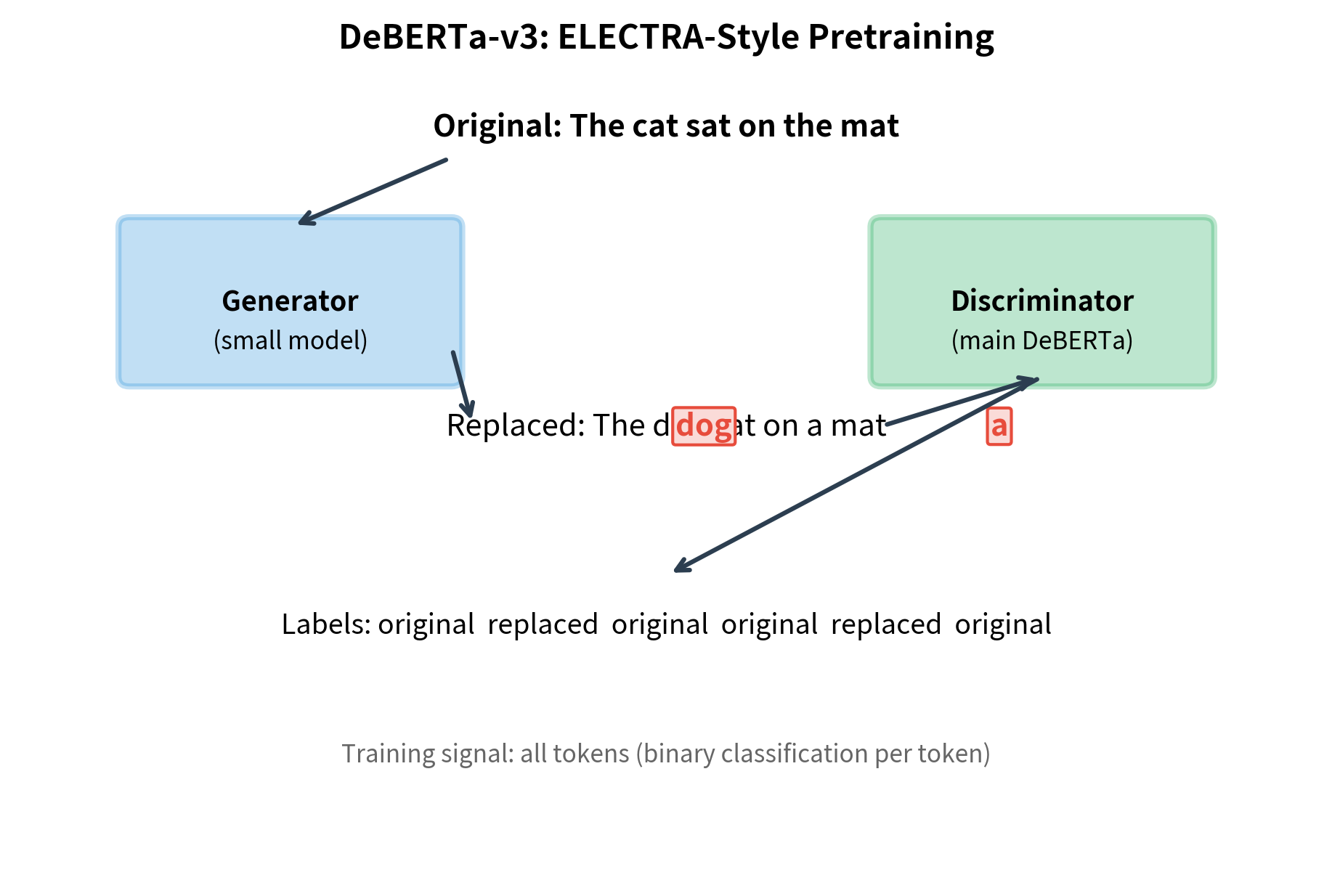
- ELECTRA-style training: Instead of masked language modeling, DeBERTa-v3 uses replaced token detection (RTD) with a generator-discriminator setup
- Gradient-disentangled embedding sharing: The generator and discriminator share embeddings, but gradients from the discriminator don't flow to the shared embeddings through the generator
- Better efficiency: RTD trains on all tokens rather than just 15% masked tokens, making pretraining more efficient
An alternative to MLM where a small generator network replaces some tokens with plausible alternatives, and the main model learns to detect which tokens were replaced. This trains on 100% of tokens (distinguishing original vs replaced) rather than 15% (predicting masked tokens).
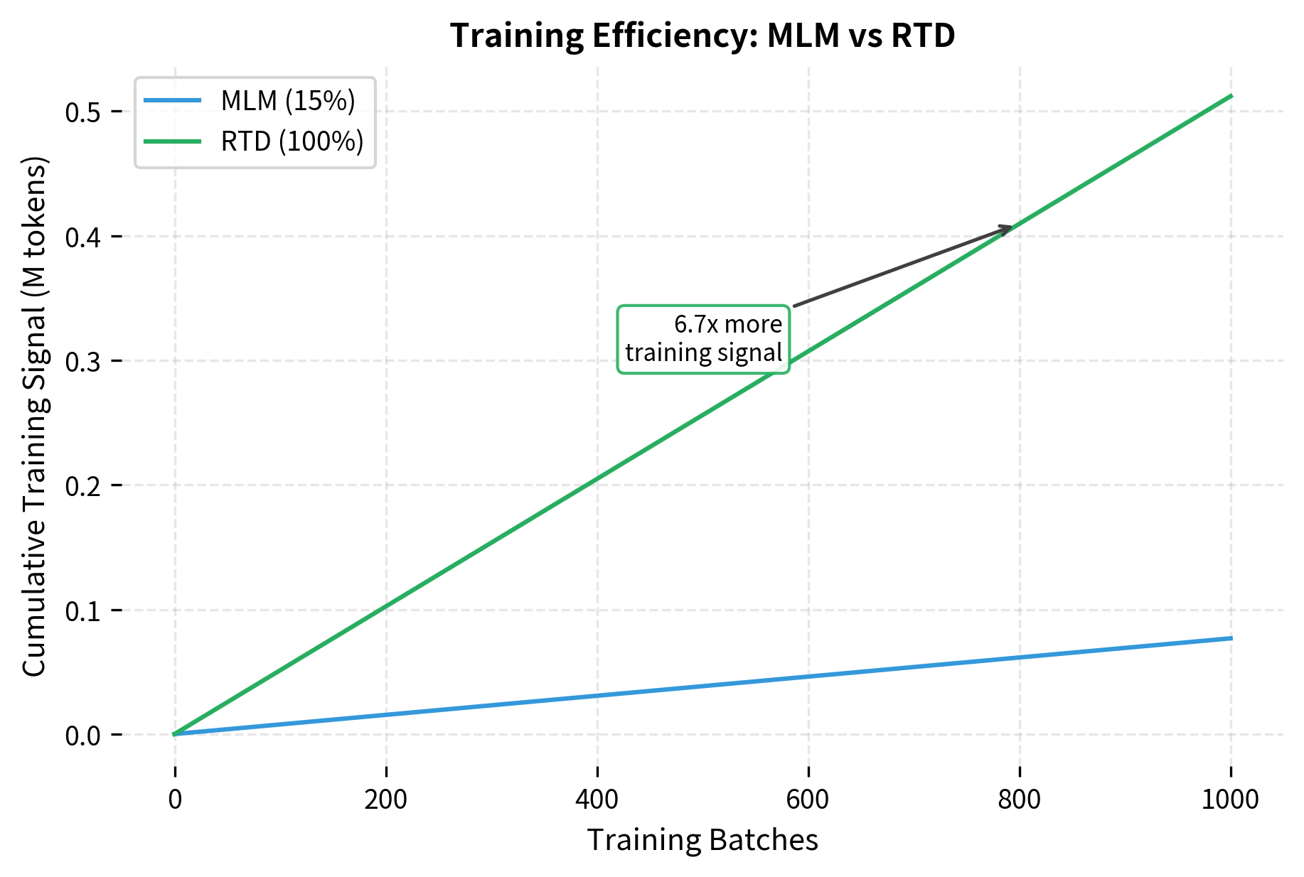
This efficiency difference is dramatic. After 1000 batches, RTD has provided training signal from approximately 512 million token positions, while MLM has only trained on about 77 million (15% of that). The 6.7x efficiency multiplier means DeBERTa-v3 can match BERT's training with far fewer compute resources, or achieve better results with the same resources.
Using Pretrained DeBERTa
In practice, you'll use DeBERTa through the Hugging Face transformers library:
The tokenizer converts the input sentence into subword tokens. Notice that [MASK] is preserved as a special token that the model will predict. The surrounding context provides the clues the model needs to fill in the blank.
The model assigns the highest logit score to "Paris" with a substantial margin over alternative predictions. The second-highest predictions might include other city names or related terms, but the correct answer dominates. This demonstrates the model's strong grasp of factual knowledge and contextual understanding.
DeBERTa correctly predicts "Paris" with high confidence. The model's disentangled attention and enhanced positional encoding help it understand that the masked position should contain a proper noun that is the capital of France.
Performance Comparison
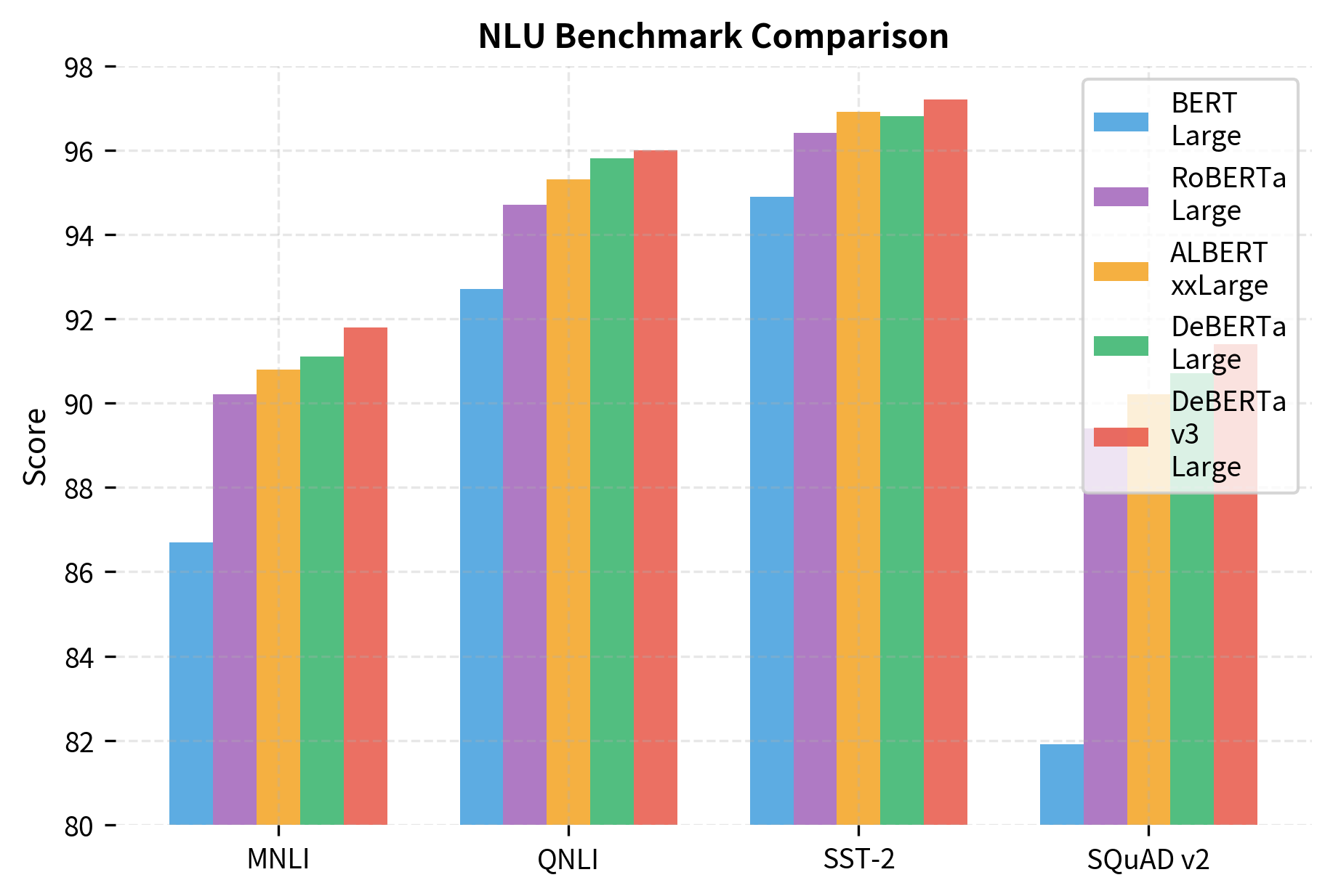
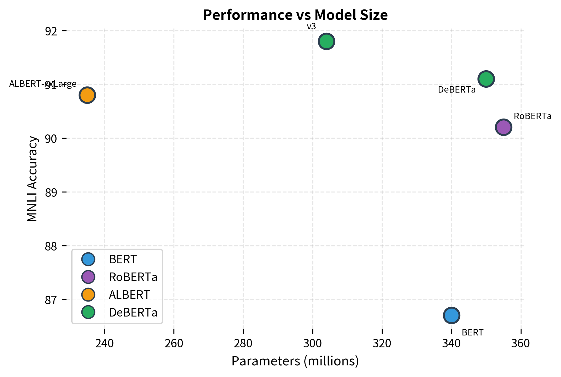
DeBERTa achieved state-of-the-art results on numerous benchmarks when released. Let's examine its performance relative to other BERT variants:
The progression from BERT to DeBERTa-v3 shows steady improvements across all benchmarks. MNLI accuracy improves by over 5 points, while SQuAD v2 gains nearly 10 points. Notably, DeBERTa-v3-Large achieves these results with fewer parameters than RoBERTa-Large, demonstrating that architectural innovations (disentangled attention, EMD, RTD training) can be more effective than simply scaling up.
DeBERTa-v3-Large achieves the best performance across all benchmarks despite having fewer parameters than RoBERTa-Large. The combination of disentangled attention, enhanced mask decoding, and ELECTRA-style pretraining creates a more efficient and effective model.
Computational Considerations
DeBERTa's disentangled attention is more computationally expensive than standard attention. The three attention components each require separate matrix multiplications, roughly tripling the attention computation. However, the improved representational capacity often makes this trade-off worthwhile for challenging NLU tasks.
For latency-sensitive applications, the computational overhead may matter. For offline processing or when accuracy is the priority, DeBERTa's improvements often justify the cost.
Limitations and Impact
DeBERTa's innovations come with trade-offs that affect when and how to use it.
The computational cost of disentangled attention is significant. Computing three separate attention components roughly triples the attention computation compared to standard BERT. For applications where inference latency is critical, such as real-time systems or edge deployment, this overhead may be prohibitive. The performance gains must be weighed against the increased computational budget.
The relative position encoding, while more generalizable than absolute positions, still requires the model to learn position-specific patterns. Very long sequences beyond the training distribution may not benefit from the relative encoding as much as expected. The bounded relative position range (typically 512) means distant tokens share the same position embedding, potentially losing fine-grained positional information.
DeBERTa's Enhanced Mask Decoder adds complexity to the architecture. The additional transformer layers for absolute position injection increase both parameters and computation. For some downstream tasks, particularly those where absolute position is less important, this component may provide diminishing returns.
Despite these limitations, DeBERTa's impact on the field has been substantial. The disentangled attention formulation demonstrated that separating content and position representations improves model expressiveness. This insight influenced subsequent architectures that sought to decouple different aspects of the input representation.
DeBERTa-v3's adoption of ELECTRA-style pretraining showed that the discriminative approach generalizes beyond the original ELECTRA model. By combining disentangled attention with replaced token detection, DeBERTa-v3 achieved efficiency gains that made large-scale pretraining more accessible. The model consistently topped leaderboards on challenging NLU benchmarks, establishing new state-of-the-art results that subsequent models had to beat.
The practical implication is clear: for tasks where accuracy matters more than latency, DeBERTa represents one of the strongest encoder-only models available. Its improvements over BERT and RoBERTa are consistent across diverse benchmarks, making it a reliable choice for demanding NLU applications.
Key Parameters
When working with DeBERTa, these parameters most significantly affect performance and efficiency:
-
max_relative_positions (default: 512): The maximum relative distance encoded with unique embeddings. Positions beyond this distance share embeddings. Larger values capture finer-grained positional information but increase memory for position embeddings.
-
hidden_size (768 for Base, 1024 for Large): The dimension of hidden representations. DeBERTa follows BERT's hidden size conventions. Larger hidden sizes increase model capacity and disentangled attention cost proportionally.
-
num_heads (12 for Base, 16 for Large): Number of attention heads. Each head computes three attention components (c2c, c2p, p2c), so more heads increase both expressiveness and computation.
-
pos_att_type (default: ["c2p", "p2c"]): Which disentangled attention components to include. Can be configured to use only content-to-position or only position-to-content for efficiency, though all components typically yield best results.
-
emd_layers (default: 2): Number of Enhanced Mask Decoder layers. These layers incorporate absolute position information before MLM prediction. More layers add capacity but also parameters and computation.
-
relative_attention (default: True): Whether to use relative position attention. When disabled, falls back to absolute position encoding like BERT.
Summary
DeBERTa introduced several innovations that improved upon BERT's architecture:
-
Disentangled attention separates content and position into distinct representations, then computes three attention components: content-to-content, content-to-position, and position-to-content. This gives the model explicit control over how meaning and location interact during attention.
-
Relative position encoding replaces BERT's absolute positions with relative distances. This generalizes better across sequence lengths and captures the intuition that "two tokens apart" matters more than "at positions 5 and 7."
-
Enhanced Mask Decoder delays absolute position injection until just before MLM prediction. The encoder uses only relative positions, keeping positional signals separate until they're needed for the final prediction.
-
DeBERTa-v2 added n-gram embeddings via convolution, expanded vocabulary size, and scaled to larger models.
-
DeBERTa-v3 adopted ELECTRA-style replaced token detection, training on all tokens rather than just masked ones for improved efficiency.
The combination of these techniques produced a model that consistently outperforms BERT, RoBERTa, and ALBERT on challenging NLU benchmarks. For applications where accuracy justifies additional computation, DeBERTa represents the current state of the art in encoder-only transformers.
Quiz
Ready to test your understanding? Take this quick quiz to reinforce what you've learned about DeBERTa's disentangled attention and architectural innovations.

Comments