Sparse Attention Patterns: Local, Strided & Block-Sparse Approaches

Standard attention computes pairwise scores between all tokens, creating an $n \times n$ attention matrix where $n$ is the sequence length. This quadratic scaling becomes prohibitively expensive for long sequences. Sparse attention offers a principled solution: instead of attending to every position, each token attends only to a carefully chosen subset. The key insight is that most attention weights in practice are small, meaning many token pairs contribute little to the final representation. By restricting attention to positions that matter most, sparse patterns achieve near-linear complexity while preserving the model's ability to capture important relationships.

This chapter explores the fundamental sparse attention patterns that form the building blocks of efficient transformers. We'll implement local windowed attention, strided patterns, and block-sparse attention, then combine them into hybrid approaches used by models like Sparse Transformer, Longformer, and BigBird.

Before diving into specific patterns, let's understand why sparsity works. In natural language, most dependencies are local: a word is most strongly influenced by nearby words. Long-range dependencies exist but are relatively rare. Consider the sentence "The cat that the dog chased ran away." The verb "ran" primarily depends on "cat" (its subject), not on every intervening word. A sparse attention pattern that captures this key dependency while ignoring irrelevant pairs can achieve similar quality to full attention at a fraction of the cost.

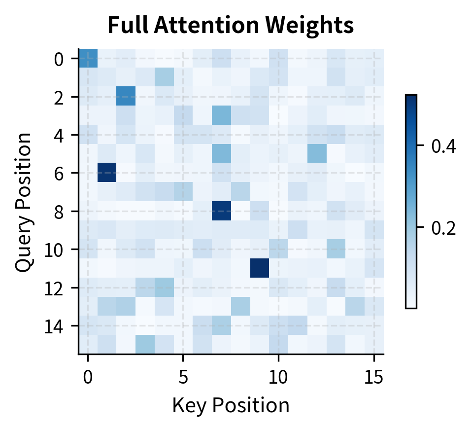
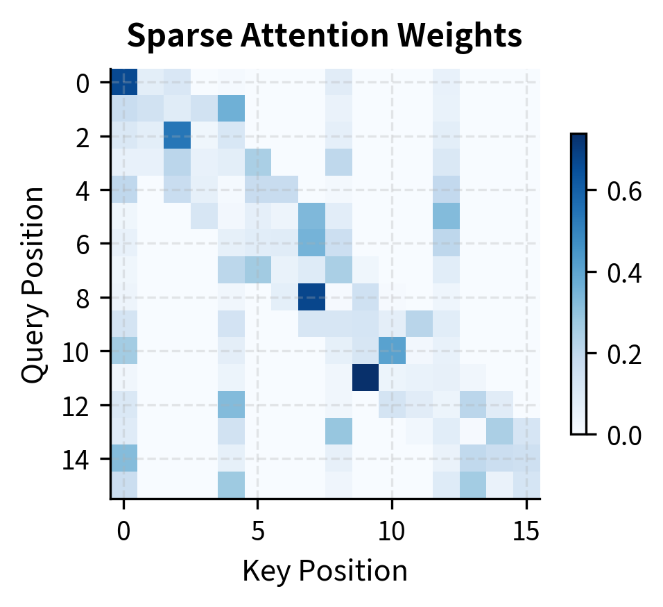
Let's visualize how attention weights are distributed in practice to motivate sparsity.

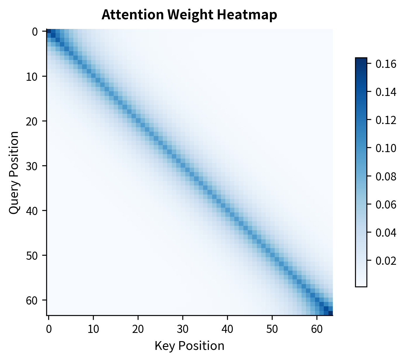
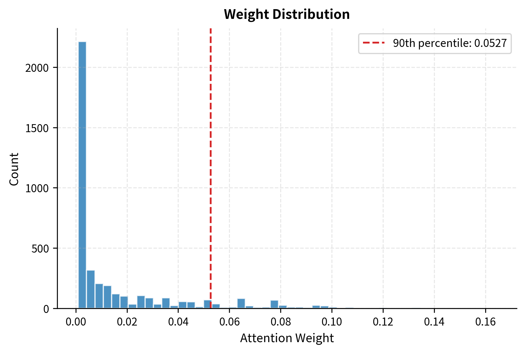
The analysis reveals a key insight: attention weights are highly concentrated. Most of the attention mass falls on a small number of positions per query, while the majority of positions receive negligible weight. This natural sparsity suggests we can skip computing many attention scores without significantly affecting the output.

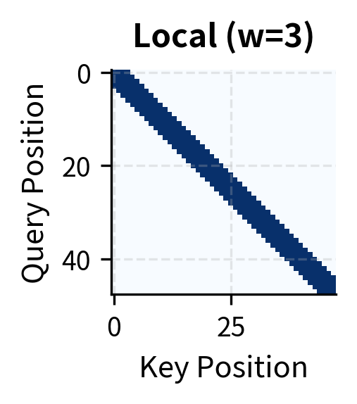
The most intuitive sparse pattern is local attention, where each token attends only to tokens within a fixed window around it. This pattern exploits the locality of language: consecutive words form phrases, sentences have local structure, and most grammatical dependencies span short distances.

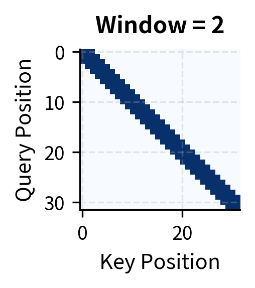
To formalize local attention, we need to answer a simple question: which positions should a token be allowed to attend to? The intuition is straightforward. Imagine you're reading position 10 in a sequence. Local attention says you can "look" at positions 8, 9, 10, 11, and 12 if the window size is 2, but nothing beyond that range. The window creates a neighborhood around each position.

Let's define this precisely. For a window size $w$, each query at position $i$ attends to positions in the range $[i - w, i + w]$. This range includes:

• $w$ positions to the left (earlier in the sequence)
• The current position $i$ itself
• $w$ positions to the right (later in the sequence)

The total number of attended positions is $2w + 1$. Notice something crucial: this count is independent of sequence length $n$. Whether your sequence has 100 tokens or 100,000 tokens, each position still attends to exactly $2w + 1$ neighbors. This independence is what gives local attention its $O(n)$ complexity: $n$ positions, each computing $2w + 1$ attention scores, yields $n \cdot (2w + 1)$ total operations.

Now we need a mechanism to enforce this pattern. In transformer attention, we use an attention mask $M$ that modifies the attention scores before the softmax. The mask for local attention is:

where:

• $M_{ij}$: the mask value applied when query position $i$ attends to key position $j$
• $i$: the query position (which token is asking "what should I attend to?")
• $j$: the key position (a candidate token that might be attended to)
• $w$: the window size (the radius of the local neighborhood)
• $|i - j|$: the absolute distance between positions (how far apart are they?)

The mask works through the attention computation. Recall that standard attention computes:

When $M_{ij} = 0$, the attention score passes through unchanged. When $M_{ij} = -\infty$, adding negative infinity to any finite score produces negative infinity. The softmax function then converts $e^{-\infty} = 0$, effectively blocking query $i$ from attending to key $j$. This elegant mechanism lets us selectively disable attention connections without changing the core attention computation.

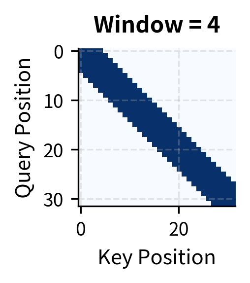
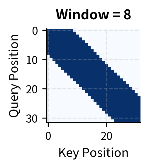
Local attention achieves significant sparsity even with generous window sizes. A window of 8 positions (17 attended positions per query) reduces computation by over 45% for a 32-token sequence. The savings grow with sequence length: for a 4,096-token sequence with window 256, sparsity exceeds 93%.

The optimal window size depends on the task and sequence characteristics. Here are key considerations:

• Linguistic dependencies: Most grammatical dependencies span fewer than 10-15 tokens. A window of 256-512 tokens covers most syntactic structures.
• Task requirements: Sentiment analysis might need only local context, while question answering may require longer-range connections.
• Computational budget: Larger windows provide more context but increase memory and compute proportionally.
• Layer depth: Some architectures use smaller windows in early layers and larger windows (or global attention) in later layers.

The speedup from local attention grows linearly with sequence length. At 32,768 tokens, local attention with a 256-token window provides over 60x speedup compared to full attention. This scaling is what makes local attention essential for processing long documents.

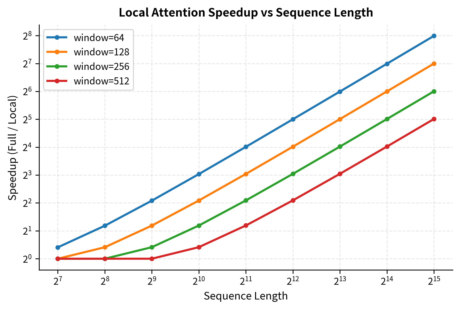
The log-log plot reveals the linear relationship between sequence length and speedup. Doubling the sequence length approximately doubles the speedup, regardless of window size. Smaller windows provide greater speedups but capture less context.

While local attention captures nearby dependencies, it cannot directly model long-range relationships. Strided attention addresses this by having each position attend to positions at regular intervals throughout the sequence. This creates "highways" for information to flow across long distances.

Local attention has a fundamental limitation: it cannot see beyond the window. Position 0 can never directly attend to position 1000, no matter how many attention scores we compute within that single layer. To bridge long distances, we need a different pattern.

The key insight behind strided attention is the concept of hub positions. Think of hubs like train stations in a transit network. Not every location has a direct connection to every other location, but major stations connect to many destinations. Similarly, strided attention designates certain positions as hubs that all other positions can access.

For a stride $s$, we designate every $s$-th position as a hub. With stride $s = 4$, positions 0, 4, 8, 12, 16, ... become hubs. Each query position can attend to:

1. All hub positions: Every position can reach the hubs, creating information highways across the sequence
2. Itself: Self-attention is always preserved so each token can access its own representation

This creates a two-hop connectivity pattern. Consider positions 3 and 97 in a sequence. They cannot directly attend to each other (neither is a hub for typical stride values). But in layer 1, position 3 attends to hub 4, and position 97 attends to hub 96. In layer 2, both hubs can attend to each other (since hubs attend to all other hubs), and information flows between them. After just two layers, any two positions are connected.

The formal mask for strided attention is:

where:

• $M_{ij}$: the mask value when query $i$ considers attending to key $j$
• $s$: the stride parameter (the spacing between hub positions)
• $j \mod s$: the remainder when dividing $j$ by $s$. When this equals 0, position $j$ is a hub
• $j = i$: the self-attention condition, ensuring diagonal connectivity

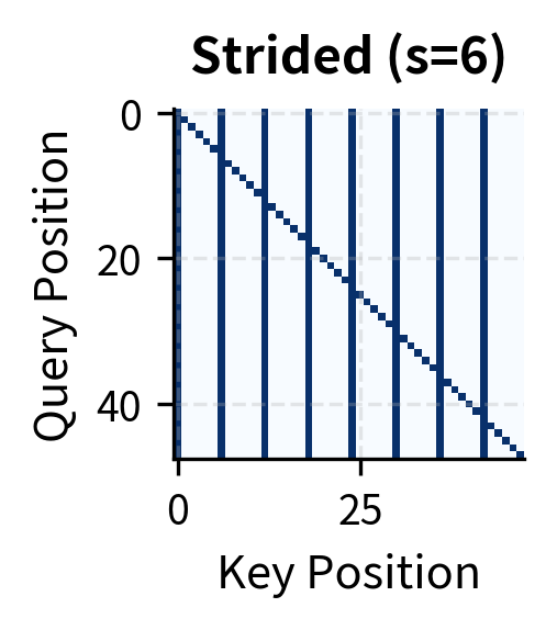
The first condition ($j \mod s = 0$) produces the characteristic vertical stripes in the attention pattern. Every query attends to the same set of hub columns, creating shared access points. The second condition ($j = i$) adds the diagonal, ensuring self-attention. Together, these conditions guarantee that information can propagate across any distance in two hops, while keeping the number of attended positions per query at approximately $n/s + 1$, where $n$ is sequence length.

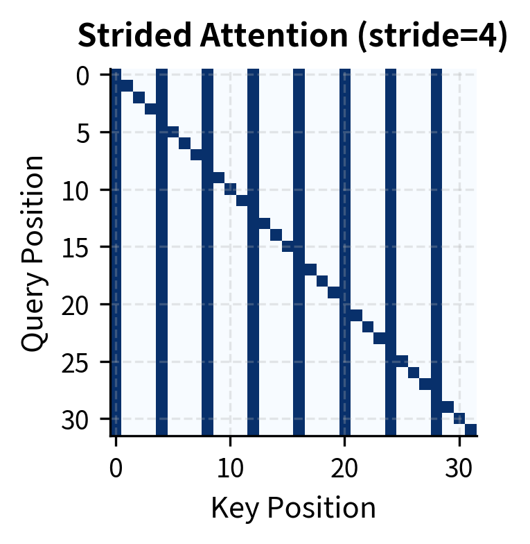
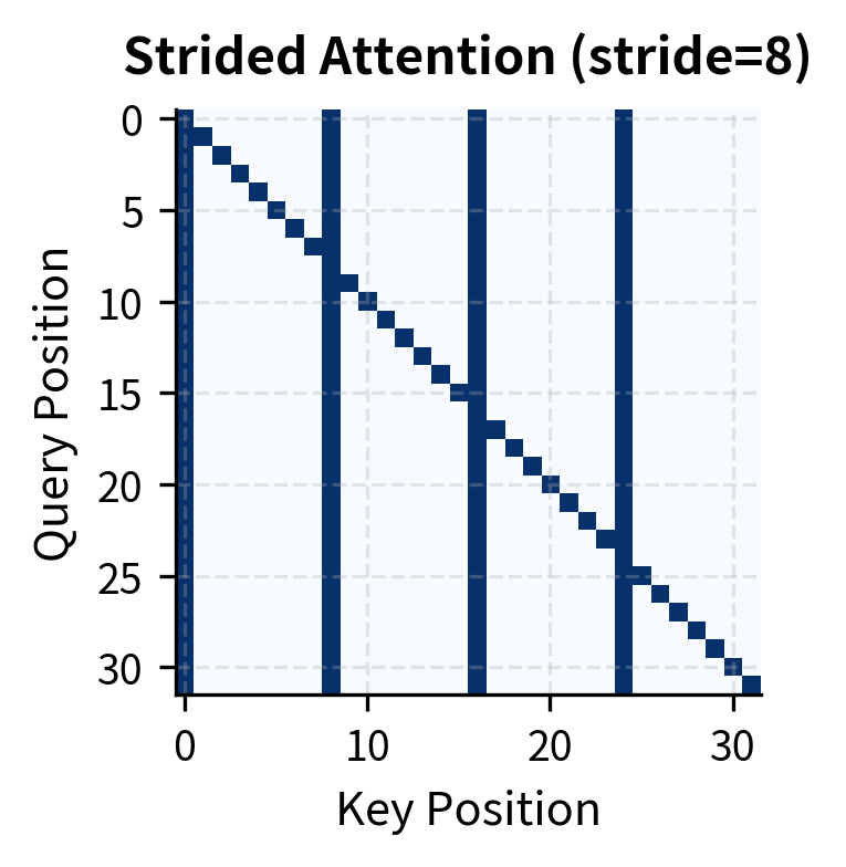
Strided attention creates a distinctive pattern: vertical columns at hub positions (which all queries attend to) and a diagonal for self-attention. The hub positions act as relay points, allowing information to propagate across the sequence in two hops: any position can reach a hub, and from the hub, information flows to other positions in subsequent layers.

A key property of strided attention is the maximum "hop distance" between any two positions. With stride $s$:

• Any position is at most $s/2$ steps from a hub position
• In one attention layer, information can travel to a hub
• In the next layer, it can travel from the hub to any other position

This means any two positions are connected within 2 layers, regardless of their distance in the sequence. This is significantly better than local attention, which requires $O(n/w)$ layers to connect distant positions, where $n$ is the sequence length and $w$ is the window size.

After just 2 layers of strided attention, every position can reach every other position. This demonstrates the power of strided patterns for long-range information flow, achieving global connectivity with sparse local computation.

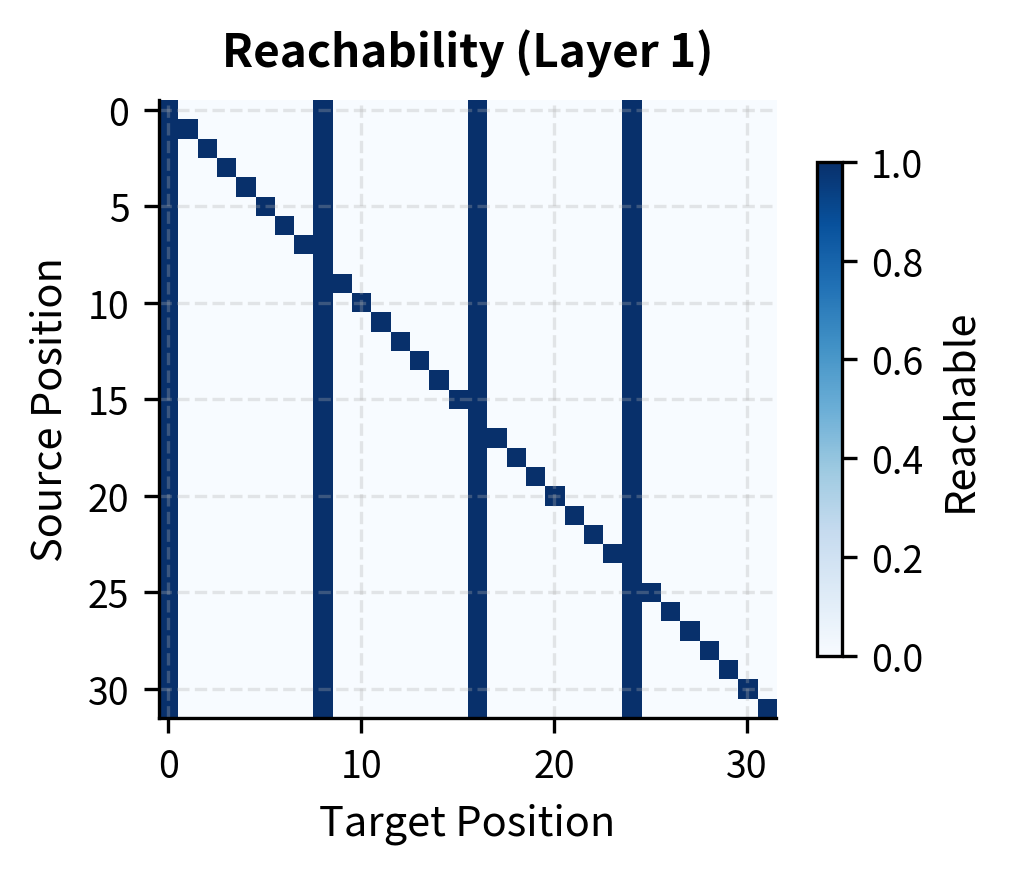
The visualization shows how reachability expands with depth. After layer 1, we see the strided pattern: each position reaches hubs (vertical stripes) and itself (diagonal). After layer 2, the matrix is fully connected, demonstrating that any position can reach any other position through an intermediate hub.

Block-sparse attention groups positions into blocks and defines attention patterns at the block level. This approach is particularly hardware-friendly because modern GPUs and TPUs are optimized for matrix operations on contiguous memory blocks.

The patterns we've seen so far, local and strided, define attention at the level of individual positions. Block-sparse attention takes a different approach: it groups positions into contiguous blocks and defines attention at the block level. This abstraction has a practical motivation. Modern GPUs are designed to process data in aligned, contiguous chunks. By organizing attention into blocks that match hardware execution units, we can achieve theoretical speedups in actual wall-clock time.

Imagine dividing a 1024-token sequence into blocks of size $b = 64$. This creates $1024/64 = 16$ blocks. Instead of asking "which of 1024 positions can position $i$ attend to?", we ask "which of 16 blocks can block $B_i$ attend to?" This coarser-grained question has fewer possible answers, and each answer involves a dense $64 \times 64$ matrix operation that GPUs handle efficiently.

The key parameters for block-sparse attention are:

• $b$: the block size (number of positions per block)
• $k$: the number of blocks each query block attends to

If we select $k$ blocks for each query block, the complexity analysis proceeds as follows:

1. Number of query blocks: The sequence divides into $n/b$ blocks
2. Attention per query block: Each block attends to $k$ other blocks
3. Operations per block pair: Computing attention between two blocks of size $b$ requires $b \times b = b^2$ score computations

Multiplying these together:

When $k$ and $b$ are constants independent of $n$, this expression is linear in sequence length. The quadratic term has vanished. Even better, each $b \times b$ block attention can use highly optimized dense matrix multiplication routines, achieving near-peak GPU utilization.

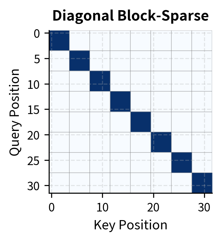
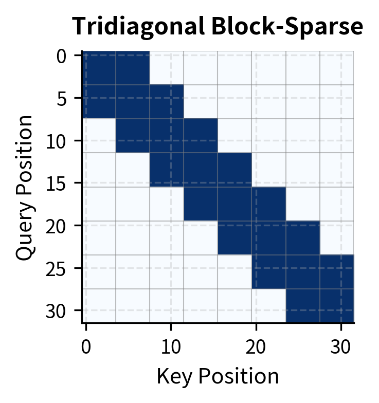
Block-sparse attention provides a clean abstraction for hardware-efficient implementation. The regular block structure maps directly to GPU thread blocks, enabling efficient parallel execution with minimal memory overhead.

The advantage of block-sparse attention goes beyond theoretical complexity. Modern GPUs achieve peak performance when operating on aligned, contiguous memory blocks. Random sparse patterns, while mathematically equivalent, suffer from irregular memory access patterns that underutilize hardware.

Block-sparse attention can be 3x or more efficient than random sparse patterns at the same sparsity level. This hardware awareness is crucial for practical implementations and explains why production models favor structured sparsity.

Real-world efficient attention mechanisms combine multiple patterns to balance local context, global reach, and computational efficiency. The Sparse Transformer paper introduced the idea of factorizing attention across multiple heads, with different heads using different patterns.

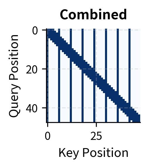
The most common combination pairs local attention for nearby tokens with strided attention for long-range connections. Together, they ensure every pair of positions can communicate within a small number of layers while maintaining overall sparsity.

An elegant approach from Sparse Transformer assigns different patterns to different attention heads. Half the heads might use local attention while the other half use strided attention. This factorization allows the model to learn which pattern is most useful for different types of dependencies.

Factorized attention provides flexibility: local heads handle nearby dependencies while strided heads capture long-range patterns. The model learns to route information through the appropriate heads during training.

Having established the theory behind sparse patterns, let's implement a complete sparse attention module. This implementation prioritizes clarity over performance, demonstrating how the mask-based approach works in practice. Understanding this foundation will help you work with optimized libraries like xformers or Flash Attention later.

Sparse attention follows the same computational structure as standard attention, with one addition: we apply a mask before the softmax to block certain attention connections. The algorithm proceeds in four steps:

1. Compute raw attention scores: Multiply queries by keys to get similarity scores
2. Apply the sparse mask: Set blocked positions to $-\infty$ (we use $-10^9$ numerically)
3. Softmax normalization: Convert scores to probability weights (blocked positions become zero)
4. Weighted sum: Combine values according to the attention weights

Let's implement each step:

To validate our implementation and demonstrate the effectiveness of sparse patterns, let's compare the outputs of full attention versus a combined local + strided pattern:

The difference between full and sparse attention outputs is relatively small, even though sparse attention computes far fewer pairs. This validates the core principle behind sparse attention: most attention scores contribute little to the final output, so we can skip computing them without significantly degrading the representation quality.

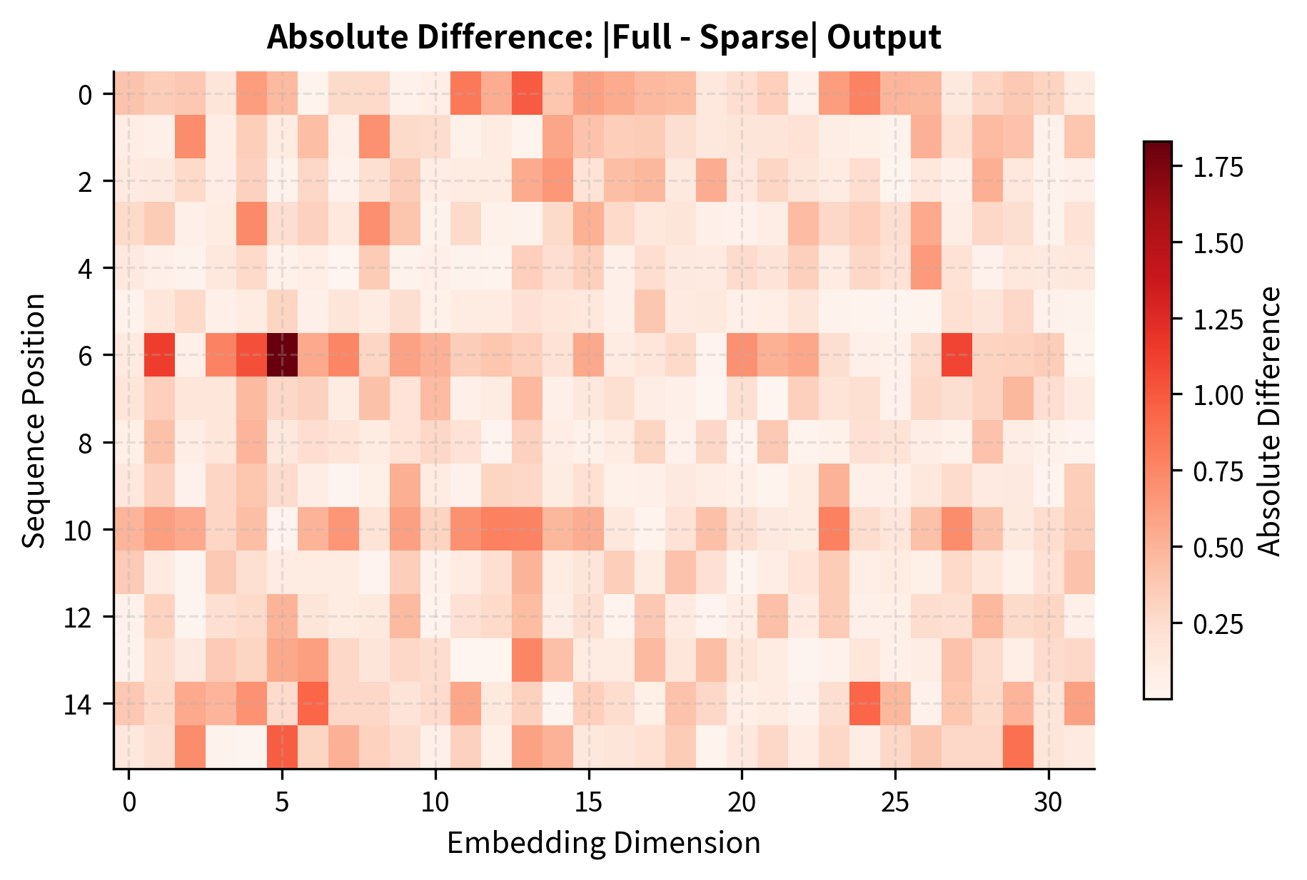
The heatmap reveals that differences are distributed across all positions, but remain small. This uniform distribution suggests that sparse attention doesn't systematically fail for any particular positions; rather, it introduces small approximation errors throughout the sequence.

Let's verify the computational savings from sparse attention empirically.

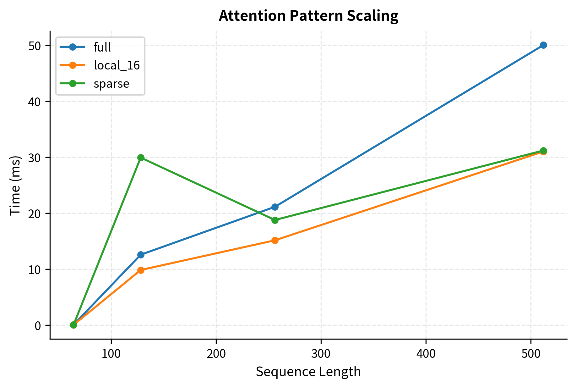
The benchmark confirms the theoretical complexity analysis: sparse patterns scale better than full attention, with the advantage growing as sequence length increases. Note that our NumPy implementation doesn't fully exploit sparsity since it still computes the full matrix before masking. Production implementations using optimized sparse kernels would show even larger speedups.

When implementing sparse attention in practice, several factors influence the choice of pattern and parameters.

Different tasks and sequence lengths call for different patterns:

• Short sequences (less than 512 tokens): Full attention is often fast enough. Sparse patterns may not provide significant benefit and add implementation complexity.
• Medium sequences (512 to 2048 tokens): Local attention with a window of 128-256 tokens works well for most tasks. Add strided or global attention for tasks requiring long-range dependencies.
• Long sequences (more than 2048 tokens): Combined patterns are essential. Consider factorized attention across heads or hierarchical approaches.

Sparse attention reduces both memory and compute, but the savings differ:

• Compute: Scales directly with sparsity. 90% sparsity means 10x fewer FLOPs.
• Memory: Storing the sparse mask adds overhead. For very sparse patterns, mask storage can dominate for short sequences.

For high sparsity (95%+) and long sequences, sparse storage provides significant memory savings. However, for shorter sequences or moderate sparsity, the overhead of sparse formats can negate the benefits.

Sparse attention patterns can affect gradient flow during training. Positions that are never attended to receive no gradient signal through attention. This is typically acceptable when patterns ensure every position is reachable within a few layers, but can cause issues with overly aggressive sparsity.

The key insight is that multi-layer transformers compose attention patterns. Even if layer 1 uses sparse attention, the effective receptive field grows with depth. A position unreachable in one layer may become reachable through intermediate positions in subsequent layers.

Sparse attention patterns represent a fundamental advance in efficient transformer design, enabling the processing of sequences that would be impossible with full attention. However, they come with trade-offs that practitioners must understand.

The most significant limitation is the potential loss of long-range dependencies. While patterns like local + strided ensure connectivity, they may not capture all important relationships as effectively as full attention. Tasks requiring precise long-range reasoning, such as mathematical proofs or complex code understanding, may suffer from aggressive sparsity. The solution often involves tuning the pattern parameters: larger windows, smaller strides, or additional global tokens to ensure critical positions remain connected.

Implementation complexity is another practical concern. While conceptually simple, efficient sparse attention requires careful memory management and often custom CUDA kernels to achieve the theoretical speedups. Libraries like xformers and Flash Attention provide optimized implementations, but integrating them into existing codebases requires effort. The block-sparse approach helps here by mapping to hardware-friendly operations, but still requires infrastructure beyond standard dense attention.

Despite these challenges, sparse attention patterns have enabled a new generation of long-context models. Longformer, BigBird, and their successors process documents, books, and codebases that were previously inaccessible to transformers. The efficiency gains are substantial: processing a 4,096-token document with sparse attention uses roughly the same resources as a 512-token document with full attention. This has opened new applications in document understanding, long-form generation, and multi-turn conversation.

Sparse attention patterns address the quadratic complexity bottleneck of standard attention by restricting each query to attend to a subset of keys. The key patterns are:

• Local attention: Each position attends to a fixed window of nearby tokens, exploiting the locality of language. Complexity is $O(n \cdot w)$ where $n$ is the sequence length and $w$ is the window size.

• Strided attention: Positions attend to regularly-spaced hub positions, enabling long-range information flow within two hops. Complexity is $O(n \cdot n/s)$ where $s$ is the stride, creating highways for information propagation across long sequences.

• Block-sparse attention: Groups positions into blocks of size $b$ and defines attention at the block level. Complexity is $O(n \cdot k \cdot b)$ where $k$ is the number of blocks attended to. Hardware-friendly due to regular memory access patterns.

• Combined patterns: Real systems combine multiple patterns, often using factorized multi-head attention where different heads use different patterns.

The effectiveness of sparse attention rests on a key observation: most attention weights are small, concentrated on a few important positions. By carefully selecting which positions to attend to, sparse patterns preserve most of the representational power of full attention while dramatically reducing computational cost.

These building blocks form the foundation for efficient attention mechanisms like Longformer, BigBird, and Sparse Transformer. The next chapters explore specific architectures that combine sparse patterns with additional techniques like sliding windows and global tokens to achieve even better trade-offs between efficiency and expressiveness.

When implementing sparse attention patterns, several parameters control the trade-off between efficiency and model quality:

• window_size: The number of positions each query attends to on each side in local attention. Larger windows capture more context but increase computation. Typical values range from 64 to 512 tokens. Start with 256 for most tasks and adjust based on whether the model struggles with local dependencies.

• stride: The interval between hub positions in strided attention. Smaller strides provide denser global connectivity but increase computation. Common values are 8 to 64. A stride of $\sqrt{n}$ (where $n$ is sequence length) balances coverage and efficiency.

• block_size: The size of contiguous blocks in block-sparse attention. Must be chosen to align with GPU warp sizes (typically 32 or 64) for optimal hardware utilization. Larger blocks reduce indexing overhead but coarsen the sparsity pattern.

• sparsity_ratio: The fraction of attention pairs that are masked out. Higher sparsity (0.9+) dramatically reduces computation but may degrade quality on tasks requiring dense interactions. Monitor validation loss when increasing sparsity.

• num_heads: In factorized multi-head attention, determines how many heads use each pattern type. Splitting evenly between local and strided heads works well as a starting point. Models may benefit from more local heads for tasks with strong locality.

• pattern: The combination strategy for multiple sparse patterns. Options include union (OR), which is most common, or alternating patterns across layers. The union approach ensures positions blocked by one pattern may still be reached through another.

Ready to test your understanding? Take this quick quiz to reinforce what you've learned about sparse attention patterns and their role in efficient transformer design.