Sinusoidal Position Encoding: How Transformers Know Word Order

The transformer's self-attention mechanism is permutation invariant: it produces the same output regardless of token order. To capture sequential structure, we need to inject position information. The original "Attention Is All You Need" paper introduced sinusoidal position encoding, an elegant solution that encodes each position as a unique pattern of sine and cosine waves at different frequencies.

This approach offers several compelling properties. Each position receives a deterministic, unique encoding without any learned parameters. The encoding can represent positions the model has never seen during training. And remarkably, relative positions can be computed through simple linear transformations of absolute positions. Let's understand how this works.

Before diving into the mathematics, let's consider what properties we want from a position encoding. We need a function that takes a position index and produces a vector, and this function must satisfy several constraints:

1. Uniqueness: Each position must map to a distinct vector. If positions 5 and 17 produce the same encoding, the model cannot distinguish them.

2. Bounded values: The encoding should not grow unboundedly with position. If position 1000 produces values 1000 times larger than position 1, the position signal would overwhelm the semantic content of the embeddings.

3. Smooth progression: Nearby positions should have similar encodings. Position 50 should be more similar to position 51 than to position 500, giving the model useful gradient information.

4. Deterministic: The same position should always produce the same encoding, without requiring any learned parameters.

Sinusoidal functions satisfy all these requirements elegantly. Sine and cosine oscillate smoothly between -1 and 1, ensuring bounded values. Different frequencies distinguish positions at different scales. And the encoding is purely deterministic, computed from a fixed formula.

The core idea is to assign each position a unique "fingerprint" using waves of different frequencies. Think of how you might describe your location in a building: you could give the floor number (coarse scale), the room number (medium scale), and your position within the room (fine scale). Together, these scales uniquely identify any location.

For position encoding, we use sine and cosine waves at different frequencies to achieve the same multi-scale identification. Each position $pos$ in the sequence receives a $d$-dimensional vector, where consecutive pairs of dimensions use sine and cosine at the same frequency:

where:

• $pos$: the position index in the sequence (0, 1, 2, ...)
• $i$: the dimension index pair (0, 1, 2, ..., $d/2 - 1$)
• $d$: the total embedding dimension
• $PE_{(pos, 2i)}$: the encoding value at position $pos$, even dimension $2i$
• $PE_{(pos, 2i+1)}$: the encoding value at position $pos$, odd dimension $2i+1$
• $10000$: a base constant that controls the frequency range

The key to the formula is the denominator $10000^{2i/d}$. This term controls how fast each dimension pair oscillates as position increases. Let's unpack what happens at different dimension indices:

• When $i = 0$ (the first dimension pair): The denominator is $10000^0 = 1$, so we compute $\sin(pos)$ and $\cos(pos)$. This oscillates rapidly: moving from position 0 to position 6 covers roughly one full cycle.

• When $i = d/2 - 1$ (the last dimension pair): The denominator is approximately $10000^1 = 10000$, so we compute $\sin(pos/10000)$ and $\cos(pos/10000)$. This oscillates extremely slowly: you need 62,832 positions to complete one full cycle.

The exponent $2i/d$ creates a geometric progression of frequencies. As $i$ increases from 0 to $d/2 - 1$, the exponent increases from 0 to approximately 1, and the denominator grows from 1 to 10000. This exponential scaling ensures that each dimension pair captures position information at a different resolution.

Each dimension pair uses both sine and cosine at the same frequency. This pairing is not arbitrary; it serves two purposes:

1. Unique identification within a cycle: Sine alone cannot distinguish positions that differ by multiples of $2\pi$. But the (sine, cosine) pair at any frequency uniquely identifies a phase angle. Geometrically, as position increases, the (sin, cos) pair traces a circle in 2D space, and every point on that circle corresponds to a unique position within one cycle.

2. Enabling relative position computation: The sine/cosine pairing allows relative positions to be computed through rotation matrices, a property we'll explore in detail later. This mathematical structure means the model can potentially learn to attend to relative positions using simple linear operations.

Now that we have the formula, let's build deeper intuition for why this multi-frequency approach works so well. The key insight is that different dimensions encode position at different scales, much like how we represent time using multiple units.

Consider a clock with both a second hand and an hour hand. The second hand rotates rapidly, completing one cycle per minute. If you only had the second hand, you could tell the difference between 3:00:15 and 3:00:45, but you couldn't distinguish 3:00:15 from 4:00:15, since both would show the second hand at the same position. The hour hand solves this problem: it moves slowly, completing one cycle every 12 hours, so it can distinguish times that the second hand cannot.

Sinusoidal position encoding applies the same principle. The first dimension pairs oscillate rapidly (like the second hand), distinguishing nearby positions with high precision. The later dimension pairs oscillate slowly (like the hour hand), distinguishing distant positions that the fast oscillators cannot. Together, they create a multi-resolution representation where any two positions, no matter how close or far apart, can be distinguished by at least one dimension pair.

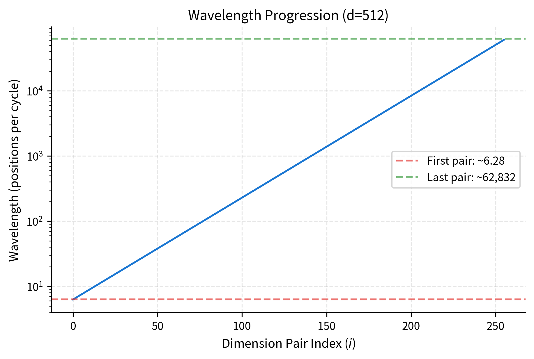
The wavelength formula makes this precise. For dimension pair $i$, the wavelength (the number of positions needed for one complete oscillation cycle) is:

where:

• $\lambda_i$: the wavelength for dimension pair $i$ (measured in positions per cycle)
• $10000^{2i/d}$: the frequency denominator that grows geometrically with $i$
• $2\pi$: the angular measure of one complete cycle (in radians)

This formula reveals the geometric progression at the heart of sinusoidal encoding:

• First dimension pair ($i = 0$): Wavelength is $2\pi \approx 6.28$ positions. Positions 0 through 6 span roughly one full cycle. This fast oscillation distinguishes positions that differ by just 1 or 2.

• Middle dimension pairs: Wavelengths grow exponentially. By the time we reach the middle dimensions, wavelengths might be in the hundreds, suitable for distinguishing positions that differ by tens or hundreds.

• Last dimension pair ($i = d/2 - 1$): Wavelength is approximately $2\pi \cdot 10000 \approx 62,832$ positions. You'd need over 10,000 positions to complete one cycle. This slow oscillation can distinguish positions separated by thousands.

The geometric progression is deliberate and essential. If wavelengths grew linearly, nearby dimension pairs would be redundant, both distinguishing roughly the same positional differences. The exponential growth ensures each dimension pair contributes unique positional information at its own characteristic scale, creating a compact representation that efficiently covers all possible position differences.

The geometric spacing is deliberate. If wavelengths grew linearly, nearby dimension pairs would be redundant. The exponential growth ensures each dimension pair contributes unique positional information.

With the formula and wavelength intuition in place, let's see what sinusoidal position encodings actually look like. We'll implement the encoding from scratch and visualize the resulting patterns to verify that our intuitions match reality.

Position 0 always has sine values of 0 and cosine values of 1 in the first few dimensions. As position increases, the high-frequency dimensions (small indices) change rapidly while low-frequency dimensions (large indices) change slowly.

Let's visualize the encoding as a heatmap to see the wave patterns:

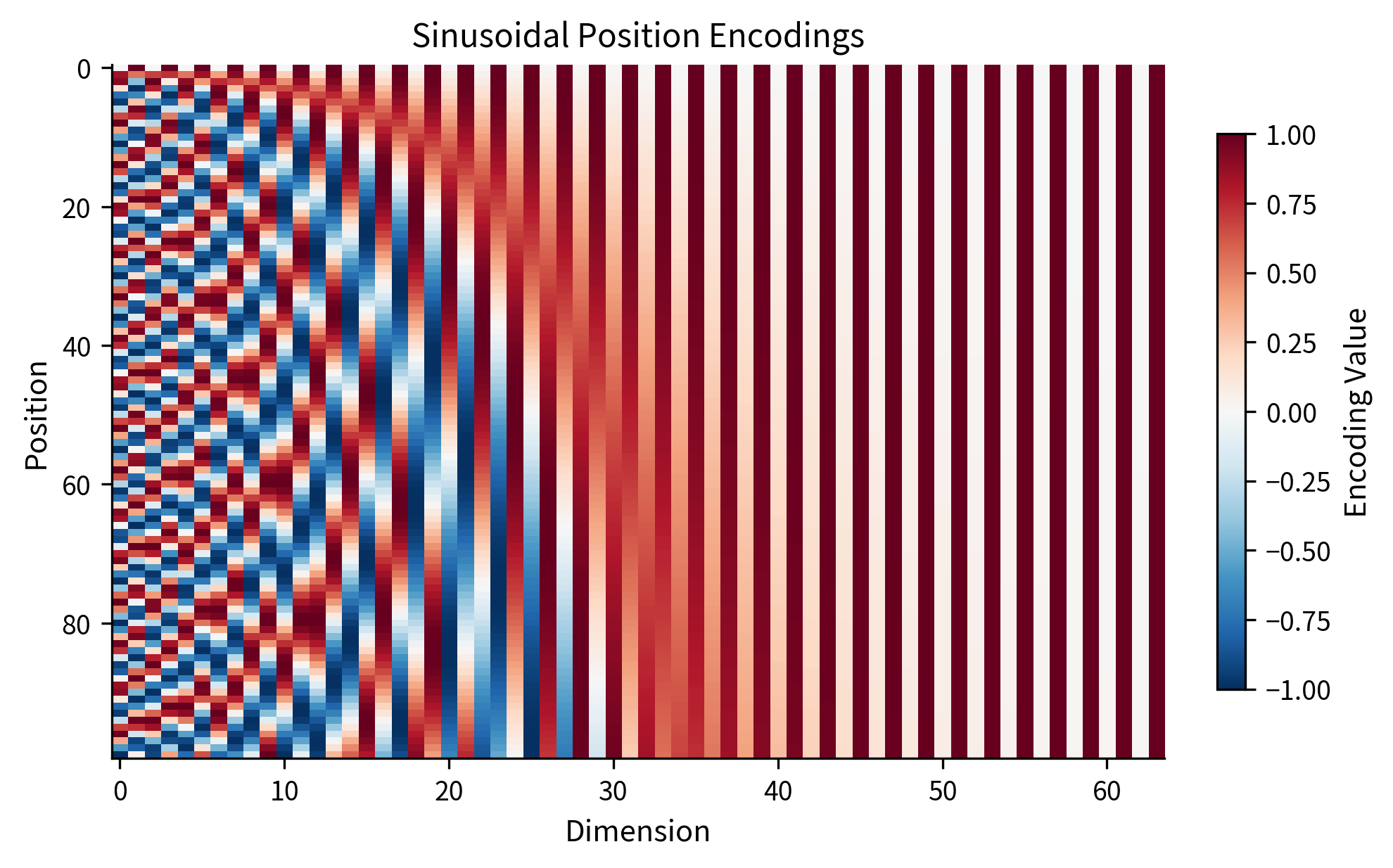
The heatmap reveals the core structure. On the left side (low dimension indices), we see rapid oscillations: positions 0 and 3 might look similar here, but positions 0 and 1 are clearly different. On the right side (high dimension indices), the oscillations are so slow that the entire 100-position range barely covers a fraction of one cycle. The combination ensures every position has a unique encoding.

Let's examine specific dimension pairs to see the sine/cosine relationship:

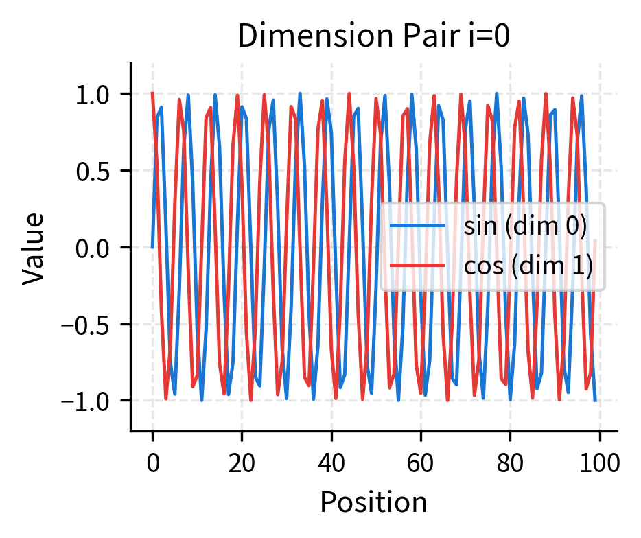
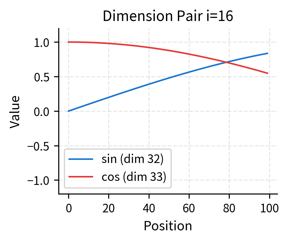
Each dimension pair contributes a (sine, cosine) tuple that traces a circle in 2D space as position increases. The sine and cosine are 90° out of phase, ensuring that every position has a unique combination even within a single dimension pair.

To make this geometric interpretation concrete, let's plot the trajectory of (sin, cos) pairs as position increases:

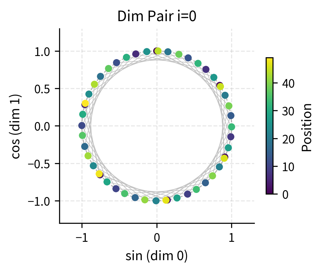
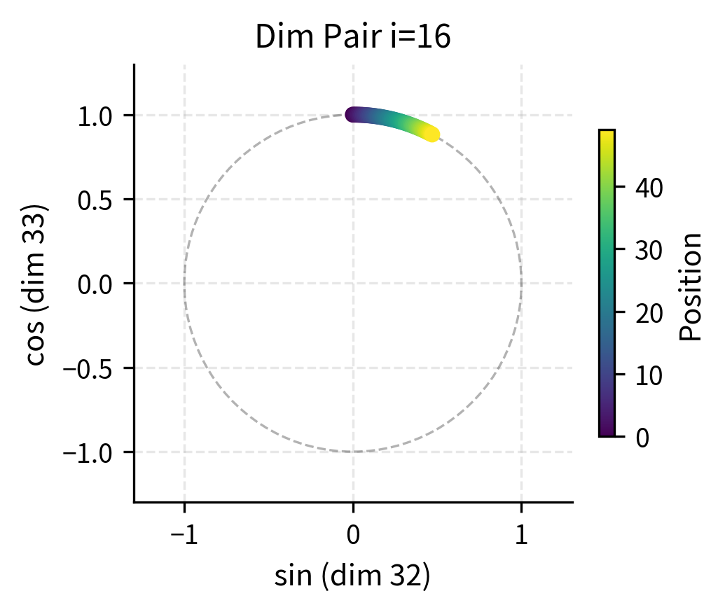
The circular trajectories reveal why sine/cosine pairing works so well. In the first dimension pair (left), the fast oscillation means positions loop around the circle multiple times. Even if two positions land at similar angles on the circle, they'll be distinguished by other dimension pairs with different frequencies. In the middle dimension pair (right), positions are spread across a smaller arc, providing coarse-grained discrimination.

Why does this encoding give each position a unique vector? Consider two positions $pos_1$ and $pos_2$. For them to have identical encodings, they would need to be indistinguishable across all dimension pairs. But with the geometric progression of wavelengths, this is virtually impossible.

If two positions differ by 1, the first dimension pair (wavelength ~6) will clearly distinguish them. If they differ by 100, middle dimension pairs will distinguish them. If they differ by 10,000, the later dimension pairs will distinguish them. The multi-scale representation captures position differences at any granularity.

Let's verify this by computing distances between position encodings:

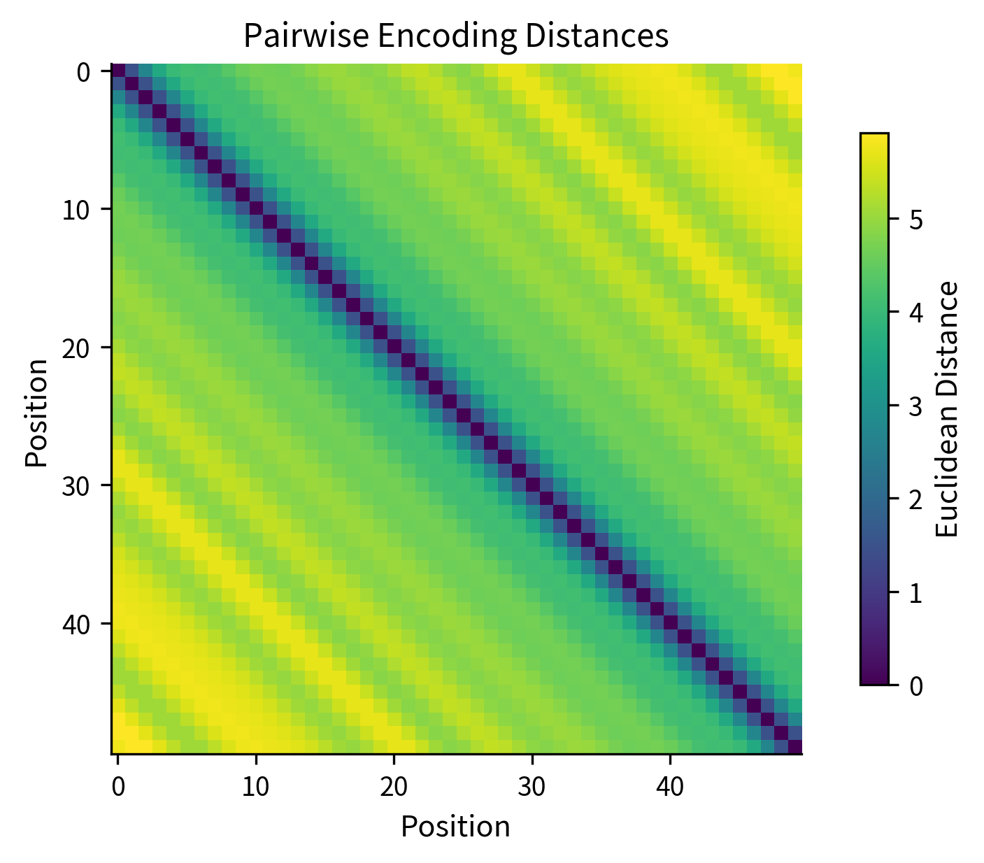
The distance matrix confirms that no two positions have identical encodings (no zeros off the diagonal). The banded structure shows that nearby positions have smaller distances, while distant positions have larger distances. This smooth distance gradient helps the model learn position-dependent patterns.

Let's examine how distance varies with positional separation more precisely:

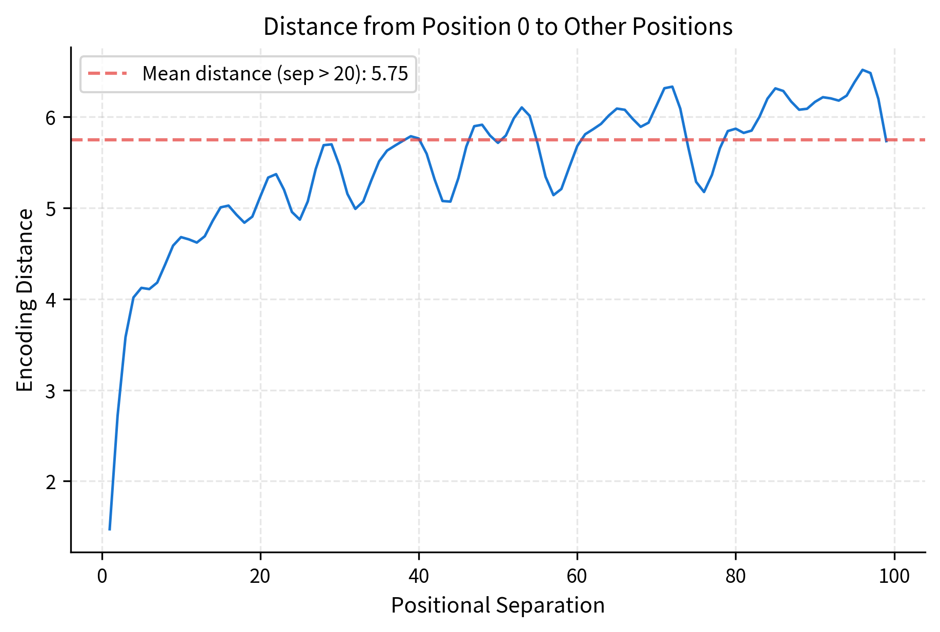
The plot reveals an important property: distance grows quickly for small separations (positions 1-10 are clearly distinguishable from position 0) but then oscillates around a plateau for larger separations. The oscillation comes from the sinusoidal structure: at certain separations, the high-frequency dimensions happen to cycle back to similar values, temporarily reducing the distance. However, the low-frequency dimensions ensure that even these "aliased" positions remain distinguishable.

One of the most elegant properties of sinusoidal encoding is that relative positions can be expressed as linear transformations. For any fixed offset $k$, there exists a matrix $M_k$ such that:

where:

• $PE_{pos}$: the position encoding vector at position $pos$ (a $d$-dimensional row vector)
• $PE_{pos+k}$: the position encoding vector at position $pos + k$
• $M_k$: a $d \times d$ transformation matrix that depends only on the offset $k$, not on the absolute position

This means the model can learn to attend to relative positions (e.g., "the word 3 positions back") using simple linear operations.

To understand why this works, we need to derive the relationship step by step using trigonometric identities.

Step 1: Recall the angle addition formulas. For any angles $a$ and $b$, trigonometry gives us:

where $a$ and $b$ are any angles (in radians). These identities let us express the sine or cosine of a sum in terms of the sines and cosines of the individual angles.

Step 2: Define the angular frequency. For dimension pair $i$, we define the angular frequency as:

where:

• $\omega_i$: the angular frequency for dimension pair $i$ (determines how fast this dimension oscillates)
• $i$: the dimension pair index (0, 1, 2, ..., $d/2 - 1$)
• $d$: the total embedding dimension
• $10000^{2i/d}$: the denominator that grows geometrically with $i$

This means the encoding at position $pos$ in dimension pair $i$ uses the argument $\omega_i \cdot pos$.

Step 3: Apply the addition formulas. To find the encoding at position $pos + k$, we substitute $a = \omega_i \cdot pos$ and $b = \omega_i \cdot k$ into the angle addition formulas:

where:

• $\omega_i = 1/10000^{2i/d}$: the angular frequency for dimension pair $i$
• $pos$: the current position in the sequence
• $k$: the position offset we want to shift by
• $\sin(\omega_i \cdot pos)$ and $\cos(\omega_i \cdot pos)$: the original encoding values at position $pos$ (these are $PE_{(pos, 2i)}$ and $PE_{(pos, 2i+1)}$)
• $\sin(\omega_i k)$ and $\cos(\omega_i k)$: constants that depend only on the offset $k$, not on the absolute position

Step 4: Recognize the matrix structure. The key insight is that the right-hand sides of both equations are linear combinations of $\sin(\omega_i \cdot pos)$ and $\cos(\omega_i \cdot pos)$. This is exactly what matrix multiplication does! We can write:

This is a rotation in 2D! For each dimension pair, the encoding at $pos + k$ is the encoding at $pos$ rotated by angle $\omega_i k$. The rotation matrix for offset $k$ in dimension pair $i$ is:

where:

• $R_k^{(i)}$: the 2×2 rotation matrix for dimension pair $i$ with offset $k$
• $\omega_i = 1/10000^{2i/d}$: the angular frequency for dimension pair $i$
• $k$: the position offset (how many positions to shift)
• $\omega_i k$: the rotation angle, which depends on both the offset and the dimension's frequency

Step 5: Construct the full transformation matrix. The full transformation matrix $M_k$ is block-diagonal, with each 2×2 block being the rotation matrix for that dimension pair:

where:

• $M_k$: the full $d \times d$ transformation matrix for offset $k$
• $R_k^{(i)}$: the 2×2 rotation matrix for dimension pair $i$ (defined above)
• $0$: 2×2 zero matrices (indicating no interaction between dimension pairs)
• The matrix has $d/2$ blocks along the diagonal

This block-diagonal structure means relative position shifts act independently on each dimension pair, rotating the (sine, cosine) pair by an amount proportional to the offset. The independence is crucial: each dimension pair encodes position at its own frequency, and shifting by $k$ positions rotates each pair by its own characteristic angle $\omega_i k$.

Let's verify this property numerically:

The errors are at machine precision, confirming that the relative position property holds exactly. This mathematical structure is what allows transformers to potentially learn relative position relationships through their linear attention projections.

Let's visualize this rotation property for a single dimension pair. We'll show how applying the rotation matrix to an encoding at position $pos$ produces the encoding at position $pos + k$:

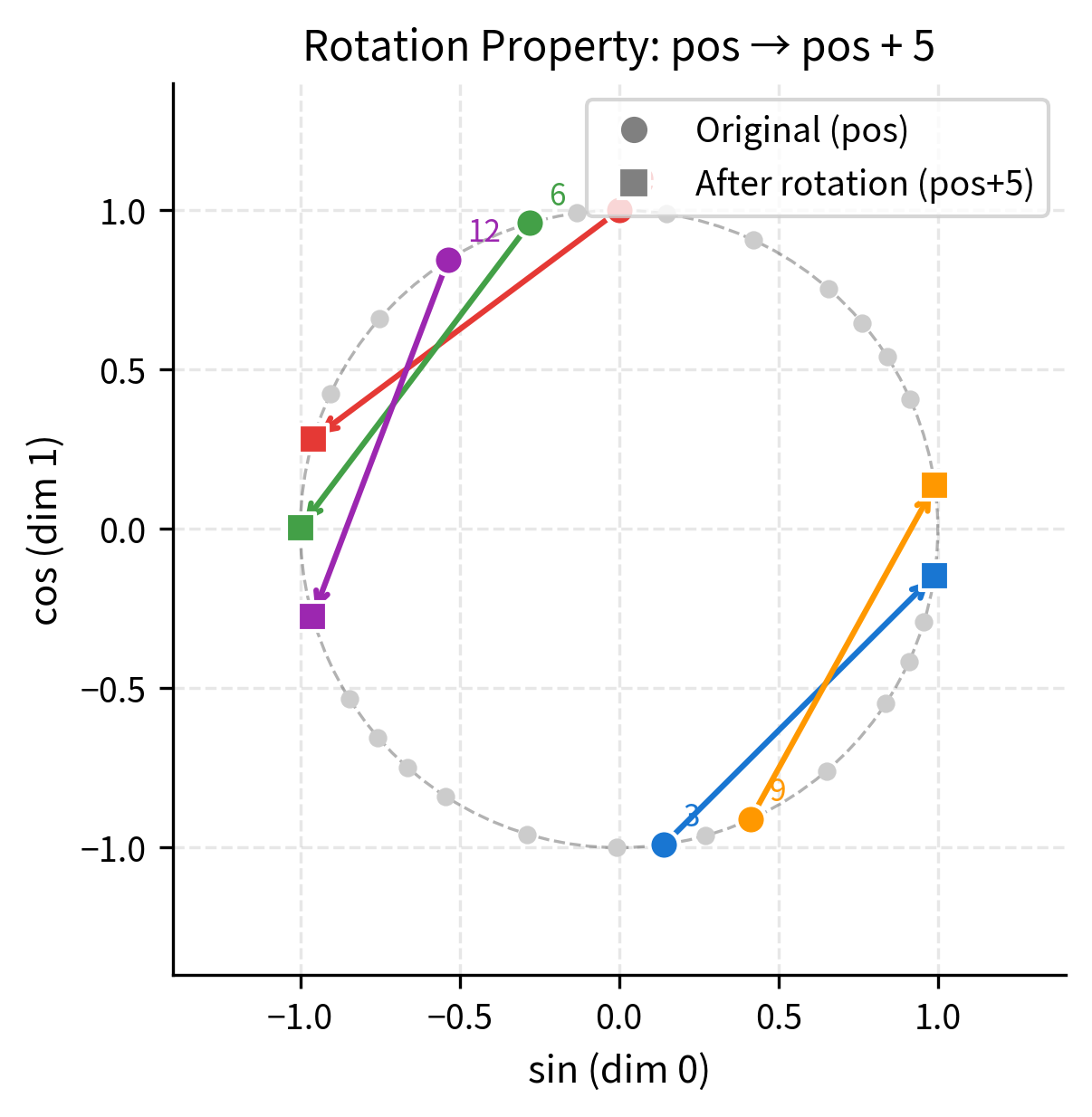
The visualization makes the rotation property tangible. Each colored arrow shows the transformation from position $pos$ (circle) to position $pos + 5$ (square). Notice that all arrows rotate by the same angle, confirming that the transformation depends only on the offset $k$, not on the starting position. This is the geometric essence of how sinusoidal encodings enable learning of relative positions.

A significant advantage of sinusoidal encodings is their ability to represent positions never seen during training. Unlike learned position embeddings that require a fixed vocabulary of positions, sinusoidal encodings are computed from a deterministic formula that works for any position.

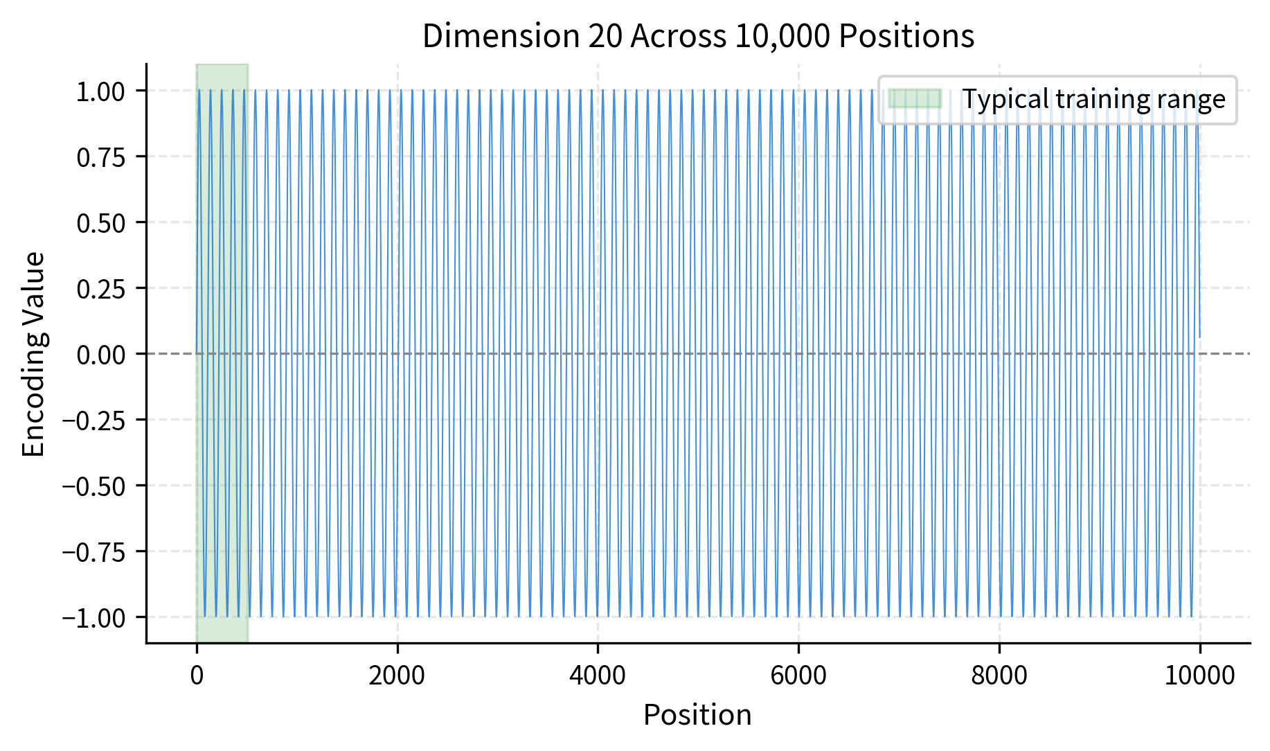
Let's examine how encodings behave beyond typical training lengths:

The encodings remain well-behaved even at position 9,999. Each dimension independently oscillates between -1 and 1, so the encoding never explodes or vanishes. This stability makes sinusoidal encodings suitable for tasks requiring longer contexts than seen during training.

However, extrapolation has a subtle limitation. While the encodings themselves are mathematically valid for any position, the model's attention patterns are learned on sequences of a particular length distribution. If the model trains on sequences of length 512, it has never seen the specific encoding patterns that occur at position 5000. The attention mechanism might not generalize well to these unseen patterns, even though the encodings are perfectly valid.

Here's a complete, production-ready implementation of sinusoidal position encoding that handles batched inputs:

Let's test the implementation:

The position encodings have similar magnitude to typical token embeddings (around 5-6 for 64 dimensions), which ensures that position information is meaningful but doesn't overwhelm the semantic content.

The choice between sinusoidal and learned position embeddings involves several trade-offs:

Sinusoidal advantages. No parameters to learn means faster training and no risk of overfitting position patterns. The deterministic formula works for any position, enabling extrapolation to longer sequences. The mathematical structure (relative positions as rotations) provides an inductive bias that may help the model learn position-aware patterns.

Sinusoidal disadvantages. The fixed formula may not capture task-specific positional patterns. Some tasks might benefit from non-linear position relationships that sinusoidal encoding cannot express. The extrapolation guarantee is mathematical, not practical: the model still needs to learn how to use positions, and unseen position ranges may not work well.

Learned embedding advantages. Full flexibility to represent arbitrary position patterns. Can learn task-specific positional biases directly from data. Simple to implement: just another embedding table.

Learned embedding disadvantages. Adds parameters proportional to maximum sequence length times embedding dimension. Cannot extrapolate beyond the trained position vocabulary. May overfit to position patterns in the training data.

The parameter savings are significant for long sequences. At 4096 positions with 768 dimensions, learned embeddings require over 3 million parameters just for position. Sinusoidal encoding requires none.

Interestingly, the original transformer paper found that both approaches performed similarly on machine translation. Modern practice varies: BERT uses learned embeddings, GPT-2 uses learned embeddings, but many newer architectures explore alternatives like relative position encodings (covered in later chapters) that build on the insights from sinusoidal design.

Sinusoidal position encoding introduced key concepts that influence modern position encoding research. The insight that positions should be represented as continuous signals rather than discrete indices opened the door to smoother, more generalizable position representations. The relative position property, where positional offsets correspond to linear transformations, directly inspired later developments like Rotary Position Embedding (RoPE).

The primary limitation is the disconnect between the encoding's mathematical properties and the model's learned behavior. While sinusoidal encodings can represent arbitrary positions, the transformer must still learn to use this information. If training data only contains sequences up to length 512, the model's attention patterns are calibrated for that range. Extrapolating to length 2048 provides valid encodings but potentially invalid learned behavior.

Another limitation is the absolute nature of the encoding. Each position has a fixed representation regardless of context. The word at position 50 has the same positional encoding whether it's in a 100-token sequence or a 1000-token sequence. This can make it harder for the model to learn purely relative patterns like "attend to the previous word" without reference to absolute position.

Despite these limitations, sinusoidal encoding established foundational principles. The use of multiple frequencies to capture position at different scales, the sine/cosine pairing for unique identification, and the geometric wavelength progression all appear in various forms in modern position encoding schemes.

When implementing sinusoidal position encoding, the following parameters control the encoding behavior:

• d_model: The dimension of the position encoding vectors, which must match the token embedding dimension. Larger values provide finer-grained positional discrimination but increase computation. Common values range from 256 to 1024.

• max_len: The maximum sequence length to pre-compute encodings for. Setting this higher than your longest expected sequence avoids runtime recomputation, but increases memory usage. Typical values range from 512 to 8192 depending on the task.

• Base constant (10000): The frequency scaling constant in the denominator. This value controls the range of wavelengths from $2\pi$ to $2\pi \times 10000$. The original transformer paper uses 10000, but some implementations experiment with different values to adjust the frequency distribution.

Sinusoidal position encoding provides a parameter-free method for injecting positional information into transformer models. By encoding each position as a unique pattern of sine and cosine values at geometrically spaced frequencies, it creates distinguishable representations for any sequence position.

Key takeaways from this chapter:

• Multi-scale representation: Different dimension pairs capture position at different resolutions. High-frequency pairs distinguish nearby positions, low-frequency pairs distinguish distant positions.

• Mathematical structure: The sine/cosine pairing enables relative positions to be computed as rotations. For any fixed offset $k$, the encoding at position $pos + k$ is a linear transformation of the encoding at position $pos$.

• No learned parameters: The encoding is computed from a deterministic formula, eliminating position-related parameters and enabling representation of any position.

• Bounded values: All encoding values lie in $[-1, 1]$, ensuring numerical stability regardless of position.

• Extrapolation caveat: While encodings are valid for any position, the model's learned attention patterns may not generalize to positions unseen during training.

• Trade-offs with learned embeddings: Sinusoidal encoding saves parameters and enables extrapolation but lacks flexibility to learn task-specific position patterns.

In the next chapter, we'll explore learned position embeddings in detail: how they're implemented, when they outperform sinusoidal encodings, and the design considerations that affect their performance.

Ready to test your understanding? Take this quick quiz to reinforce what you've learned about sinusoidal position encoding.