Attention Complexity: Quadratic Scaling, Memory Limits & Efficient Alternatives

The power of self-attention comes with a price. Every token attends to every other token, creating $n^2$ pairwise interactions for a sequence of $n$ tokens. This quadratic scaling is both the source of attention's strength and its primary limitation. Understanding the computational and memory costs of attention is essential for working with transformers at scale, choosing appropriate model configurations, and knowing when alternative architectures might be necessary.

In this chapter, we analyze the complexity of attention from multiple angles: time complexity measured in floating-point operations (FLOPs), memory requirements for storing attention weights, and practical scaling limits. We compare attention to recurrent models and explore why the quadratic cost becomes prohibitive for long sequences.

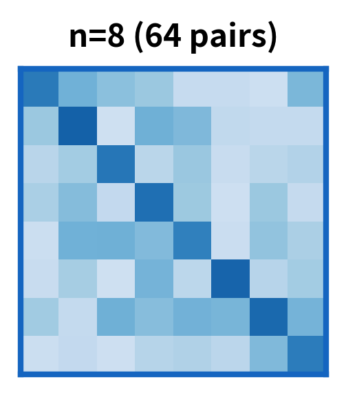
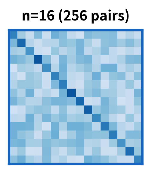
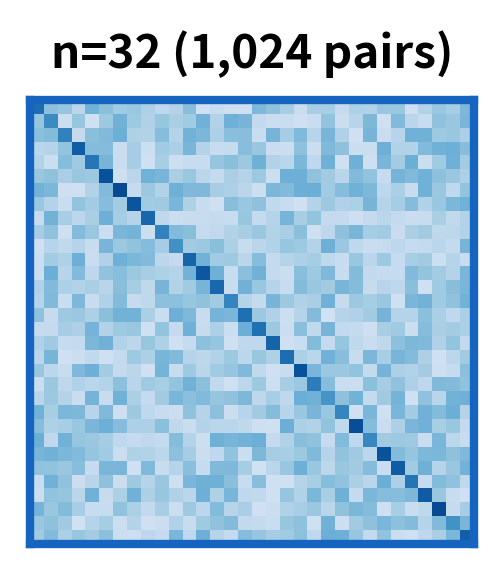
To understand why attention becomes expensive, we need to trace through exactly what happens when self-attention processes a sequence. The mechanism is elegant but computationally demanding, and the cost comes from a single, fundamental fact: every token must interact with every other token.

Imagine you're in a room with $n$ people, and everyone needs to have a brief conversation with everyone else. With 10 people, that's $10 \times 10 = 100$ conversations. With 100 people, it's $100 \times 100 = 10,000$ conversations. The number of interactions grows as the square of the group size. Self-attention faces exactly this scaling challenge.

Self-attention proceeds through three distinct operations, each contributing to the overall computational cost:

1. Computing attention scores: Each token asks "how relevant is every other token to me?" This requires comparing all $n$ tokens against all $n$ tokens.

2. Applying softmax: The raw scores are converted into proper attention weights that sum to 1, allowing us to interpret them as a probability distribution.

3. Computing outputs: Each token gathers information from all other tokens, weighted by the attention scores, to produce its contextual representation.

The first and third steps are where the quadratic cost emerges. Let's examine each one carefully.

The heart of self-attention is measuring pairwise relevance between tokens. Given a sequence of $n$ tokens, we need to compute how strongly each token should attend to every other token. This is done by comparing query vectors against key vectors using the dot product.

Mathematically, we arrange all queries into a matrix $Q$ and all keys into a matrix $K$, then compute:

where:

• $S$: the $n \times n$ attention score matrix, where $S_{ij}$ measures how much token $i$ should attend to token $j$
• $Q$: the query matrix with shape $n \times d_k$, containing one query vector per token
• $K^T$: the transposed key matrix with shape $d_k \times n$, rearranging the key vectors for efficient matrix multiplication
• $n$: the sequence length (number of tokens)
• $d_k$: the dimension of each query/key vector (typically 64 in standard transformers)

Why does this produce $n^2$ values? Each row of $Q$ (one token's query) gets multiplied against every column of $K^T$ (every token's key), producing one score per pair. With $n$ rows and $n$ columns, we get an $n \times n$ grid of scores.

The computational cost of this matrix multiplication is substantial. Each entry in the output matrix requires $d_k$ multiplications and $d_k - 1$ additions. With $n^2$ entries, the total operation count is $n^2 \cdot d_k$.

The critical observation is that this score computation already scales as $O(n^2 d_k)$. The $n^2$ term is unavoidable: we cannot know which token pairs are important without examining all of them.

Raw dot products can be any real number, positive or negative, with no upper bound. To use them as weights for a weighted average, we need to transform them into a valid probability distribution. The softmax function accomplishes this for each row of the score matrix:

For each token $i$, softmax converts its $n$ raw scores into $n$ attention weights that sum to 1. This involves:

1. Computing $\exp(S_{ij})$ for each of the $n$ scores (making them all positive)
2. Summing these exponentials across the row
3. Dividing each exponential by the sum

Each row requires approximately $3n$ operations (exponentiate, sum, divide), and with $n$ rows, the total is $O(n^2)$. While still quadratic, this is dominated by the $O(n^2 d_k)$ cost of score computation when $d_k$ is large.

The final step uses the attention weights to compute a weighted combination of value vectors. Each token's output is a blend of all tokens' values, weighted by attention:

where:

• $\text{softmax}(S)$: the $n \times n$ attention weight matrix, with each row summing to 1
• $V$: the value matrix with shape $n \times d_v$, containing one value vector per token
• $d_v$: the dimension of each value vector (typically equal to $d_k$)

This is another matrix multiplication: $(n \times n) \cdot (n \times d_v)$ produces an $n \times d_v$ output. Each of the $n \cdot d_v$ output elements requires $n$ multiply-accumulate operations (summing across the $n$ positions), giving $n^2 \cdot d_v$ total operations.

This step is just as expensive as score computation. We've now encountered two $O(n^2)$ matrix multiplications.

Summing the costs from all three stages:

where:

• $n$: sequence length
• $d_k$: query/key dimension
• $d_v$: value dimension
• $d$: model dimension (typically $d_k = d_v = d/h$ for $h$ attention heads)

The simplification to $O(n^2 d)$ reflects that $d_k$ and $d_v$ are both proportional to the model dimension $d$. In standard transformers, each head operates on $d/h$ dimensions, but since we have $h$ heads processing in parallel and concatenating their outputs, the total complexity across all heads scales with the full model dimension.

This analysis reveals the fundamental scaling behavior of self-attention:

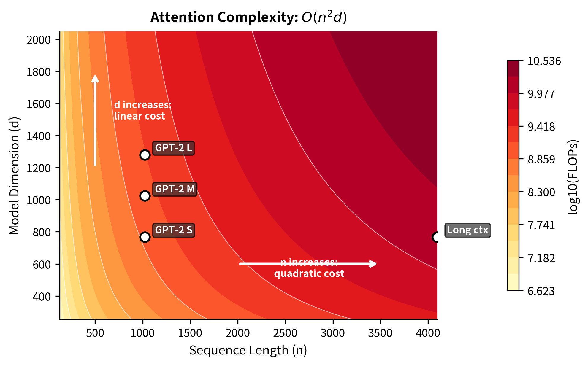
• Quadratic in sequence length: Doubling $n$ quadruples the computation. This is the defining characteristic that limits context length.
• Linear in model dimension: Doubling $d$ only doubles the computation. Making models wider is relatively cheap.

The quadratic term dominates for long sequences. At $n = 1000$ tokens with $d = 768$ (GPT-2 dimensions), the $n^2 = 1,000,000$ factor far exceeds the $d = 768$ factor. Understanding this asymmetry is crucial for reasoning about transformer scalability.

Let's translate this analysis into code. We'll build a function that calculates the exact number of floating-point operations for self-attention, making the complexity formula concrete and verifiable.

The function mirrors our three-stage analysis: score computation contributes $n^2 \cdot d$ operations, softmax contributes $3 \cdot n^2$ operations, and output computation contributes another $n^2 \cdot d$ operations.

With this function, we can explore how computational cost scales across different sequence lengths. We'll use GPT-2's model dimension ($d = 768$) to ground our analysis in real-world numbers.

The table shows the quadratic explosion in computational cost. At sequence length 128, attention requires roughly 25 million operations. By 1024 tokens (a typical context window), we're performing over 1.6 billion operations. At 8192 tokens, this jumps to nearly 100 billion operations. These numbers are per layer only, so a 12-layer transformer multiplies each value by 12.

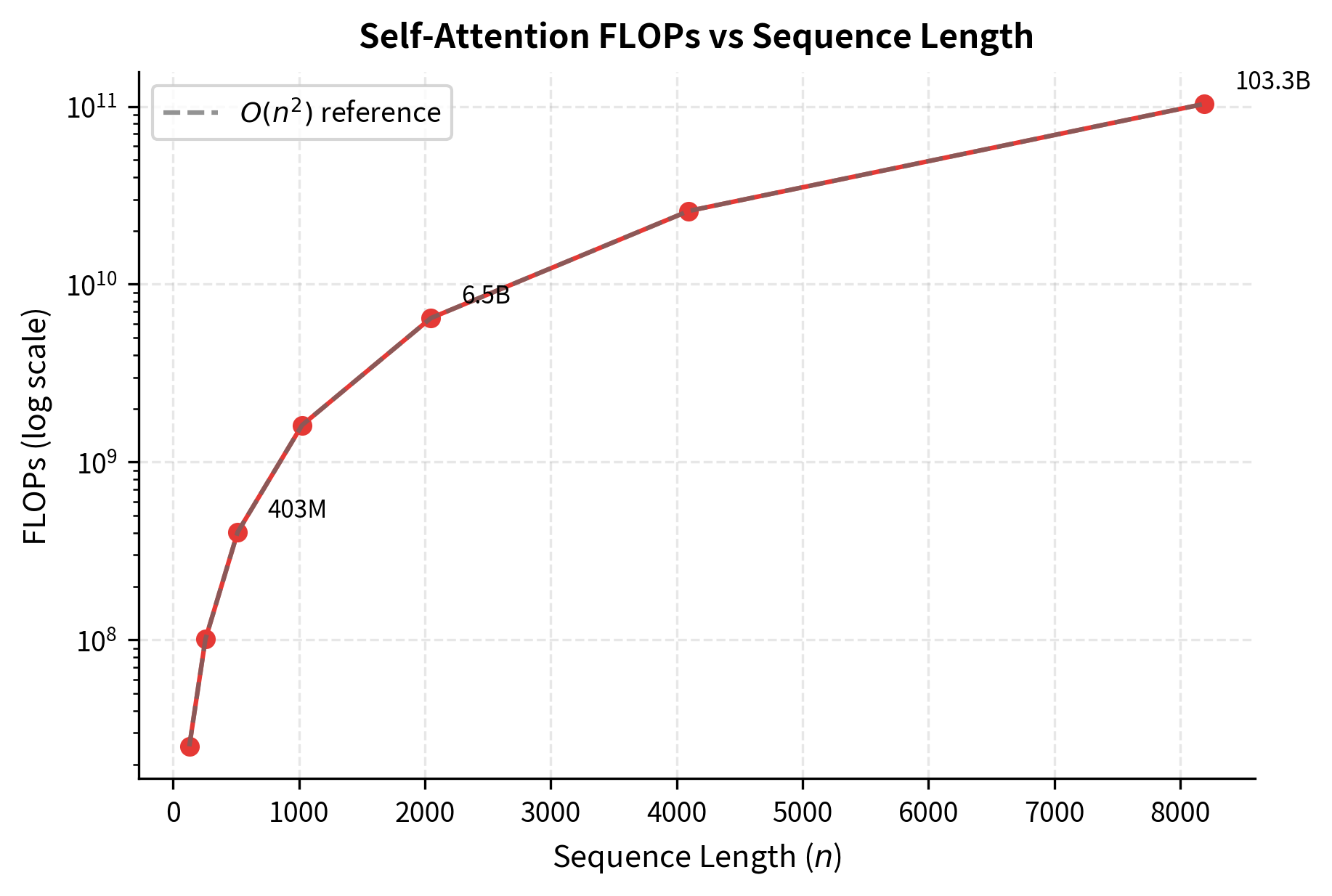
The plot confirms the quadratic relationship. Moving from 512 to 1024 tokens quadruples the computation, and moving from 1024 to 2048 quadruples it again. At the right edge of the plot, we're computing nearly 100 billion operations for a single attention layer.

Computation is only half the story. Memory consumption often becomes the limiting factor before compute does. Self-attention requires storing several large tensors.

The attention weight matrix has shape $n \times n$, where $n$ is the sequence length. For a single attention head, this matrix contains $n^2$ elements. With $h$ heads, we store $h \cdot n^2$ values. Using 32-bit floats (4 bytes each), the memory requirement is:

where:

• $M_{\text{attn}}$: memory required for attention matrices
• $h$: number of attention heads
• $n$: sequence length
• $4$: bytes per element for 32-bit floats (fp32)

For 16-bit floats (common in modern training with fp16 or bf16), this halves to $2 \cdot h \cdot n^2$ bytes. The quadratic dependence on $n$ means that doubling the sequence length quadruples the memory requirement.

A complete forward pass through attention requires storing:

• Query, Key, Value matrices: Each is $n \times d$, totaling $3nd$ elements
• Attention scores/weights: $n^2$ per head, $hn^2$ total
• Output before projection: $n \times d$ elements
• Intermediate activations for backpropagation: Often requires keeping the attention matrix and pre-softmax scores

During training, gradient computation doubles many of these requirements.

The memory requirements reveal the quadratic scaling in action. For GPT-2 Small, moving from 512 to 2048 tokens increases memory by roughly 16x (from ~0.2GB to ~3GB). At 8192 tokens, even the smaller model requires substantial memory. For GPT-2 Medium with its additional layers and heads, the numbers are even larger. These estimates cover only attention matrices and exclude model weights, optimizer states, and gradient storage needed during training.

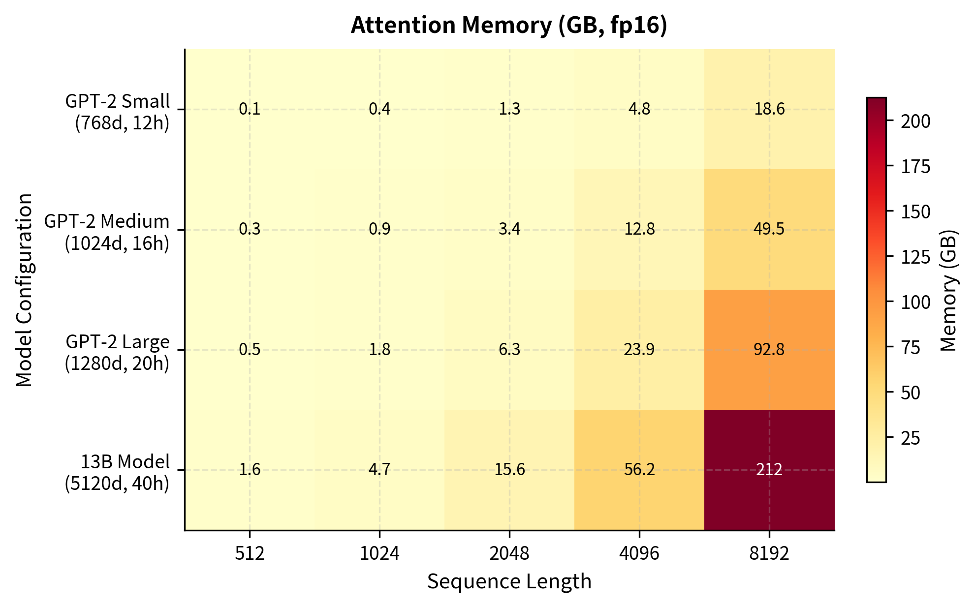
The heatmap reveals a crucial insight: memory grows quadratically with sequence length but only linearly with model size. Doubling from 2048 to 4096 tokens has a larger impact than moving from GPT-2 Small to GPT-2 Large. For truly long sequences, even small models hit memory limits.

To appreciate why the quadratic cost matters, let's compare attention to recurrent neural networks. Both architectures process sequences, but their computational patterns differ fundamentally.

An RNN with hidden dimension $d$ processes each of $n$ tokens sequentially. At each timestep $t$, the hidden state update follows:

where:

• $h_t$: hidden state at timestep $t$ (dimension $d$)
• $W_h$: hidden-to-hidden weight matrix (shape $d \times d$)
• $h_{t-1}$: previous hidden state (dimension $d$)
• $W_x$: input-to-hidden weight matrix (shape $d \times d$, assuming input dimension matches $d$)
• $x_t$: input at timestep $t$
• $\sigma$: activation function (e.g., tanh)

The computational cost per timestep is:

• Matrix-vector multiplication $W_h h_{t-1}$: $O(d^2)$ operations
• Matrix-vector multiplication $W_x x_t$: $O(d^2)$ operations
• Activation function: $O(d)$ operations

Total per step: $O(d^2)$. For $n$ tokens: $O(nd^2)$.

RNN complexity is linear in sequence length and quadratic in hidden dimension.

Summarizing the complexity of each architecture:

• Attention: $O(n^2 d)$
• RNN: $O(nd^2)$

where $n$ is sequence length and $d$ is the hidden/model dimension.

To find when these costs are equal, we set $n^2 d = nd^2$ and solve for $n$:

Dividing both sides by $nd$ (assuming $n, d > 0$):

This crossover point has a clear interpretation: when sequence length exceeds model dimension ($n > d$), attention becomes more expensive. When model dimension exceeds sequence length ($n < d$), RNN becomes more expensive.

The ratio column reveals the crossover behavior. At $n = 64$ and $n = 128$, attention is actually 0.13x and 0.25x the cost of an RNN, respectively, making attention the more efficient choice. At $n = 512$ (exactly equal to $d$), both architectures have identical cost (1.00x ratio). Beyond this point, attention becomes increasingly expensive: at $n = 4096$, attention requires 8x more operations than an equivalent RNN.

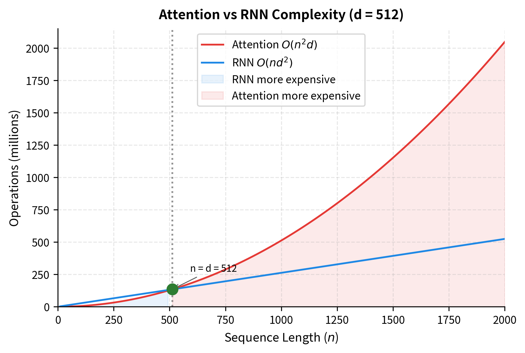
The crossover behavior has practical implications. For short sequences (a few hundred tokens), attention's overhead is minimal. For long documents, books, or conversation histories spanning thousands of tokens, the quadratic cost becomes the dominant bottleneck.

Why use attention despite its higher cost? The answer lies in path length. In an RNN, information from token $i$ to token $j$ must traverse $|j - i|$ sequential steps. In attention, any two tokens connect in a single step.

The "Efficiency" column (path improvement divided by compute ratio) quantifies the value proposition of attention. At $n = 128$, we pay only 0.25x the compute of an RNN while gaining 63x shorter average paths, yielding an efficiency of 252. At $n = 512$ (the crossover point), we pay 1x compute for 255x path improvement. At $n = 2048$, we pay 4x more compute but get 1023x shorter paths. Notice that efficiency remains nearly constant around $d/2 = 256$. This reveals an important insight: as sequence length grows, both the path improvement and the compute penalty scale proportionally with $n$. Attention's value proposition stays roughly constant regardless of sequence length. The short path lengths are always worth the extra compute.

Given the quadratic complexity, what are the practical limits for attention-based models? The answer depends on hardware constraints, training budget, and inference requirements.

Modern GPUs have 16GB to 80GB of memory. With fp16 precision (2 bytes per element), the attention matrix for a single layer with 12 heads at sequence length 8192 requires:

where:

• $M$: memory in bytes
• $h = 12$: number of attention heads
• $n = 8192$: sequence length
• $b = 2$: bytes per element (fp16)

For a 12-layer model, that's approximately 18GB just for attention matrices, before accounting for model weights, other activations, or gradients. Training requires additional memory for optimizer states (often 2x the model size for Adam) and gradient accumulation.

These estimates assume 70% of GPU memory is available for attention matrices (the remaining 30% accounts for model weights and other overhead). An RTX 3090 with 24GB can handle approximately 27K tokens, while an A100 80GB extends this to around 50K tokens. These numbers represent theoretical upper bounds for a single sample with batch size 1. In practice, larger batch sizes for training efficiency, gradient storage for backpropagation, and optimizer states further reduce these limits. Production systems address these constraints through gradient checkpointing, FlashAttention, and model parallelism.

Beyond memory, compute time imposes practical limits. Processing long sequences is slow.

At 512 tokens, attention completes in a fraction of a millisecond. By 4096 tokens, latency grows but remains acceptable for most applications. At 32K tokens, attention alone approaches double-digit milliseconds per forward pass. The "Tokens/sec" column shows throughput in terms of context size processed: higher values indicate more efficient processing for that context length. During training with backpropagation, multiply these times by roughly 3x. For autoregressive generation where the full context is reprocessed for each new token, long contexts compound these costs significantly.

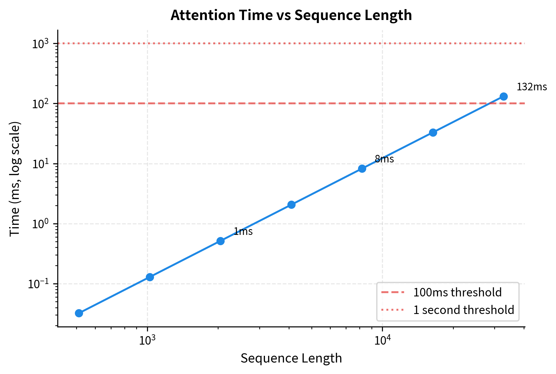
The timing curve shows why context length is such a hot topic in LLM development. Crossing the 100ms threshold makes interactive applications sluggish. Crossing 1 second makes them impractical for real-time use.

The combination of quadratic time and space complexity creates what's known as the attention bottleneck. As we push for longer context windows, attention becomes the dominant cost, often exceeding the cost of feed-forward layers, embeddings, and everything else combined.

The percentages reveal how computational burden shifts with sequence length. At 256 tokens, attention accounts for only about 5% of layer computation, with the feed-forward network dominating at around 69%. By 1024 tokens, attention grows to roughly 17%, and at 4096 tokens it reaches approximately 45%, nearly matching the FFN. The projection layers (QKV and output) remain relatively stable since they scale linearly with $n$. This distribution explains why optimizing attention becomes critical for long-context applications while being less important for short sequences.

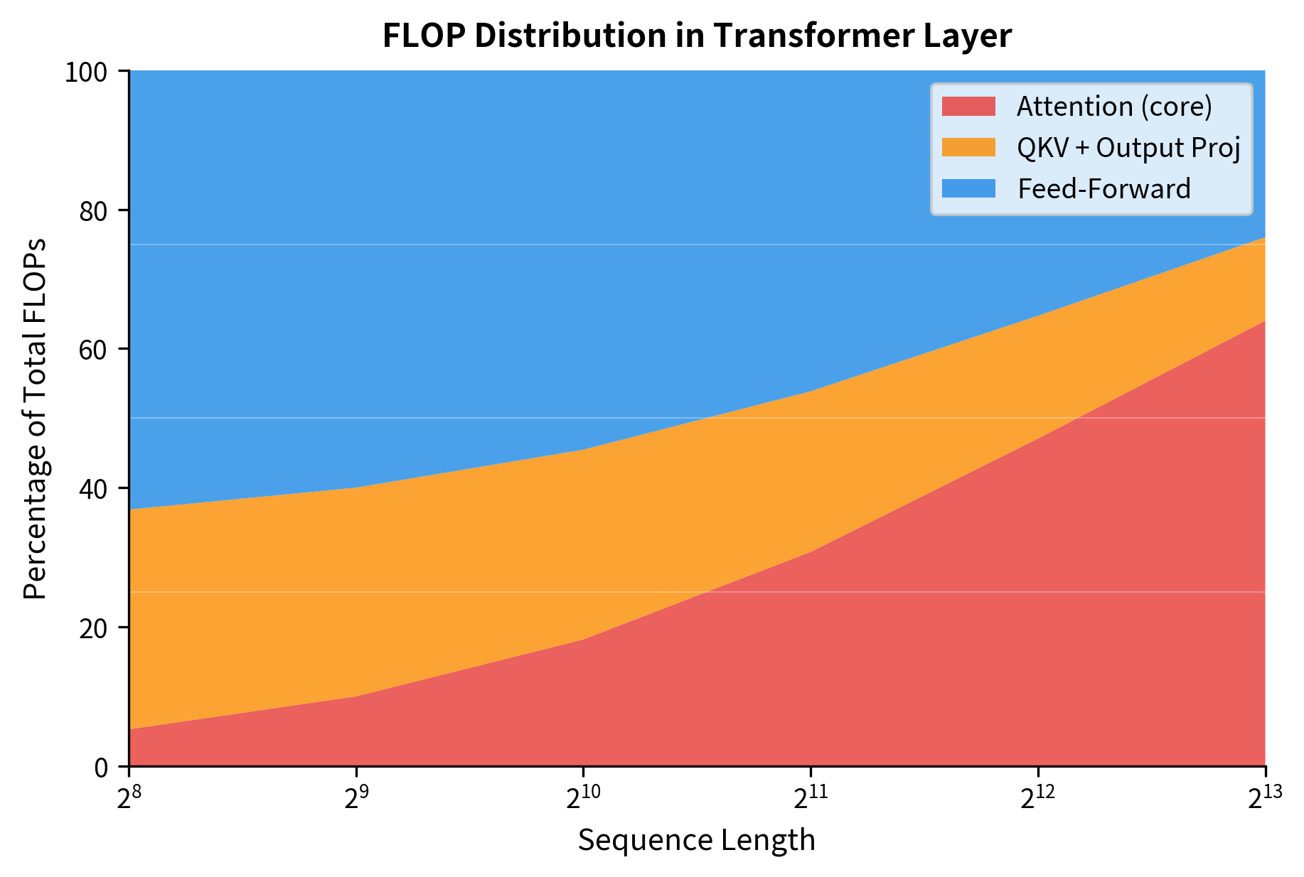
This visualization shows the attention bottleneck in action. The red region (attention core) expands as sequence length grows, squeezing out other components. This is why efficient attention mechanisms are such an active research area.

The quadratic complexity of standard attention has motivated numerous alternatives. While a detailed treatment of each variant deserves its own chapter, understanding the landscape helps contextualize the complexity analysis.

Several methods approximate attention with linear complexity by avoiding the explicit $n \times n$ matrix:

• Linformer: Projects keys and values to lower dimensions before computing attention
• Performer: Uses random feature maps to approximate softmax attention in $O(n)$
• Linear Transformers: Replace softmax with kernel functions that allow associative computation

These methods trade accuracy for speed, often working well in practice despite theoretical approximation.

Instead of attending to all positions, sparse methods attend to a subset:

• Longformer: Combines local windowed attention with global attention on special tokens
• BigBird: Uses a combination of random, window, and global attention patterns
• Sparse Transformers: Learn which positions to attend to

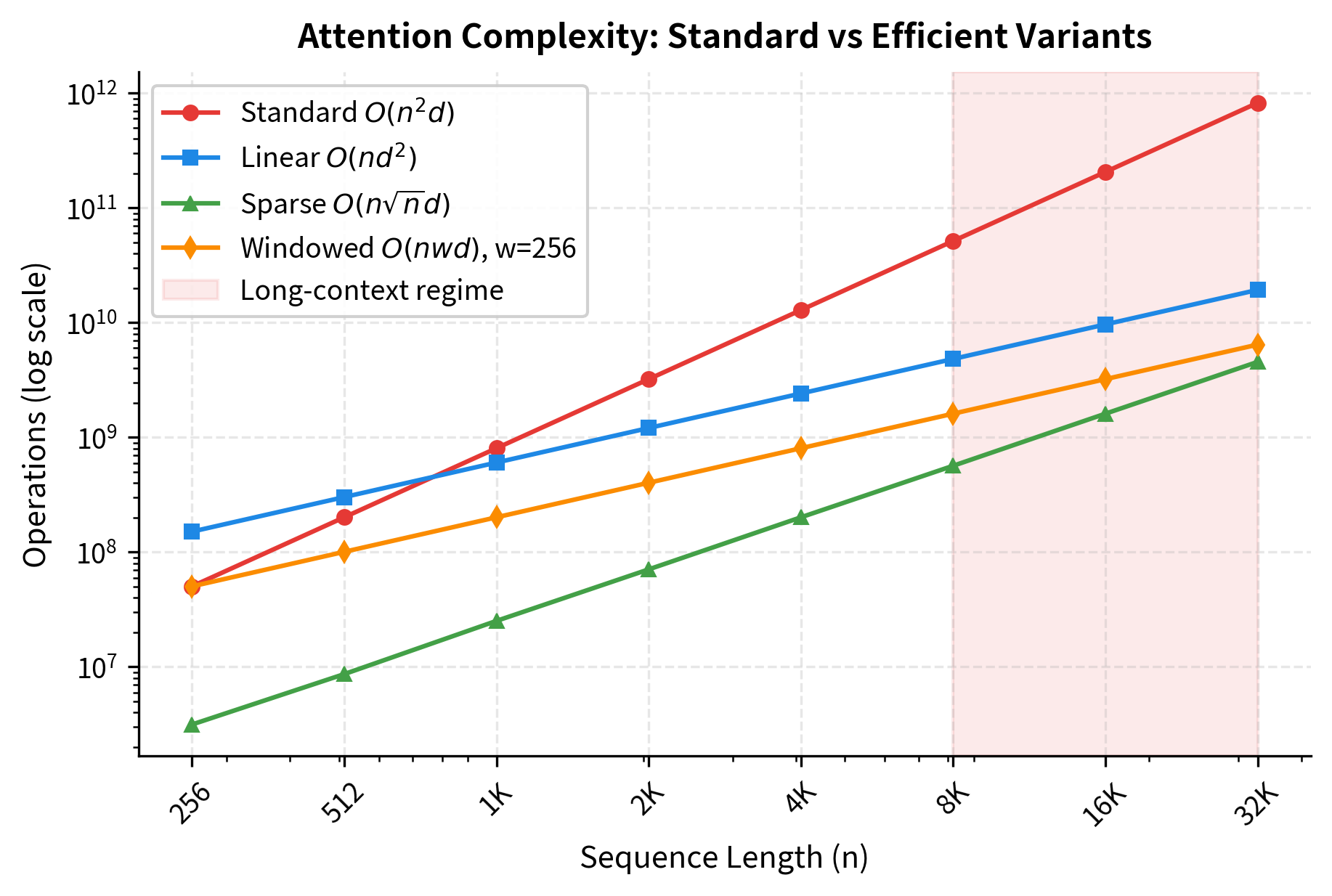
Sparse attention reduces complexity to $O(n \cdot k)$, where:

• $n$: sequence length
• $k$: number of positions each token attends to (typically $k \ll n$)

For example, with a local window of 256 tokens, $k = 256$ regardless of sequence length, making the complexity effectively linear in $n$.

Some methods restructure the computation to reduce memory:

• Flash Attention: Reorders operations to minimize memory transfers, achieving the same result with less memory
• KV Caching: During generation, caches key-value pairs to avoid recomputation
• Gradient Checkpointing: Trades computation for memory by recomputing activations during backward pass

The speedup factors demonstrate why efficient attention variants are essential for long sequences. Standard attention at 16K tokens requires over 200 billion operations. Linear attention, which trades the $n^2$ term for $d^2$, achieves roughly a 21x speedup by avoiding the explicit attention matrix. Sparse attention with $k = \sqrt{n} \approx 128$ positions achieves similar gains. Windowed attention with a fixed 256-token window provides approximately 64x speedup, making it highly effective for tasks where local context dominates. These variants enable practical processing of long documents, book-length texts, and extended conversations that would be prohibitively expensive with standard attention.

The quadratic complexity of attention is both its greatest strength and most significant limitation. The all-pairs computation enables transformers to capture any dependency regardless of distance, but it also creates hard limits on context length that no amount of hardware can fully overcome.

For practitioners, understanding these complexity bounds is essential for making informed architecture decisions. When processing short sequences (a few hundred tokens), attention overhead is negligible compared to feed-forward layers. In this regime, you can use standard attention without concern. However, when context length grows into the thousands or tens of thousands, attention becomes the dominant cost. You need to consider sparse attention variants, linear approximations, or hierarchical processing strategies. The crossover point depends on your model size, but for typical configurations, it occurs around 512-1024 tokens.

Memory constraints often bite before compute constraints do. During training, storing attention matrices for backpropagation requires $O(n^2)$ memory per layer. This quadratic memory scaling is why long-context training requires techniques like gradient checkpointing (trading compute for memory), FlashAttention (reordering operations to reduce memory), or model parallelism (distributing across multiple GPUs). The memory bottleneck also affects inference, especially when serving many concurrent requests with long contexts.

The complexity analysis also explains why efficient attention is such an active research area. Linearizing attention, sparsifying attention patterns, and approximating attention with lower-rank structures are all attempts to break the quadratic barrier while preserving the benefits of all-pairs interaction. These techniques have enabled models with 100K+ token context windows, but they often involve trade-offs in accuracy or increased implementation complexity. Understanding when these trade-offs are acceptable requires understanding the underlying complexity.

Attention's quadratic complexity is a fundamental characteristic that shapes how we design, train, and deploy transformer models. In this chapter, we analyzed this complexity from multiple angles and explored its practical implications.

Key takeaways:

• Time complexity: Standard self-attention requires $O(n^2 d)$ operations, where $n$ is sequence length and $d$ is model dimension. The $n^2$ term means doubling sequence length quadruples computation.

• Memory complexity: Storing attention matrices requires $O(h \cdot n^2)$ memory, where $h$ is the number of heads. This quadratic memory scaling often becomes the limiting factor before compute does.

• Crossover with RNN: Setting $n^2 d = nd^2$ shows that attention is cheaper than RNN when $n < d$, but more expensive when $n > d$. For typical model dimensions (512-4096), attention becomes more expensive beyond a few hundred tokens.

• Practical limits: GPU memory and compute time impose hard constraints on context length. Even with 80GB GPUs, sequence lengths beyond tens of thousands of tokens require specialized techniques.

• The attention bottleneck: As sequence length grows, attention dominates transformer computation, consuming 50% or more of total FLOPs at long contexts.

• Efficient alternatives: Linear attention, sparse attention, and memory-efficient implementations can reduce complexity from $O(n^2)$ to $O(n)$ or $O(n \cdot k)$, where $k$ is the number of attended positions, enabling much longer contexts.

Understanding these complexity characteristics is essential for choosing appropriate architectures, estimating computational requirements, and knowing when to apply optimization techniques. The quadratic wall is real, but it can be navigated with the right tools and understanding.

When analyzing or estimating attention complexity, several parameters directly impact computational and memory requirements:

• n (sequence length): The number of tokens in the input sequence. This is the most critical parameter since complexity scales quadratically with it. Typical values range from 512 to 128K+ in modern models.

• d (model dimension): The embedding dimension of the model. Common values include 768 (GPT-2 Small), 1024 (GPT-2 Medium), 4096 (LLaMA 7B), and larger for bigger models. Complexity scales linearly with this parameter.

• h (number of heads): The number of attention heads. Each head operates on $d/h$ dimensions. More heads mean more parallel attention patterns but also more attention matrices to store.

• L (number of layers): Total transformer layers. Memory and compute scale linearly with layer count, so a 24-layer model requires twice the resources of a 12-layer model.

• dtype_bytes: Precision of floating-point representation. fp32 uses 4 bytes, fp16/bf16 use 2 bytes. Half precision halves memory requirements and often doubles throughput on modern GPUs.

• batch_size: Number of sequences processed simultaneously. Memory scales linearly with batch size, often requiring batch size reduction for long sequences.

Ready to test your understanding? Take this quick quiz to reinforce what you've learned about attention complexity and efficient alternatives.