Encoder Architecture: Bidirectional Transformers for Understanding Tasks

The transformer, introduced in "Attention Is All You Need," combined an encoder and a decoder to handle sequence-to-sequence tasks like machine translation. But a striking realization emerged shortly after: you don't always need both components. For tasks that require understanding rather than generating text, the encoder alone suffices. This insight led to BERT and a family of encoder-only models that dominated NLP benchmarks for years.

Encoder-only transformers process an entire input sequence and produce rich, contextualized representations for each token. Unlike decoders, which generate text one token at a time, encoders see the full context at once. This bidirectional nature makes them ideal for classification, named entity recognition, question answering, and semantic similarity tasks.

This chapter explores the encoder architecture in depth. We'll examine how bidirectional self-attention differs from the causal attention used in decoders, understand why encoders excel at understanding tasks, and implement a complete encoder from scratch. By the end, you'll understand the design principles that made BERT and its descendants so successful.

The original transformer uses both an encoder to process input and a decoder to generate output. For translation, the encoder reads the source sentence while the decoder produces the target sentence token by token. This separation makes sense when input and output differ in length and structure.

But many NLP tasks don't require generation at all. Sentiment analysis asks: is this review positive or negative? Named entity recognition asks: which words are person names, locations, or organizations? Question answering asks: which span in the passage answers this question? These are all understanding tasks. You need to comprehend the input text, not produce new text.

For understanding tasks, an encoder-only architecture offers three key advantages:

1. Bidirectional context: Each token can attend to tokens both before and after it, capturing richer context than left-to-right processing allows.

2. Computational efficiency: Without a decoder, you eliminate cross-attention and the sequential generation loop, making inference faster for classification tasks.

3. Simpler training: You can train on masked language modeling without needing parallel text pairs (source and target sentences).

The encoder produces one representation vector per input token. Depending on the task, you might use the first token's representation for classification, all representations for sequence labeling, or specific span representations for extraction tasks.

The defining feature of encoders is bidirectional self-attention. Every token can attend to every other token in the sequence, including tokens that appear after it. This contrasts sharply with the causal (masked) attention used in decoders, where each token can only attend to previous tokens.

Consider processing the sentence "The bank approved the loan quickly." When computing the representation for "bank," bidirectional attention sees:

• Before: "The"
• After: "approved the loan quickly"

The word "loan" in the future context helps disambiguate that "bank" refers to a financial institution rather than a river bank. Causal attention would miss this crucial signal, seeing only "The" before "bank."

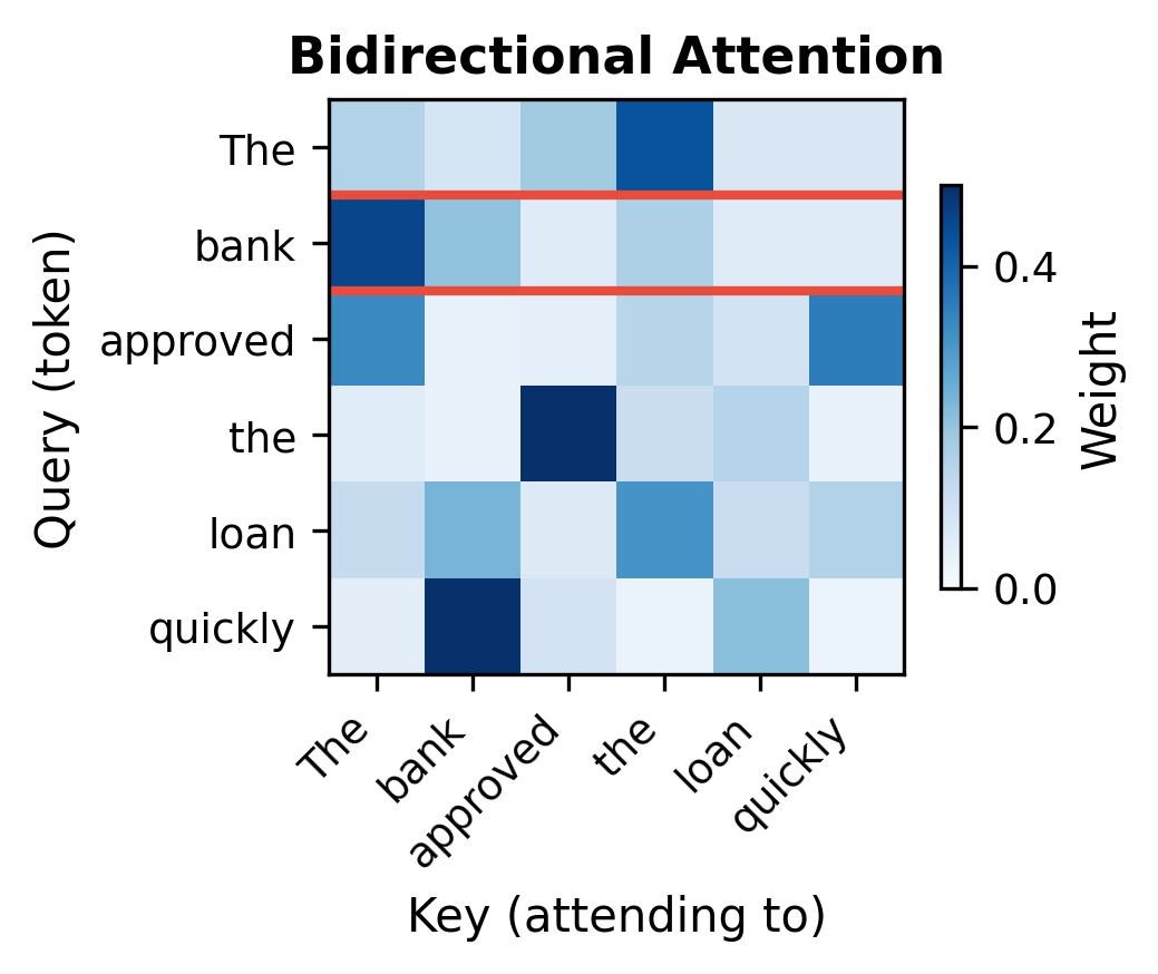
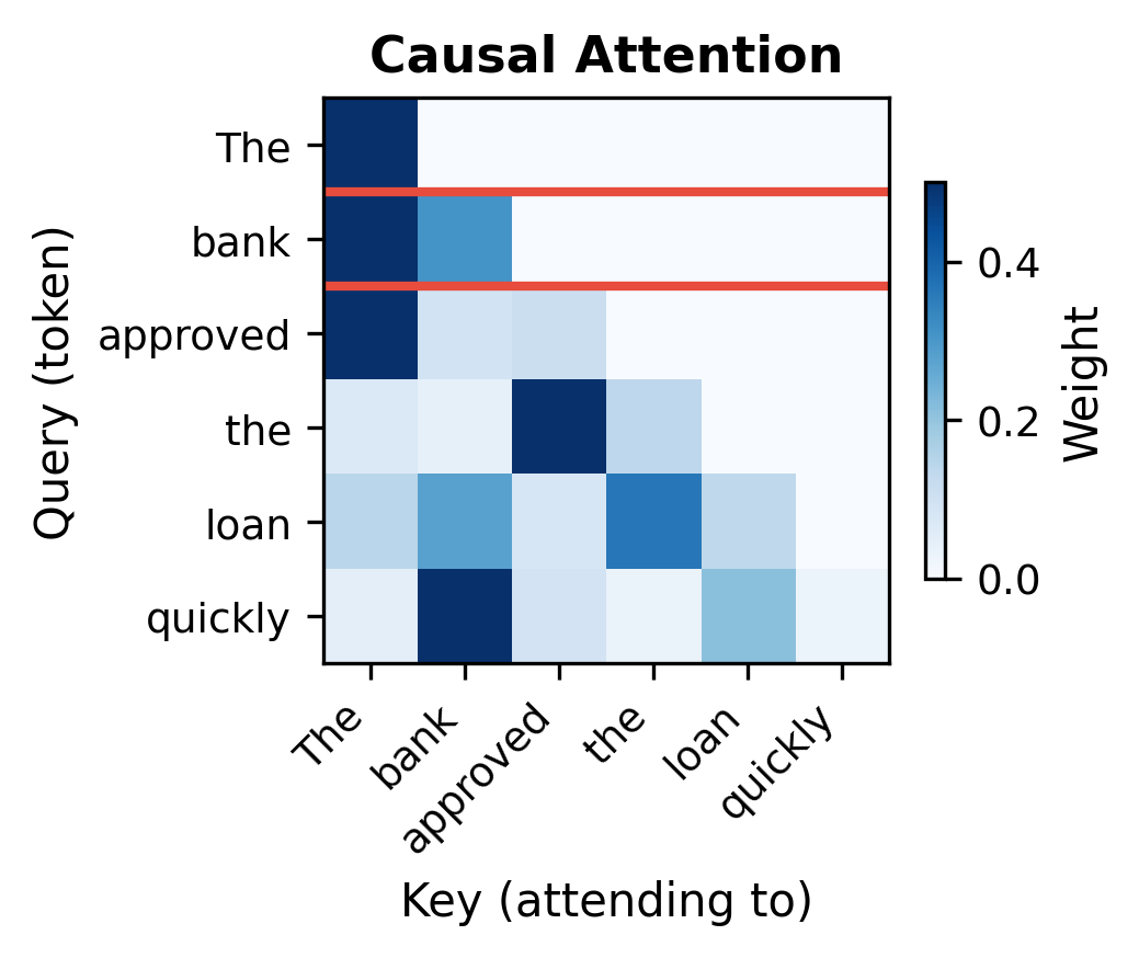
The visualizations reveal the fundamental difference. In bidirectional attention (left), the "bank" row shows non-zero weights for all six positions, including "loan" and "quickly" that appear later in the sequence. In causal attention (right), the "bank" row shows weights only for "The" and "bank" itself. The future context that would help disambiguate "bank" is completely invisible.

To understand how bidirectional attention works mathematically, we need to build up from a simple question: how does a token decide which other tokens to pay attention to?

The answer involves three learned projections that give each token different "roles" in the attention computation. Think of it as a information retrieval system where tokens can both ask questions and provide answers:

1. Queries represent what a token is looking for. When computing the representation for "bank," its query vector encodes the question "what information do I need to understand my meaning?"

2. Keys represent what a token offers. Each token advertises its content through a key vector, saying "this is what I can tell you about."

3. Values contain the actual information to be gathered. Once attention decides which tokens matter, their value vectors provide the content.

Starting from the input sequence $X \in \mathbb{R}^{n \times d}$ containing $n$ tokens with $d$-dimensional embeddings, we project into these three spaces:

where:

• $X$: the input matrix with one row per token
• $W^Q, W^K, W^V \in \mathbb{R}^{d \times d_k}$: learned projection matrices
• $Q, K, V$: the resulting query, key, and value matrices

With these projections in hand, we measure relevance by computing dot products between queries and keys. A high dot product between query $i$ and key $j$ means token $i$ should attend strongly to token $j$. We arrange all these dot products into a single matrix multiplication:

This produces an $n \times n$ matrix where entry $(i, j)$ measures how much token $i$ should attend to token $j$. The key insight for encoders: we compute all $n^2$ entries, not just the lower triangle. Position 2 can attend to position 5, and position 5 can attend to position 2.

Raw dot products can grow large as the dimension $d_k$ increases, which would push softmax into regions with vanishing gradients. To stabilize training, we scale by $\sqrt{d_k}$:

The softmax function converts these scores into a probability distribution. For each token (each row), softmax ensures the attention weights across all positions sum to 1:

Finally, we use these weights to compute a weighted average of value vectors. If token $i$ assigns weight 0.4 to token $j$, then 40% of $j$'s value vector contributes to $i$'s output:

Putting it all together, the complete attention formula is:

where:

• $Q = XW^Q$: query matrix, each row is a token asking "what should I pay attention to?"
• $K = XW^K$: key matrix, each row is a token advertising "this is what I contain"
• $V = XW^V$: value matrix, each row is a token's actual content to be gathered
• $d_k$: dimension of query/key vectors, used for scaling to prevent gradient issues
• The softmax normalizes attention weights to sum to 1 for each query position

The crucial difference from decoder attention: no mask is applied before the softmax. Every query-key pair contributes to the attention weights, allowing information to flow in both directions. This is the simplest form of self-attention, with no architectural constraints on which positions can interact.

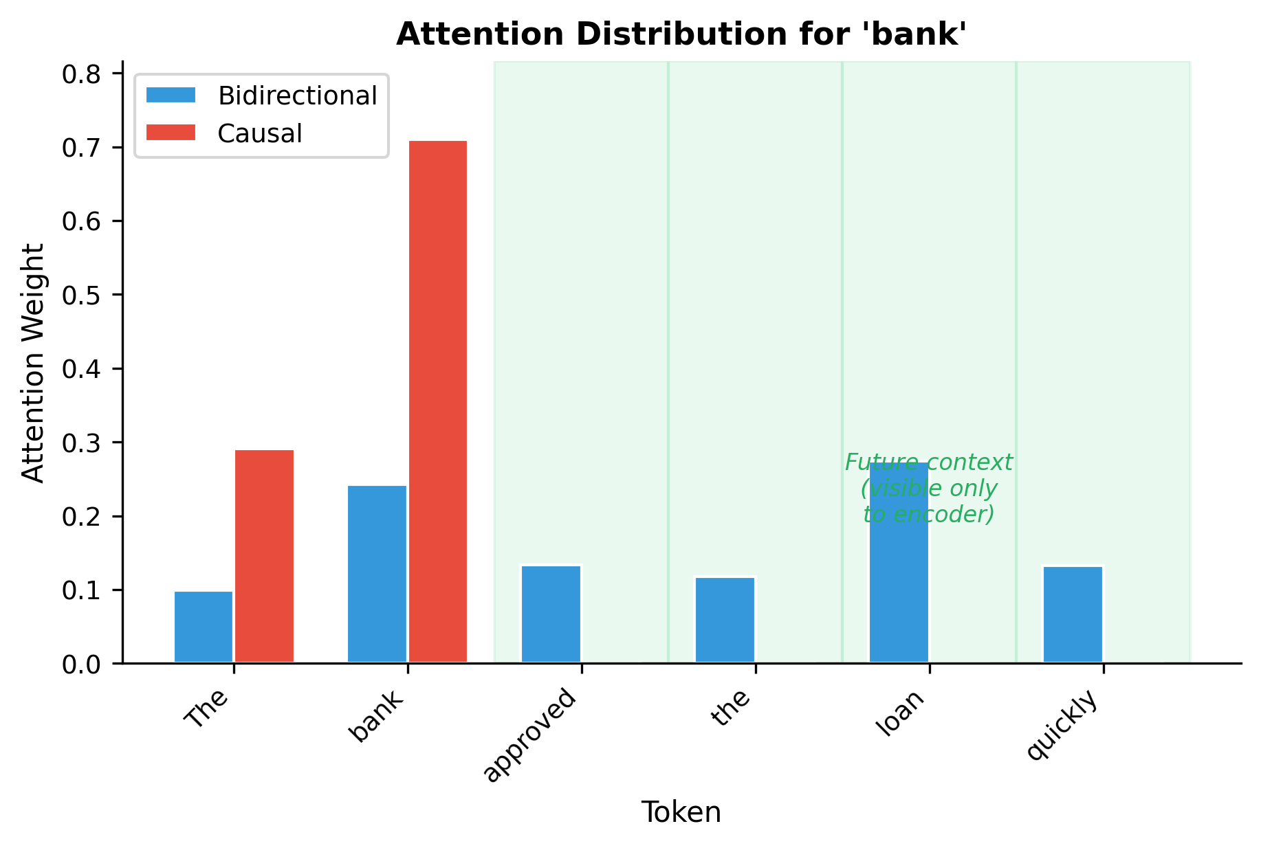
The visualization quantifies what bidirectional attention enables. With bidirectional attention, "bank" draws information from all tokens, including future tokens like "loan" and "quickly" that appear later in the sequence. With causal attention, these future tokens contribute zero weight. The representation of "bank" differs fundamentally depending on which attention pattern is used.

Bidirectional attention makes encoders powerful tools for tasks that require comprehending input text. Let's examine the major categories of tasks where encoder-only models excel.

Classification maps an entire input sequence to a single label: sentiment (positive/negative), topic (sports/politics/technology), or intent (question/command/statement). The encoder processes the full sequence, then a classification head converts the representation to class probabilities.

Why use [CLS] rather than averaging all token representations? The [CLS] token starts with no inherent meaning. Through self-attention, it learns to collect task-relevant information from the actual content tokens. This learned aggregation often outperforms simple averaging, especially for tasks requiring holistic understanding.

Named entity recognition, part-of-speech tagging, and similar tasks require a label for each token, not just one label for the whole sequence. Here, every token's encoder representation passes through a classification head:

Each token gets its own contextualized representation that incorporates information from the entire sentence. When classifying "Google," the encoder representation already knows that "John works at" precedes it and "in California" follows it, helping distinguish company names from other uses of the word.

Given a question and a passage, extractive QA identifies the span in the passage that answers the question. The encoder processes the concatenated question and passage, then two classification heads predict the start and end positions of the answer span:

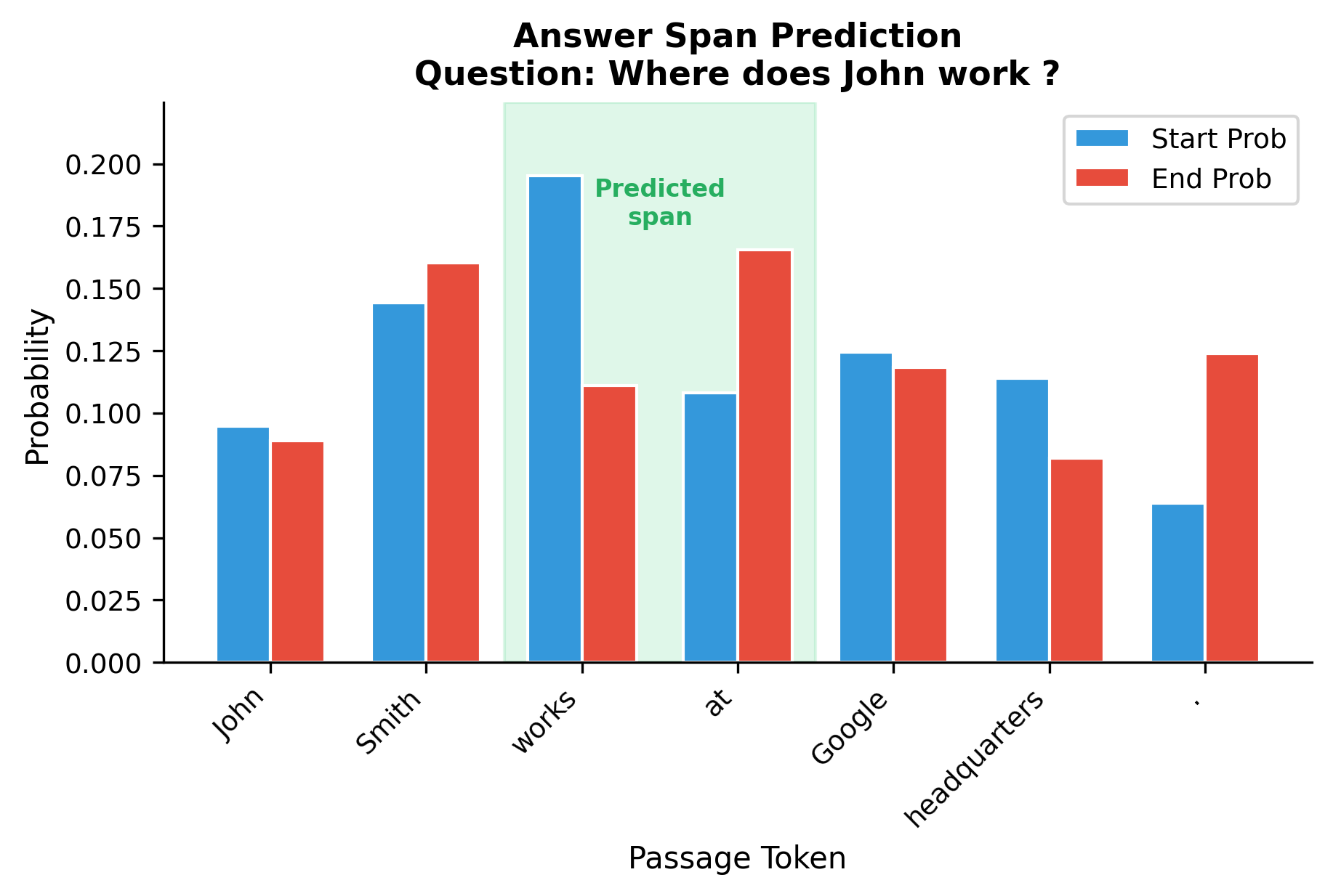
The bidirectional nature is crucial here. When evaluating whether "Google" is the answer, the model simultaneously considers the question "Where does John work?" and the surrounding context "works at ... headquarters." This holistic view is only possible with bidirectional attention.

Having understood the attention mechanism, we can now assemble a complete encoder layer. But attention alone isn't enough. Deep networks need architectural support to train successfully, and encoder layers combine several components that work together to enable learning.

An encoder layer has two major sublayers, each solving a different problem:

1. Multi-head self-attention enables tokens to gather information from each other. This is where bidirectional context mixing happens.

2. Feed-forward network (FFN) processes each token independently through a nonlinear transformation. This adds capacity that pure attention lacks.

Both sublayers are wrapped with two additional mechanisms that make deep stacking possible:

• Residual connections add the input directly to the output of each sublayer. This creates "gradient highways" that allow learning signals to flow through many layers without vanishing.

• Layer normalization stabilizes the distribution of activations, preventing them from exploding or collapsing as they pass through many transformations.

The modern pre-norm configuration places normalization before each sublayer rather than after. This ordering provides cleaner gradient flow and has become the standard for deep transformers. The complete computation unfolds in two stages:

Stage 1: Attention sublayer

First, we normalize the input $\mathbf{x}$. Then attention computes context-aware representations. Finally, we add the original input back (the residual connection). The result $\mathbf{h}$ blends the original representation with information gathered from other positions.

Stage 2: Feed-forward sublayer

The same pattern repeats: normalize, transform, add residual. The FFN applies the same transformation independently to each token position, adding nonlinearity and additional learnable capacity.

Together, these stages form the encoder layer's output:

where:

• $\mathbf{x} \in \mathbb{R}^{n \times d}$: input to the encoder layer, containing $n$ token representations
• $\text{LayerNorm}(\cdot)$: normalizes activations to have zero mean and unit variance per token
• $\text{MultiHeadAttention}(\cdot)$: bidirectional multi-head self-attention (no causal mask)
• $\text{FFN}(\cdot)$: position-wise feed-forward network with nonlinear activation
• $\mathbf{h}$: intermediate representation after the attention sublayer
• $\mathbf{y}$: final output of the encoder layer, same shape as input

Notice that the output $\mathbf{y}$ has the same shape as the input $\mathbf{x}$. This dimensional consistency is what allows us to stack encoder layers: the output of one layer becomes the input to the next, with each layer progressively refining the representations.

Let's implement each component, starting with the building blocks:

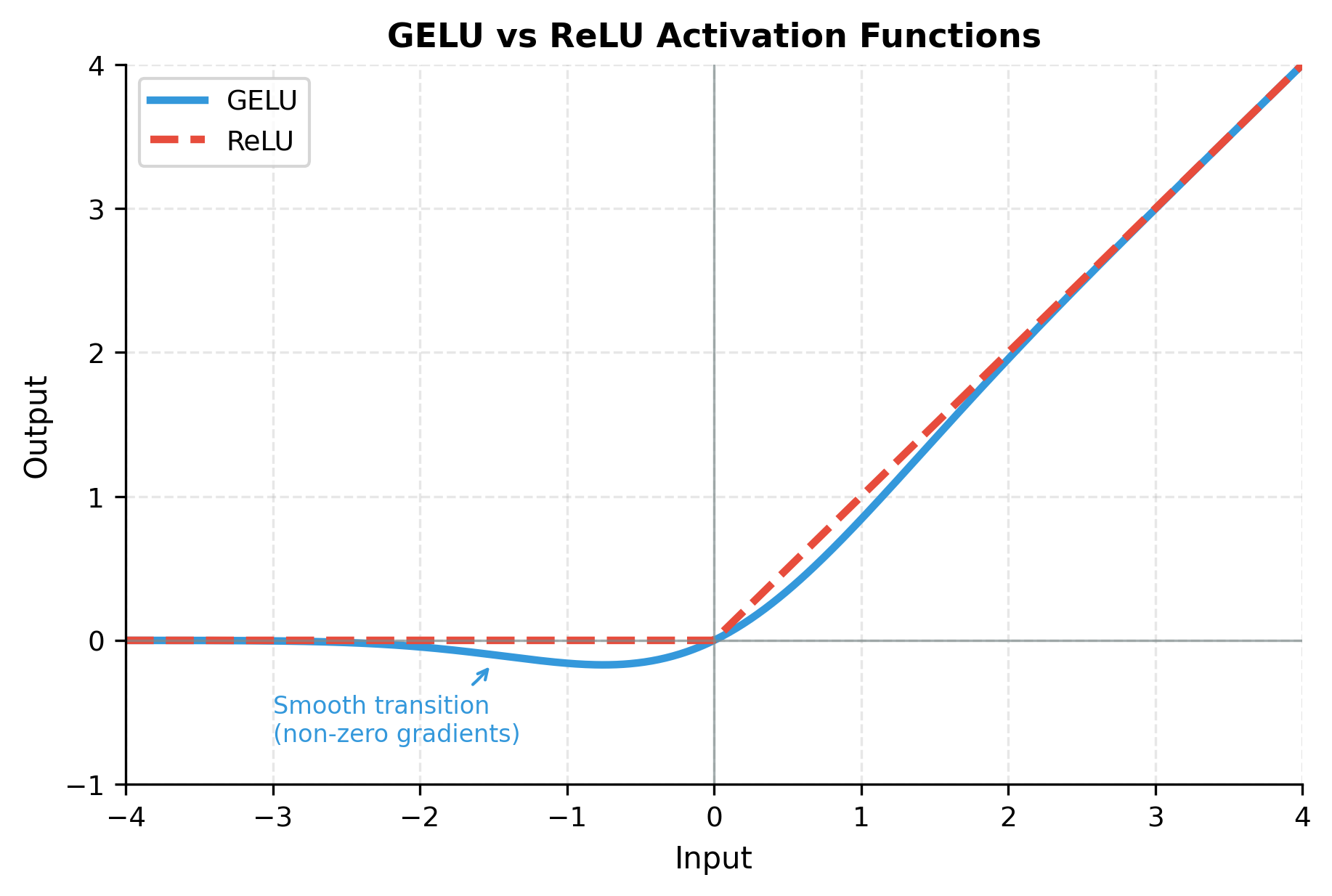
The feed-forward network uses GELU (Gaussian Error Linear Unit) activation, which has become the standard for transformer models. Unlike ReLU which hard-thresholds at zero, GELU provides smooth gating that depends on the input's magnitude:

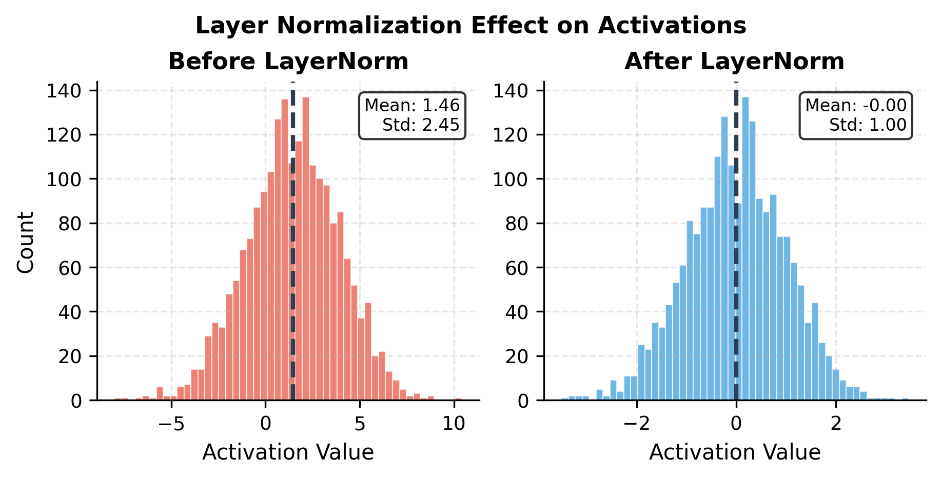
Let's visualize how layer normalization transforms the activation distributions:

Now we assemble these components into a complete encoder layer:

The encoder layer preserves the input shape: a sequence of $n$ tokens with $d$-dimensional representations goes in, and an identically shaped sequence comes out. The attention weights have shape (n_heads, seq_len, seq_len), showing that each head computes its own full attention matrix over all position pairs.

Different attention heads learn to focus on different aspects of the input. Some might attend to adjacent tokens (capturing local syntax), while others span long distances (capturing semantic relationships). Let's visualize how the 8 attention heads in our encoder layer distribute their attention differently:

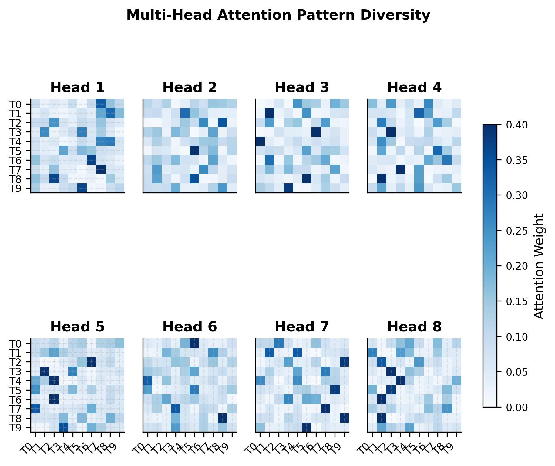
The variation across heads illustrates why multi-head attention is so powerful. No single head needs to capture all relationships. The ensemble of heads provides coverage across local patterns, position-specific attention, and long-range dependencies. During training, each head specializes for patterns that help the overall task.

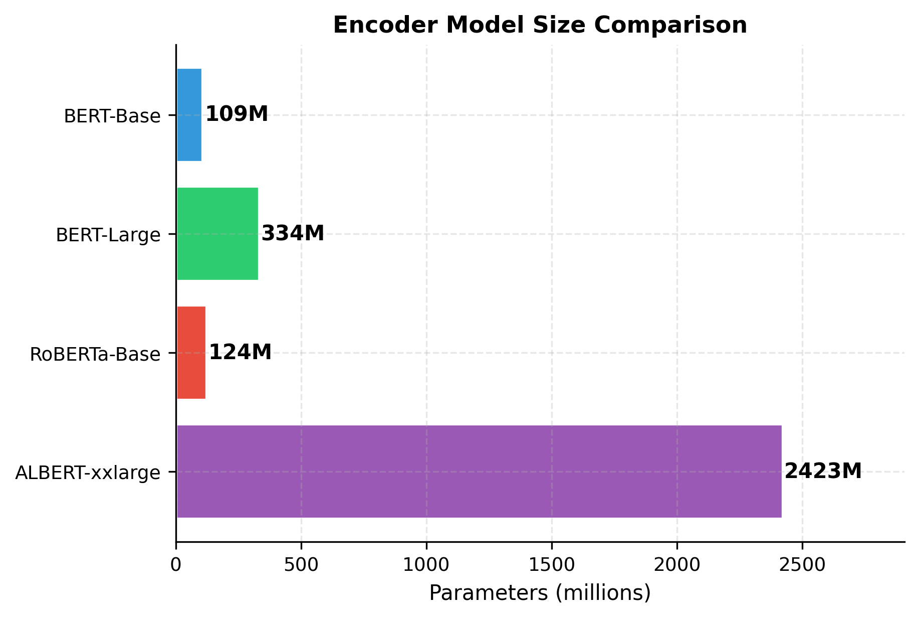
A single encoder layer provides limited representational power. Real models stack many layers, allowing each successive layer to refine the representations further. BERT-Base uses 12 layers, BERT-Large uses 24, and some models go even deeper.

Let's visualize how representations evolve through the layers:

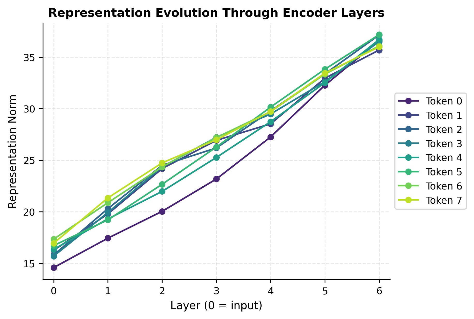
The visualization shows how representations develop across layers. Early layers might have more variable norms as they begin processing the input, while deeper layers tend to stabilize as the residual connections accumulate refined representations.

A useful diagnostic for understanding encoder behavior is attention entropy, a measure of how concentrated or diffuse each token's attention is. High entropy means attention is spread broadly; low entropy means it focuses on specific positions.

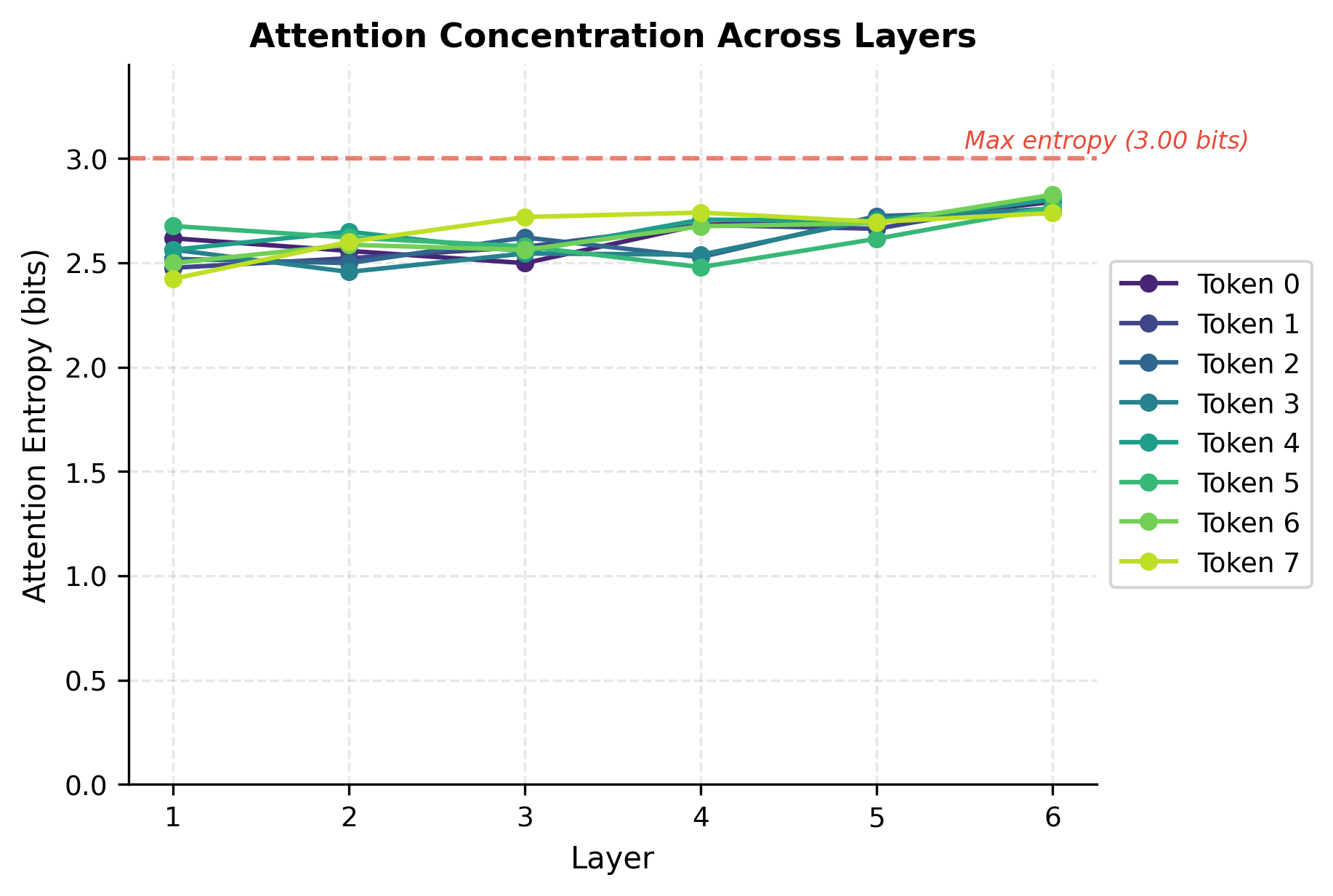
Entropy close to the maximum (dotted line) indicates uniform attention, meaning every token attends roughly equally to all positions. Lower entropy indicates more selective attention. Tracking entropy across layers reveals how the encoder progressively refines its attention patterns from broad context gathering to more task-specific focus.

The encoder produces one contextualized representation per input token. How you use these representations depends on your downstream task.

For classification, sentiment analysis, or any task requiring a single output for the whole sequence, use the [CLS] token representation:

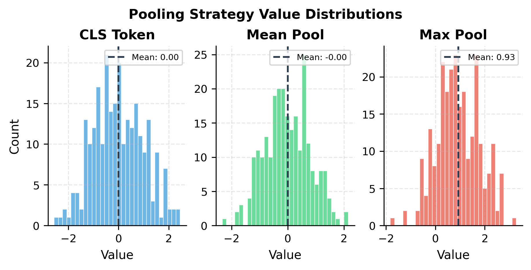
Mean pooling often works well when all tokens contribute equally (like sentence similarity). CLS pooling is preferred when the model was pre-trained to aggregate into the first position. Max pooling can capture salient features but may be sensitive to outliers.

For NER, POS tagging, or other sequence labeling tasks, use every token's representation:

For question answering, relation extraction, or any task involving text spans, you might need to construct span representations from multiple tokens:

BERT established conventions that influenced nearly all subsequent encoder models. Let's examine the specific architectural choices that defined BERT and its variants.

Several architectural choices recur across encoder models.

Head dimension: BERT maintains 64 dimensions per attention head, computed as:

where:

• $d_k$: the dimension of each attention head's query and key vectors
• $d_{\text{model}}$: the model's hidden dimension (768 for BERT-Base)
• $n_{\text{heads}}$: the number of parallel attention heads (12 for BERT-Base)

This gives $d_k = 768 / 12 = 64$ for BERT-Base. The choice balances expressiveness per head with having multiple heads for diverse attention patterns.

FFN expansion: The feed-forward network uses a 4x expansion factor. With $d_{\text{model}} = 768$, the FFN hidden dimension is $768 \times 4 = 3072$. This ratio has become a standard convention, providing a computational "bottleneck" where most of the model's parameters reside.

Vocabulary and positions: BERT uses WordPiece tokenization with a 30K vocabulary and supports sequences up to 512 tokens. Later models like RoBERTa expand the vocabulary and some variants extend to longer sequences.

Let's bring everything together into a complete, production-style encoder implementation:

Encoder-only models have proven remarkably effective for understanding tasks, but they come with inherent limitations that inform when to use them and when to consider alternatives.

The most fundamental limitation is that encoders cannot generate text. They produce representations, not sequences. For tasks like translation, summarization, or dialogue, you need a decoder or encoder-decoder architecture. Attempting to force an encoder to generate by iteratively predicting tokens is inefficient and poorly suited to the architecture's design.

This limitation shapes the NLP landscape. BERT excels at classification, extraction, and similarity tasks, but GPT and its descendants dominate text generation. Understanding which architecture fits your task is crucial.

The bidirectional nature that makes encoders powerful also constrains how they can be trained. You cannot simply predict the next token because the model can already see it. BERT's masked language modeling (MLM) objective works around this by hiding some tokens and predicting them, but this introduces a train-test mismatch: during training, the model sees [MASK] tokens that never appear during inference.

This mismatch can affect fine-tuning, especially for tasks sensitive to exact input format. Various successors like ELECTRA addressed this by using different pre-training objectives that avoid artificial [MASK] tokens.

Encoders typically have a maximum sequence length set during pre-training, often 512 tokens for BERT-family models. Handling longer documents requires strategies like truncation, chunking, or using long-context variants like Longformer. Each approach has trade-offs between context coverage, computational cost, and handling of cross-chunk dependencies.

Bidirectional attention has $O(n^2)$ complexity in sequence length, where $n$ is the number of tokens. This quadratic scaling arises because every token computes attention scores against every other token, requiring $n \times n$ score computations per attention head. For a 512-token sequence, this means computing $512^2 = 262,144$ attention scores per layer per head. While manageable for moderate sequences, this cost limits scaling to longer contexts without architectural modifications like sparse attention or linear attention approximations.

Despite these limitations, encoder-only models remain the go-to choice for many production NLP systems. Their efficiency at inference time (single forward pass rather than autoregressive generation) and strong performance on classification tasks make them invaluable. The key is matching the architecture to the task.

Encoder-only transformers represent a powerful paradigm for natural language understanding. By removing the decoder and enabling bidirectional attention, they excel at tasks requiring comprehension rather than generation.

Key takeaways from this chapter:

• Bidirectional attention allows each token to attend to all other tokens, including future context. This enables richer representations than causal attention but precludes autoregressive generation.

• Encoder layers stack multi-head attention and feed-forward networks with residual connections and normalization. The pre-norm configuration places normalization before each sublayer for training stability.

• Output usage depends on the task: use [CLS] for sequence classification, all tokens for sequence labeling, and span representations for extraction tasks.

• BERT established conventions that persist today: 12 or 24 layers, hidden dimensions of 768 or 1024, attention heads with 64 dimensions, and 4x FFN expansion.

• Understanding tasks like classification, NER, and extractive QA are natural fits for encoders, while generation tasks require decoders.

The encoder architecture laid the groundwork for understanding how transformers can be decomposed and specialized. In the next chapter, we'll explore the decoder architecture and see how causal masking enables the text generation capabilities that power modern language models.

When implementing or configuring encoder-only transformers, several parameters directly impact model capacity, computational cost, and downstream performance:

• d_model (hidden dimension): The dimensionality of token representations throughout the encoder. BERT-Base uses 768, BERT-Large uses 1024. Larger values increase capacity but quadratically increase attention computation.

• n_layers (depth): Number of stacked encoder layers. BERT-Base uses 12, BERT-Large uses 24. More layers enable learning more complex feature hierarchies but increase memory and compute requirements linearly.

• n_heads (attention heads): Number of parallel attention heads per layer. Typically chosen so that $d_{\text{model}} / n_{\text{heads}} = 64$. More heads allow learning diverse attention patterns, but the per-head dimension decreases.

• d_ff (feed-forward dimension): Hidden dimension of the position-wise FFN. Convention is $4 \times d_{\text{model}}$. This expansion-contraction pattern provides the majority of the model's parameters.

• max_position (sequence length): Maximum number of tokens the encoder can process. BERT uses 512. Longer sequences increase memory quadratically due to attention's $O(n^2)$ complexity.

• vocab_size: Size of the tokenizer vocabulary. BERT uses ~30K WordPiece tokens, RoBERTa uses ~50K BPE tokens. Larger vocabularies reduce unknown tokens but increase embedding table size.

For fine-tuning pre-trained encoders, the key hyperparameters are learning rate (typically 1e-5 to 5e-5), batch size (16-32 for most tasks), and number of epochs (2-4 for most classification tasks).

Ready to test your understanding? Take this quick quiz to reinforce what you've learned about encoder-only transformer architectures.