Transformer Block Assembly: Building Complete Encoder & Decoder Blocks from Components

Michael Brenndoerfer

Data, Analytics & AI Machine Learning Language AI Handbook

Learn how to assemble transformer blocks by combining residual connections, normalization, attention, and feed-forward networks. Includes implementation of pre-norm and post-norm variants with worked examples.

Track your reading progress

Sign in to mark chapters as read and track your learning journey

Sign in →

Reading Level

Choose your expertise level to adjust how many terms are explained. Beginners see more tooltips, experts see fewer to maintain reading flow. Hover over underlined terms for instant definitions.

Transformer Block AssemblyLink Copied

We've explored each component of a transformer block in isolation: residual connections that enable gradient flow, layer normalization that stabilizes activations, the choice between pre-norm and post-norm configurations, feed-forward networks that inject nonlinearity, and the activation functions and gating mechanisms that power them. Now it's time to assemble these pieces into a complete, working transformer block.

This chapter takes a systems perspective. We'll examine how components connect, understand the data flow through a complete block, implement both encoder and decoder variants, and trace a concrete example through every operation. By the end, you'll have the knowledge to implement transformer blocks from scratch and understand the design decisions that distinguish different architectures.

The Standard Transformer BlockLink Copied

A transformer block is a modular unit that can be stacked to build arbitrarily deep models. Each block takes a sequence of token representations as input and produces a refined sequence as output. The refinement happens through two complementary operations: attention (which mixes information across positions) and the feed-forward network (which transforms each position independently).

The modern pre-norm block, used in GPT, LLaMA, and most contemporary language models, follows a specific structure. The computation proceeds in two stages (first attention, then feed-forward), with each stage wrapped in a residual connection:

\begin{aligned} \mathbf{h} &= \mathbf{x} + \text{Attention}(\text{Norm}(\mathbf{x})) \\ \mathbf{y} &= \mathbf{h} + \text{FFN}(\text{Norm}(\mathbf{h})) \end{aligned}

where:

$\mathbf{x} \in \mathbb{R}^{n \times d}$ : the input to the block, a matrix containing $n$ tokens (one per row) with $d$ -dimensional representations
$\text{Norm}(\cdot)$ : normalization function, typically RMSNorm in modern architectures, which stabilizes activations before each sublayer
$\text{Attention}(\cdot)$ : multi-head self-attention, which allows each token to gather information from other positions in the sequence
$\text{FFN}(\cdot)$ : the feed-forward network, which transforms each token independently through nonlinear layers (potentially with gating like SwiGLU)
$\mathbf{h} \in \mathbb{R}^{n \times d}$ : intermediate representation after the attention sublayer, combining the original input with attention's contribution
$\mathbf{y} \in \mathbb{R}^{n \times d}$ : the block output, passed to the next block in the stack

The structure of each sublayer follows the same pattern: (1) normalize the input, (2) apply the transformation (attention or FFN), and (3) add the result back to the original input via a residual connection. This "normalize → transform → add" pattern repeats for both sublayers.

The normalization appearing before each sublayer (pre-norm) is crucial: it ensures gradients can flow directly through the residual path without being distorted by normalization. This ordering, which we analyzed in the pre-norm vs post-norm chapter, has become the standard for training deep transformer models (50+ layers).

The Two-Sublayer Pattern

Every transformer block contains exactly two sublayers: attention and feed-forward. Each sublayer follows the same pattern: normalize, transform, add residual. This uniformity simplifies implementation and enables modular stacking of blocks.

Component InventoryLink Copied

Before diving into implementation, let's catalog the components we'll need. Each has been covered in previous chapters, but seeing them together clarifies their roles.

Normalization layers ensure stable activations by normalizing each token's representation to have consistent statistics. We need one normalization layer before each sublayer, plus optionally a final normalization after all blocks.

Multi-head self-attention enables tokens to gather information from other positions in the sequence. It projects inputs to queries, keys, and values, computes attention weights, and produces context-aware representations.

Feed-forward network transforms each position independently through a two-layer MLP with nonlinearity. Modern architectures often use gated variants like SwiGLU for improved expressiveness.

Residual connections add each sublayer's input directly to its output, creating gradient highways that enable training of deep networks.

Let's implement each component, then assemble them into a complete block:

In[2]:

Code

import numpy as np

np.random.seed(42)


def softmax(x, axis=-1):
    """Numerically stable softmax."""
    x_max = np.max(x, axis=axis, keepdims=True)
    exp_x = np.exp(x - x_max)
    return exp_x / np.sum(exp_x, axis=axis, keepdims=True)


def gelu(x):
    """Gaussian Error Linear Unit activation."""
    return 0.5 * x * (1 + np.tanh(np.sqrt(2 / np.pi) * (x + 0.044715 * x**3)))


def silu(x):
    """SiLU (Swish) activation function."""
    return x * (1 / (1 + np.exp(-x)))

import numpy as np

np.random.seed(42)


def softmax(x, axis=-1):
    """Numerically stable softmax."""
    x_max = np.max(x, axis=axis, keepdims=True)
    exp_x = np.exp(x - x_max)
    return exp_x / np.sum(exp_x, axis=axis, keepdims=True)


def gelu(x):
    """Gaussian Error Linear Unit activation."""
    return 0.5 * x * (1 + np.tanh(np.sqrt(2 / np.pi) * (x + 0.044715 * x**3)))


def silu(x):
    """SiLU (Swish) activation function."""
    return x * (1 / (1 + np.exp(-x)))

RMSNorm ImplementationLink Copied

Modern transformers predominantly use RMSNorm over standard LayerNorm due to its computational efficiency. While LayerNorm computes both mean and variance, RMSNorm normalizes by the root mean square alone:

\text{RMSNorm}(\mathbf{x}) = \boldsymbol{\gamma} \odot \frac{\mathbf{x}}{\text{RMS}(\mathbf{x})}

where:

$\mathbf{x} \in \mathbb{R}^d$ : the input vector (one token's representation)
$\text{RMS}(\mathbf{x}) = \sqrt{\frac{1}{d} \sum_{i=1}^{d} x_i^2 + \epsilon}$ : the root mean square, with $\epsilon$ for numerical stability
$\boldsymbol{\gamma} \in \mathbb{R}^d$ : learnable scale parameters (initialized to ones)
$\odot$ : element-wise multiplication

RMSNorm saves compute by skipping the mean calculation and subtraction that LayerNorm requires. Here's the implementation:

In[3]:

Code

class RMSNorm:
    """
    Root Mean Square Layer Normalization.

    Normalizes inputs by their RMS value without mean centering.
    Used in LLaMA, Mistral, and most modern LLMs.
    """

    def __init__(self, dim, eps=1e-6):
        """
        Args:
            dim: Feature dimension to normalize over
            eps: Small constant for numerical stability
        """
        self.eps = eps
        self.weight = np.ones(dim)  # Learnable scale parameter

    def __call__(self, x):
        """
        Apply RMSNorm to input.

        Args:
            x: Input tensor of shape (..., dim)

        Returns:
            Normalized tensor of the same shape
        """
        # Compute RMS along last dimension
        rms = np.sqrt(np.mean(x**2, axis=-1, keepdims=True) + self.eps)
        # Normalize and scale
        return self.weight * (x / rms)

class RMSNorm:
    """
    Root Mean Square Layer Normalization.

    Normalizes inputs by their RMS value without mean centering.
    Used in LLaMA, Mistral, and most modern LLMs.
    """

    def __init__(self, dim, eps=1e-6):
        """
        Args:
            dim: Feature dimension to normalize over
            eps: Small constant for numerical stability
        """
        self.eps = eps
        self.weight = np.ones(dim)  # Learnable scale parameter

    def __call__(self, x):
        """
        Apply RMSNorm to input.

        Args:
            x: Input tensor of shape (..., dim)

        Returns:
            Normalized tensor of the same shape
        """
        # Compute RMS along last dimension
        rms = np.sqrt(np.mean(x**2, axis=-1, keepdims=True) + self.eps)
        # Normalize and scale
        return self.weight * (x / rms)

Multi-Head Self-AttentionLink Copied

Attention is the mechanism that enables tokens to exchange information. The core computation projects each token into queries ( $Q$ ), keys ( $K$ ), and values ( $V$ ), computes attention scores between all query-key pairs, and uses these scores to create weighted combinations of values. Multi-head attention runs this process in parallel across multiple "heads," each learning different attention patterns:

\text{MultiHead}(\mathbf{X}) = \text{Concat}(\text{head}_1, \ldots, \text{head}_h) \mathbf{W}^O

where:

$\mathbf{X} \in \mathbb{R}^{n \times d}$ : input sequence with $n$ tokens
$h$ : number of attention heads
$\text{head}_i = \text{Attention}(\mathbf{X}\mathbf{W}_i^Q, \mathbf{X}\mathbf{W}_i^K, \mathbf{X}\mathbf{W}_i^V)$ : attention computed for head $i$
$\mathbf{W}^O \in \mathbb{R}^{d \times d}$ : output projection that combines all heads

We'll implement a clean version that handles the full attention computation:

In[4]:

Code

class MultiHeadSelfAttention:
    """
    Multi-head self-attention mechanism.

    Splits the representation into multiple heads, computes attention
    independently for each head, then concatenates and projects.
    """

    def __init__(self, d_model, n_heads):
        """
        Args:
            d_model: Model dimension
            n_heads: Number of attention heads
        """
        assert d_model % n_heads == 0, "d_model must be divisible by n_heads"

        self.d_model = d_model
        self.n_heads = n_heads
        self.d_head = d_model // n_heads

        # Initialize projections with Xavier/Glorot scaling
        scale = np.sqrt(2.0 / (d_model + d_model))
        self.W_q = np.random.randn(d_model, d_model) * scale
        self.W_k = np.random.randn(d_model, d_model) * scale
        self.W_v = np.random.randn(d_model, d_model) * scale
        self.W_o = np.random.randn(d_model, d_model) * scale

    def __call__(self, x, mask=None):
        """
        Apply multi-head self-attention.

        Args:
            x: Input tensor of shape (seq_len, d_model)
            mask: Optional attention mask of shape (seq_len, seq_len)

        Returns:
            Output tensor of shape (seq_len, d_model)
        """
        seq_len = x.shape[0]

        # Project to Q, K, V
        Q = x @ self.W_q  # (seq_len, d_model)
        K = x @ self.W_k
        V = x @ self.W_v

        # Reshape for multi-head attention: (seq_len, n_heads, d_head)
        Q = Q.reshape(seq_len, self.n_heads, self.d_head)
        K = K.reshape(seq_len, self.n_heads, self.d_head)
        V = V.reshape(seq_len, self.n_heads, self.d_head)

        # Transpose to (n_heads, seq_len, d_head) for batched computation
        Q = Q.transpose(1, 0, 2)
        K = K.transpose(1, 0, 2)
        V = V.transpose(1, 0, 2)

        # Scaled dot-product attention
        scale = np.sqrt(self.d_head)
        scores = (
            np.matmul(Q, K.transpose(0, 2, 1)) / scale
        )  # (n_heads, seq_len, seq_len)

        # Apply mask if provided (for causal attention)
        if mask is not None:
            scores = scores + mask  # mask contains -inf for positions to ignore

        # Softmax over key dimension
        attn_weights = softmax(scores, axis=-1)

        # Apply attention to values
        context = np.matmul(attn_weights, V)  # (n_heads, seq_len, d_head)

        # Transpose back and reshape: (seq_len, d_model)
        context = context.transpose(1, 0, 2).reshape(seq_len, self.d_model)

        # Output projection
        output = context @ self.W_o

        return output

class MultiHeadSelfAttention:
    """
    Multi-head self-attention mechanism.

    Splits the representation into multiple heads, computes attention
    independently for each head, then concatenates and projects.
    """

    def __init__(self, d_model, n_heads):
        """
        Args:
            d_model: Model dimension
            n_heads: Number of attention heads
        """
        assert d_model % n_heads == 0, "d_model must be divisible by n_heads"

        self.d_model = d_model
        self.n_heads = n_heads
        self.d_head = d_model // n_heads

        # Initialize projections with Xavier/Glorot scaling
        scale = np.sqrt(2.0 / (d_model + d_model))
        self.W_q = np.random.randn(d_model, d_model) * scale
        self.W_k = np.random.randn(d_model, d_model) * scale
        self.W_v = np.random.randn(d_model, d_model) * scale
        self.W_o = np.random.randn(d_model, d_model) * scale

    def __call__(self, x, mask=None):
        """
        Apply multi-head self-attention.

        Args:
            x: Input tensor of shape (seq_len, d_model)
            mask: Optional attention mask of shape (seq_len, seq_len)

        Returns:
            Output tensor of shape (seq_len, d_model)
        """
        seq_len = x.shape[0]

        # Project to Q, K, V
        Q = x @ self.W_q  # (seq_len, d_model)
        K = x @ self.W_k
        V = x @ self.W_v

        # Reshape for multi-head attention: (seq_len, n_heads, d_head)
        Q = Q.reshape(seq_len, self.n_heads, self.d_head)
        K = K.reshape(seq_len, self.n_heads, self.d_head)
        V = V.reshape(seq_len, self.n_heads, self.d_head)

        # Transpose to (n_heads, seq_len, d_head) for batched computation
        Q = Q.transpose(1, 0, 2)
        K = K.transpose(1, 0, 2)
        V = V.transpose(1, 0, 2)

        # Scaled dot-product attention
        scale = np.sqrt(self.d_head)
        scores = (
            np.matmul(Q, K.transpose(0, 2, 1)) / scale
        )  # (n_heads, seq_len, seq_len)

        # Apply mask if provided (for causal attention)
        if mask is not None:
            scores = scores + mask  # mask contains -inf for positions to ignore

        # Softmax over key dimension
        attn_weights = softmax(scores, axis=-1)

        # Apply attention to values
        context = np.matmul(attn_weights, V)  # (n_heads, seq_len, d_head)

        # Transpose back and reshape: (seq_len, d_model)
        context = context.transpose(1, 0, 2).reshape(seq_len, self.d_model)

        # Output projection
        output = context @ self.W_o

        return output

Feed-Forward Network with SwiGLULink Copied

Modern architectures use gated linear units for improved expressiveness. SwiGLU, used in LLaMA and PaLM, combines a gating mechanism with the SiLU activation. The computation applies two parallel projections, one passed through SiLU (the "gate") and one linear (the "up" projection), then multiplies them element-wise:

\text{SwiGLU}(\mathbf{x}) = (\text{SiLU}(\mathbf{x}\mathbf{W}_{\text{gate}}) \odot (\mathbf{x}\mathbf{W}_{\text{up}})) \mathbf{W}_{\text{down}}

where:

$\mathbf{x} \in \mathbb{R}^d$ : input token representation
$\mathbf{W}_{\text{gate}}, \mathbf{W}_{\text{up}} \in \mathbb{R}^{d \times d_{\text{ff}}}$ : projection matrices to the hidden dimension
$\mathbf{W}_{\text{down}} \in \mathbb{R}^{d_{\text{ff}} \times d}$ : projection back to model dimension
$\text{SiLU}(z) = z \cdot \sigma(z)$ : the Swish activation, where $\sigma$ is the sigmoid function
$\odot$ : element-wise multiplication (the "gating" operation)

The gating allows the network to selectively pass or block information, providing more expressive power than a simple nonlinearity. To see gating in action, let's visualize how the gate signal modulates the information flow:

Out[5]:

Visualization

Heatmap showing gate values for 4 tokens across 8 hidden dimensions. — Gate values (SiLU-activated projections) range from near-zero to high values.

Heatmap showing gated output for 4 tokens across 8 hidden dimensions. — Gated output shows how gate values selectively amplify or suppress the up-projection.

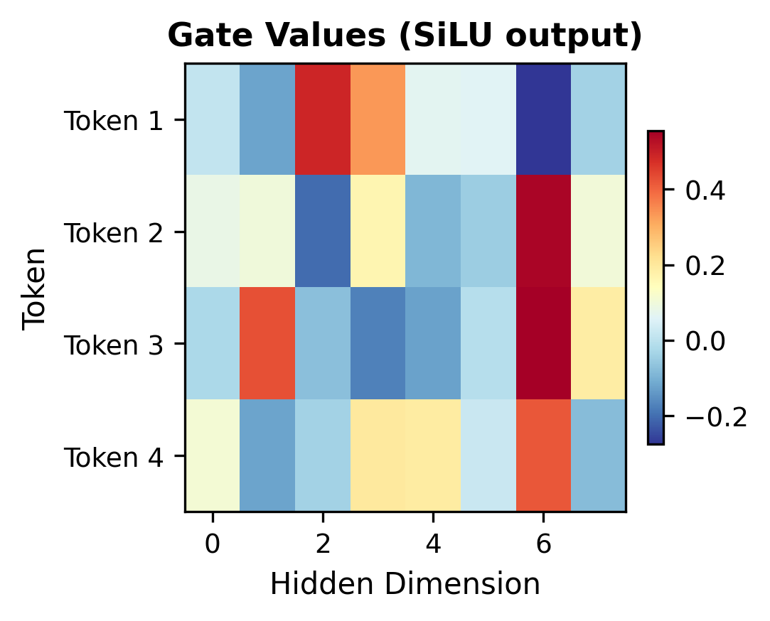
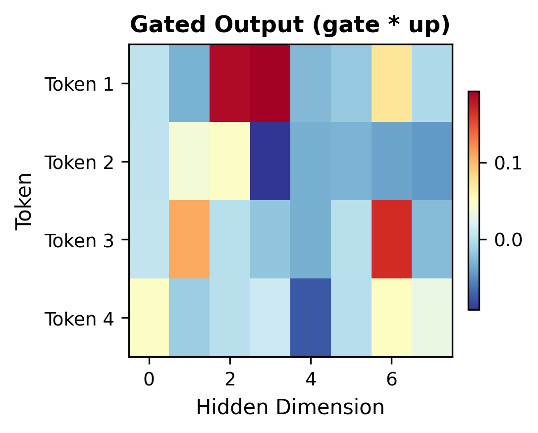
The heatmaps illustrate the gating mechanism's selective nature. Notice how dimensions with near-zero gate values (blue) suppress the corresponding up-projection values, while high gate values (red) allow information to pass through. This selective filtering gives SwiGLU its expressive advantage over simple activations.

Here's the implementation:

In[6]:

Code

class SwiGLUFFN:
    """
    Feed-forward network with SwiGLU activation.

    Uses gated linear units: output = (SiLU(x @ W_gate) * (x @ W_up)) @ W_down
    This is the standard FFN in LLaMA, Mistral, and similar models.
    """

    def __init__(self, d_model, d_ff):
        """
        Args:
            d_model: Model dimension
            d_ff: Hidden dimension of the FFN
        """
        self.d_model = d_model
        self.d_ff = d_ff

        # Initialize weights
        scale_up = np.sqrt(2.0 / (d_model + d_ff))
        scale_down = np.sqrt(2.0 / (d_ff + d_model))

        self.W_gate = np.random.randn(d_model, d_ff) * scale_up
        self.W_up = np.random.randn(d_model, d_ff) * scale_up
        self.W_down = np.random.randn(d_ff, d_model) * scale_down

    def __call__(self, x):
        """
        Apply SwiGLU feed-forward transformation.

        Args:
            x: Input tensor of shape (..., d_model)

        Returns:
            Output tensor of shape (..., d_model)
        """
        # Gate and up projections
        gate = silu(x @ self.W_gate)
        up = x @ self.W_up

        # Element-wise gating
        hidden = gate * up

        # Down projection
        output = hidden @ self.W_down

        return output

class SwiGLUFFN:
    """
    Feed-forward network with SwiGLU activation.

    Uses gated linear units: output = (SiLU(x @ W_gate) * (x @ W_up)) @ W_down
    This is the standard FFN in LLaMA, Mistral, and similar models.
    """

    def __init__(self, d_model, d_ff):
        """
        Args:
            d_model: Model dimension
            d_ff: Hidden dimension of the FFN
        """
        self.d_model = d_model
        self.d_ff = d_ff

        # Initialize weights
        scale_up = np.sqrt(2.0 / (d_model + d_ff))
        scale_down = np.sqrt(2.0 / (d_ff + d_model))

        self.W_gate = np.random.randn(d_model, d_ff) * scale_up
        self.W_up = np.random.randn(d_model, d_ff) * scale_up
        self.W_down = np.random.randn(d_ff, d_model) * scale_down

    def __call__(self, x):
        """
        Apply SwiGLU feed-forward transformation.

        Args:
            x: Input tensor of shape (..., d_model)

        Returns:
            Output tensor of shape (..., d_model)
        """
        # Gate and up projections
        gate = silu(x @ self.W_gate)
        up = x @ self.W_up

        # Element-wise gating
        hidden = gate * up

        # Down projection
        output = hidden @ self.W_down

        return output

We'll also implement a standard (non-gated) FFN for comparison. The standard FFN uses a simpler two-layer structure:

\text{FFN}(\mathbf{x}) = \text{activation}(\mathbf{x}\mathbf{W}_1)\mathbf{W}_2

where:

$\mathbf{W}_1 \in \mathbb{R}^{d \times d_{\text{ff}}}$ : projects from model dimension to hidden dimension
$\mathbf{W}_2 \in \mathbb{R}^{d_{\text{ff}} \times d}$ : projects back to model dimension
$\text{activation}$ : typically GELU in GPT-style models

In[7]:

Code

class StandardFFN:
    """
    Standard two-layer feed-forward network.

    Implements: FFN(x) = activation(x @ W1) @ W2
    """

    def __init__(self, d_model, d_ff, activation=gelu):
        """
        Args:
            d_model: Model dimension
            d_ff: Hidden dimension
            activation: Nonlinear activation function
        """
        self.d_model = d_model
        self.d_ff = d_ff
        self.activation = activation

        # Initialize weights
        scale1 = np.sqrt(2.0 / (d_model + d_ff))
        scale2 = np.sqrt(2.0 / (d_ff + d_model))

        self.W1 = np.random.randn(d_model, d_ff) * scale1
        self.W2 = np.random.randn(d_ff, d_model) * scale2

    def __call__(self, x):
        """Apply feed-forward transformation."""
        hidden = self.activation(x @ self.W1)
        output = hidden @ self.W2
        return output

class StandardFFN:
    """
    Standard two-layer feed-forward network.

    Implements: FFN(x) = activation(x @ W1) @ W2
    """

    def __init__(self, d_model, d_ff, activation=gelu):
        """
        Args:
            d_model: Model dimension
            d_ff: Hidden dimension
            activation: Nonlinear activation function
        """
        self.d_model = d_model
        self.d_ff = d_ff
        self.activation = activation

        # Initialize weights
        scale1 = np.sqrt(2.0 / (d_model + d_ff))
        scale2 = np.sqrt(2.0 / (d_ff + d_model))

        self.W1 = np.random.randn(d_model, d_ff) * scale1
        self.W2 = np.random.randn(d_ff, d_model) * scale2

    def __call__(self, x):
        """Apply feed-forward transformation."""
        hidden = self.activation(x @ self.W1)
        output = hidden @ self.W2
        return output

Assembling the Transformer BlockLink Copied

Now we combine these components into a complete transformer block. The key is getting the ordering right: normalize before each sublayer, apply the transformation, then add the residual.

In[8]:

Code

class TransformerBlock:
    """
    Complete transformer block with pre-normalization.

    Architecture:
        x -> RMSNorm -> Attention -> +x -> RMSNorm -> FFN -> +

    This is the standard block structure used in GPT-2/3, LLaMA, etc.
    """

    def __init__(self, d_model, n_heads, d_ff, use_swiglu=True):
        """
        Args:
            d_model: Model dimension
            n_heads: Number of attention heads
            d_ff: Feed-forward hidden dimension
            use_swiglu: Whether to use SwiGLU (True) or standard FFN (False)
        """
        self.d_model = d_model
        self.n_heads = n_heads
        self.d_ff = d_ff

        # Normalization layers (one before each sublayer)
        self.norm1 = RMSNorm(d_model)
        self.norm2 = RMSNorm(d_model)

        # Attention sublayer
        self.attention = MultiHeadSelfAttention(d_model, n_heads)

        # Feed-forward sublayer
        if use_swiglu:
            self.ffn = SwiGLUFFN(d_model, d_ff)
        else:
            self.ffn = StandardFFN(d_model, d_ff)

    def __call__(self, x, mask=None):
        """
        Process input through the transformer block.

        Args:
            x: Input tensor of shape (seq_len, d_model)
            mask: Optional causal mask for attention

        Returns:
            Output tensor of shape (seq_len, d_model)
        """
        # Attention sublayer with pre-norm and residual
        normed = self.norm1(x)
        attn_out = self.attention(normed, mask)
        h = x + attn_out  # Residual connection

        # FFN sublayer with pre-norm and residual
        normed = self.norm2(h)
        ffn_out = self.ffn(normed)
        y = h + ffn_out  # Residual connection

        return y

    def num_parameters(self):
        """Count total parameters in the block."""
        # Normalization: 2 * d_model (two RMSNorm layers)
        norm_params = 2 * self.d_model

        # Attention: 4 * d_model^2 (Q, K, V, O projections)
        attn_params = 4 * self.d_model * self.d_model

        # FFN: depends on variant
        if isinstance(self.ffn, SwiGLUFFN):
            # SwiGLU: 3 * d_model * d_ff (gate, up, down)
            ffn_params = 3 * self.d_model * self.d_ff
        else:
            # Standard: 2 * d_model * d_ff (W1, W2)
            ffn_params = 2 * self.d_model * self.d_ff

        return norm_params + attn_params + ffn_params

class TransformerBlock:
    """
    Complete transformer block with pre-normalization.

    Architecture:
        x -> RMSNorm -> Attention -> +x -> RMSNorm -> FFN -> +

    This is the standard block structure used in GPT-2/3, LLaMA, etc.
    """

    def __init__(self, d_model, n_heads, d_ff, use_swiglu=True):
        """
        Args:
            d_model: Model dimension
            n_heads: Number of attention heads
            d_ff: Feed-forward hidden dimension
            use_swiglu: Whether to use SwiGLU (True) or standard FFN (False)
        """
        self.d_model = d_model
        self.n_heads = n_heads
        self.d_ff = d_ff

        # Normalization layers (one before each sublayer)
        self.norm1 = RMSNorm(d_model)
        self.norm2 = RMSNorm(d_model)

        # Attention sublayer
        self.attention = MultiHeadSelfAttention(d_model, n_heads)

        # Feed-forward sublayer
        if use_swiglu:
            self.ffn = SwiGLUFFN(d_model, d_ff)
        else:
            self.ffn = StandardFFN(d_model, d_ff)

    def __call__(self, x, mask=None):
        """
        Process input through the transformer block.

        Args:
            x: Input tensor of shape (seq_len, d_model)
            mask: Optional causal mask for attention

        Returns:
            Output tensor of shape (seq_len, d_model)
        """
        # Attention sublayer with pre-norm and residual
        normed = self.norm1(x)
        attn_out = self.attention(normed, mask)
        h = x + attn_out  # Residual connection

        # FFN sublayer with pre-norm and residual
        normed = self.norm2(h)
        ffn_out = self.ffn(normed)
        y = h + ffn_out  # Residual connection

        return y

    def num_parameters(self):
        """Count total parameters in the block."""
        # Normalization: 2 * d_model (two RMSNorm layers)
        norm_params = 2 * self.d_model

        # Attention: 4 * d_model^2 (Q, K, V, O projections)
        attn_params = 4 * self.d_model * self.d_model

        # FFN: depends on variant
        if isinstance(self.ffn, SwiGLUFFN):
            # SwiGLU: 3 * d_model * d_ff (gate, up, down)
            ffn_params = 3 * self.d_model * self.d_ff
        else:
            # Standard: 2 * d_model * d_ff (W1, W2)
            ffn_params = 2 * self.d_model * self.d_ff

        return norm_params + attn_params + ffn_params

Let's test the block and examine its behavior:

In[9]:

Code

# Create a transformer block with typical hyperparameters
d_model = 512
n_heads = 8
d_ff = 1376  # ~2.7x for SwiGLU (equivalent capacity to 4x standard)

np.random.seed(42)
block = TransformerBlock(d_model, n_heads, d_ff, use_swiglu=True)

# Create sample input: 16 tokens with 512-dimensional representations
seq_len = 16
x = np.random.randn(seq_len, d_model) * 0.02  # Small init like embeddings

# Process through the block
y = block(x)

# Create a transformer block with typical hyperparameters
d_model = 512
n_heads = 8
d_ff = 1376  # ~2.7x for SwiGLU (equivalent capacity to 4x standard)

np.random.seed(42)
block = TransformerBlock(d_model, n_heads, d_ff, use_swiglu=True)

# Create sample input: 16 tokens with 512-dimensional representations
seq_len = 16
x = np.random.randn(seq_len, d_model) * 0.02  # Small init like embeddings

# Process through the block
y = block(x)

Out[10]:

Console

Transformer Block Test
==================================================

Configuration:
  d_model: 512
  n_heads: 8
  d_ff: 1376
  FFN type: SwiGLU
  Total parameters: 3,163,136

Input/Output:
  Input shape: (16, 512)
  Output shape: (16, 512)
  Input mean: 0.000532, std: 0.019921
  Output mean: -0.018330, std: 0.526414

The block preserves the shape of its input: 16 tokens with 512 dimensions go in, and 16 tokens with 512 dimensions come out. The output statistics differ from the input, reflecting the transformations applied by attention and the FFN.

To understand how the block transforms representations, let's compare the input and output for each token:

Out[11]:

Visualization

Histogram comparing input and output activation distributions. — Distribution of activation values across all tokens and dimensions.

Bar chart comparing input and output L2 norms per token. — Per-token representation magnitudes showing how the block reshapes each token's embedding.

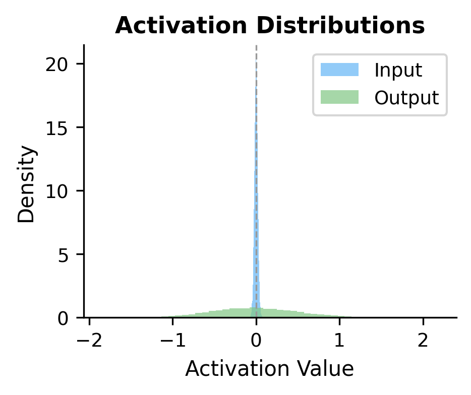
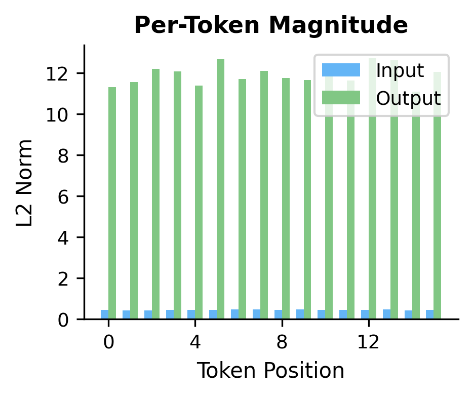
The histograms show that the block broadens the distribution of activation values, while the per-token norms reveal that different tokens are transformed by varying amounts. This position-dependent transformation is a signature of the attention mechanism, which allows tokens to selectively incorporate information from other positions.

Visualizing the Block StructureLink Copied

The component relationships become clearer with a visual diagram:

Out[12]:

Visualization

Block diagram showing transformer block with RMSNorm, attention, and FFN components connected by residual paths. — Complete transformer block structure with pre-normalization. The input flows through two sublayers (attention and FFN), each wrapped with normalization and a residual connection. The residual path (blue arrows) bypasses the sublayer, providing direct gradient flow.

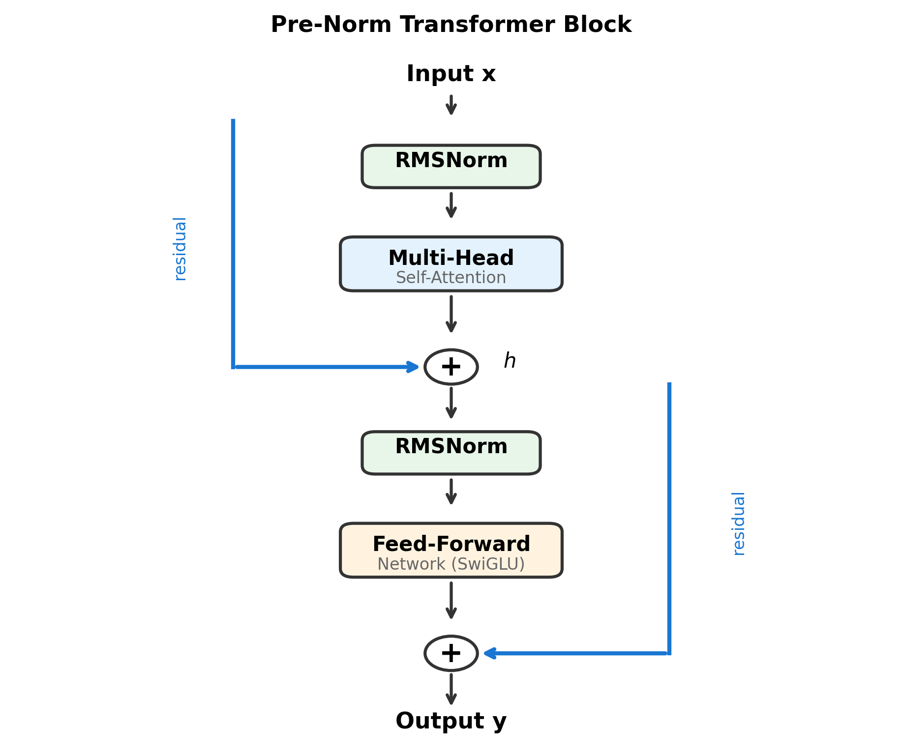
The diagram makes the pre-norm pattern explicit. At each sublayer, the input first passes through RMSNorm, then through the main transformation (attention or FFN), and finally the result is added back to the original input via the residual connection. The blue residual paths bypass the transformations entirely, ensuring gradients can flow directly from output to input.

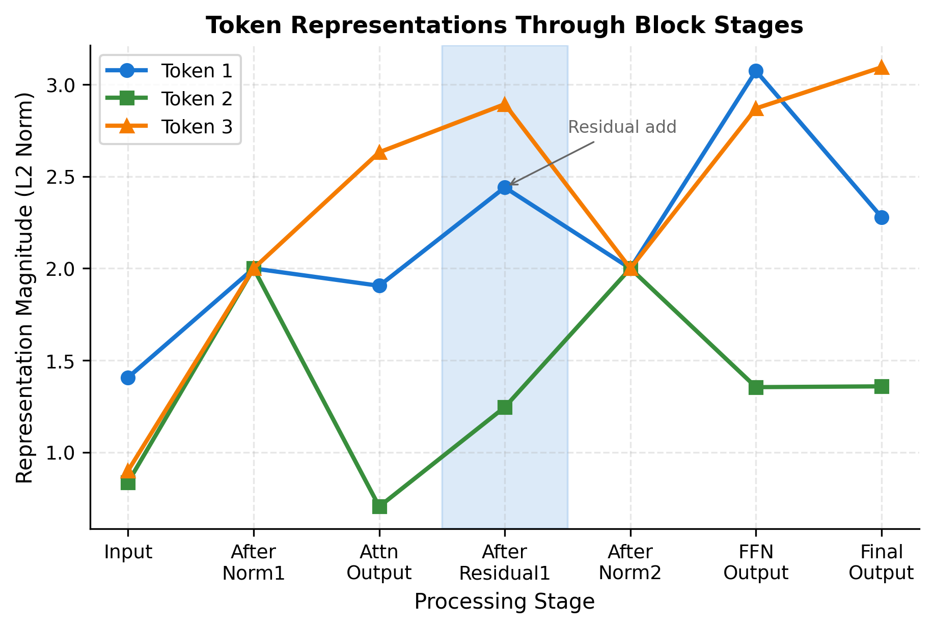
A Worked Example: Token by TokenLink Copied

To truly understand how data flows through a transformer block, let's trace a small concrete example with actual numbers. We'll use a tiny configuration so you can follow each computation:

$d_{\text{model}} = 4$ : each token is represented by just 4 numbers
$n_{\text{heads}} = 2$ : we split attention into 2 parallel heads
$d_{\text{ff}} = 8$ : the FFN's hidden layer has 8 dimensions
$n = 3$ : our sequence contains 3 tokens

In[13]:

Code

# Tiny configuration for hand-traceable computation
d_model_tiny = 4
n_heads_tiny = 2
d_ff_tiny = 8
seq_len_tiny = 3

np.random.seed(123)


# Create a tiny transformer block with standard FFN for simplicity
class TinyTransformerBlock:
    """Minimal transformer block for demonstration."""

    def __init__(self):
        self.d_model = d_model_tiny

        # RMSNorm weights (all ones for simplicity)
        self.norm1_weight = np.ones(d_model_tiny)
        self.norm2_weight = np.ones(d_model_tiny)

        # Attention weights (small random values)
        scale = 0.5
        self.W_q = np.random.randn(d_model_tiny, d_model_tiny) * scale
        self.W_k = np.random.randn(d_model_tiny, d_model_tiny) * scale
        self.W_v = np.random.randn(d_model_tiny, d_model_tiny) * scale
        self.W_o = np.random.randn(d_model_tiny, d_model_tiny) * scale

        # FFN weights
        self.W1 = np.random.randn(d_model_tiny, d_ff_tiny) * scale
        self.W2 = np.random.randn(d_ff_tiny, d_model_tiny) * scale

    def rmsnorm(self, x, weight):
        """Apply RMSNorm."""
        rms = np.sqrt(np.mean(x**2, axis=-1, keepdims=True) + 1e-6)
        return weight * (x / rms)

    def attention(self, x):
        """Simplified single-head attention for demonstration."""
        Q = x @ self.W_q
        K = x @ self.W_k
        V = x @ self.W_v

        # Attention scores
        scale = np.sqrt(self.d_model)
        scores = (Q @ K.T) / scale
        attn_weights = softmax(scores, axis=-1)

        # Apply attention
        context = attn_weights @ V
        output = context @ self.W_o

        return output, attn_weights

    def ffn(self, x):
        """Standard FFN with GELU."""
        hidden = gelu(x @ self.W1)
        output = hidden @ self.W2
        return output, hidden

    def forward_with_intermediates(self, x):
        """Forward pass returning all intermediate values."""
        intermediates = {"input": x.copy()}

        # First sublayer: attention
        x_norm1 = self.rmsnorm(x, self.norm1_weight)
        intermediates["after_norm1"] = x_norm1.copy()

        attn_out, attn_weights = self.attention(x_norm1)
        intermediates["attention_output"] = attn_out.copy()
        intermediates["attention_weights"] = attn_weights.copy()

        h = x + attn_out  # Residual
        intermediates["after_residual1"] = h.copy()

        # Second sublayer: FFN
        h_norm = self.rmsnorm(h, self.norm2_weight)
        intermediates["after_norm2"] = h_norm.copy()

        ffn_out, ffn_hidden = self.ffn(h_norm)
        intermediates["ffn_hidden"] = ffn_hidden.copy()
        intermediates["ffn_output"] = ffn_out.copy()

        y = h + ffn_out  # Residual
        intermediates["output"] = y.copy()

        return y, intermediates


# Create tiny block and sample input
tiny_block = TinyTransformerBlock()
x_tiny = np.array(
    [[1.0, 0.5, -0.3, 0.8], [-0.2, 0.7, 0.4, -0.1], [0.6, -0.4, 0.2, 0.5]]
)

# Forward pass with intermediates
output_tiny, intermediates = tiny_block.forward_with_intermediates(x_tiny)

# Tiny configuration for hand-traceable computation
d_model_tiny = 4
n_heads_tiny = 2
d_ff_tiny = 8
seq_len_tiny = 3

np.random.seed(123)


# Create a tiny transformer block with standard FFN for simplicity
class TinyTransformerBlock:
    """Minimal transformer block for demonstration."""

    def __init__(self):
        self.d_model = d_model_tiny

        # RMSNorm weights (all ones for simplicity)
        self.norm1_weight = np.ones(d_model_tiny)
        self.norm2_weight = np.ones(d_model_tiny)

        # Attention weights (small random values)
        scale = 0.5
        self.W_q = np.random.randn(d_model_tiny, d_model_tiny) * scale
        self.W_k = np.random.randn(d_model_tiny, d_model_tiny) * scale
        self.W_v = np.random.randn(d_model_tiny, d_model_tiny) * scale
        self.W_o = np.random.randn(d_model_tiny, d_model_tiny) * scale

        # FFN weights
        self.W1 = np.random.randn(d_model_tiny, d_ff_tiny) * scale
        self.W2 = np.random.randn(d_ff_tiny, d_model_tiny) * scale

    def rmsnorm(self, x, weight):
        """Apply RMSNorm."""
        rms = np.sqrt(np.mean(x**2, axis=-1, keepdims=True) + 1e-6)
        return weight * (x / rms)

    def attention(self, x):
        """Simplified single-head attention for demonstration."""
        Q = x @ self.W_q
        K = x @ self.W_k
        V = x @ self.W_v

        # Attention scores
        scale = np.sqrt(self.d_model)
        scores = (Q @ K.T) / scale
        attn_weights = softmax(scores, axis=-1)

        # Apply attention
        context = attn_weights @ V
        output = context @ self.W_o

        return output, attn_weights

    def ffn(self, x):
        """Standard FFN with GELU."""
        hidden = gelu(x @ self.W1)
        output = hidden @ self.W2
        return output, hidden

    def forward_with_intermediates(self, x):
        """Forward pass returning all intermediate values."""
        intermediates = {"input": x.copy()}

        # First sublayer: attention
        x_norm1 = self.rmsnorm(x, self.norm1_weight)
        intermediates["after_norm1"] = x_norm1.copy()

        attn_out, attn_weights = self.attention(x_norm1)
        intermediates["attention_output"] = attn_out.copy()
        intermediates["attention_weights"] = attn_weights.copy()

        h = x + attn_out  # Residual
        intermediates["after_residual1"] = h.copy()

        # Second sublayer: FFN
        h_norm = self.rmsnorm(h, self.norm2_weight)
        intermediates["after_norm2"] = h_norm.copy()

        ffn_out, ffn_hidden = self.ffn(h_norm)
        intermediates["ffn_hidden"] = ffn_hidden.copy()
        intermediates["ffn_output"] = ffn_out.copy()

        y = h + ffn_out  # Residual
        intermediates["output"] = y.copy()

        return y, intermediates


# Create tiny block and sample input
tiny_block = TinyTransformerBlock()
x_tiny = np.array(
    [[1.0, 0.5, -0.3, 0.8], [-0.2, 0.7, 0.4, -0.1], [0.6, -0.4, 0.2, 0.5]]
)

# Forward pass with intermediates
output_tiny, intermediates = tiny_block.forward_with_intermediates(x_tiny)

Out[14]:

Console

Transformer Block Walkthrough
============================================================

Input (3 tokens, 4 dimensions):
[[ 1.   0.5 -0.3  0.8]
 [-0.2  0.7  0.4 -0.1]
 [ 0.6 -0.4  0.2  0.5]]

--- ATTENTION SUBLAYER ---

After RMSNorm (normalized input):
[[ 1.421  0.711 -0.426  1.137]
 [-0.478  1.673  0.956 -0.239]
 [ 1.333 -0.889  0.444  1.111]]

Attention weights (which tokens attend to which):
[[0.394 0.183 0.423]
 [0.475 0.464 0.06 ]
 [0.189 0.051 0.76 ]]

Attention output:
[[-0.266  0.531  1.614  0.822]
 [-0.257 -0.136  0.606  0.212]
 [-0.446  0.945  2.172  1.057]]

After residual connection (input + attention output):
[[ 0.734  1.031  1.314  1.622]
 [-0.457  0.564  1.006  0.112]
 [ 0.154  0.545  2.372  1.557]]

--- FFN SUBLAYER ---

After RMSNorm:
[[ 0.601  0.845  1.076  1.329]
 [-0.735  0.905  1.615  0.18 ]
 [ 0.107  0.377  1.639  1.076]]

FFN hidden activations (8 dimensions, showing first 4):
[[ 2.976 -0.152  0.605 -0.019]
 [ 1.069 -0.122  0.317  0.944]
 [ 2.43  -0.167  1.493  0.092]]

FFN output:
[[-1.806 -1.845  0.525 -1.585]
 [-0.393 -1.275 -0.231  0.016]
 [-1.369 -1.482  0.275 -2.023]]

--- FINAL OUTPUT ---

Block output (intermediate + FFN output):
[[-1.072 -0.814  1.839  0.037]
 [-0.85  -0.711  0.775  0.128]
 [-1.215 -0.937  2.647 -0.466]]

Let's visualize how each token's representation evolves through the block stages:

Out[15]:

Visualization

Line plot showing 3 tokens' L2 norms changing through 6 processing stages of the transformer block. — Evolution of token representations through the transformer block. Each line traces one token's representation magnitude as it passes through normalization, attention, residual addition, and FFN stages. The residual connections visibly preserve and augment the representations.

Understanding the Attention WeightsLink Copied

The attention weights matrix shows how each token attends to others in the sequence. Let's visualize this pattern:

Out[16]:

Visualization

Heatmap showing 3x3 attention weight matrix with varying attention patterns per token. — Attention pattern from our worked example. Each row shows how one token distributes its attention across all tokens. Token 1 attends broadly, while Tokens 2 and 3 focus more on specific positions.

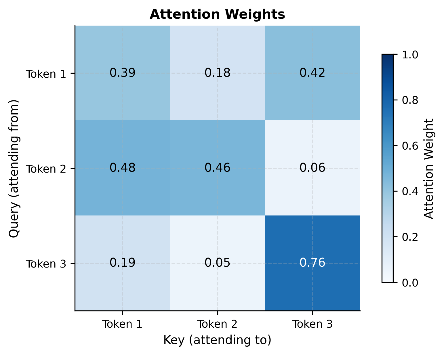
Each row in the attention matrix sums to 1.0 (due to softmax normalization). If we denote the attention weight from token $i$ to token $j$ as $\alpha_{ij}$ , then:

\sum_{j=1}^{n} \alpha_{ij} = 1 \quad \text{for all } i

where $n$ is the sequence length. This constraint ensures that each token's output is a valid weighted average of the value vectors from all positions. No attention weight can be negative, and the weights form a probability distribution over the sequence.

Tracing the Residual ContributionLink Copied

One key insight from residual connections is that the output preserves information from the input. Let's quantify this:

In[17]:

Code

# Decompose the output into residual and sublayer contributions
input_contribution = x_tiny  # Original input (passes through both residuals)
attn_contribution = intermediates["attention_output"]
ffn_contribution = intermediates["ffn_output"]

# The output is: input + attention_output + ffn_output
reconstructed = input_contribution + attn_contribution + ffn_contribution

# Decompose the output into residual and sublayer contributions
input_contribution = x_tiny  # Original input (passes through both residuals)
attn_contribution = intermediates["attention_output"]
ffn_contribution = intermediates["ffn_output"]

# The output is: input + attention_output + ffn_output
reconstructed = input_contribution + attn_contribution + ffn_contribution

Out[18]:

Console

Output Decomposition
==================================================

Original input contribution:
  Magnitude: 1.8682

Attention sublayer contribution:
  Magnitude: 3.3251

FFN sublayer contribution:
  Magnitude: 4.4187

Reconstruction check (should match output):
  Match: True

Relative contributions:
  Input: 19.4%
  Attention: 34.6%
  FFN: 46.0%

Out[19]:

Visualization

Horizontal stacked bar chart showing input, attention, and FFN contributions for 3 tokens. — Decomposition of transformer block output into its component contributions. The stacked bar chart shows how the final representation for each token combines the original input with additive contributions from attention and FFN sublayers.

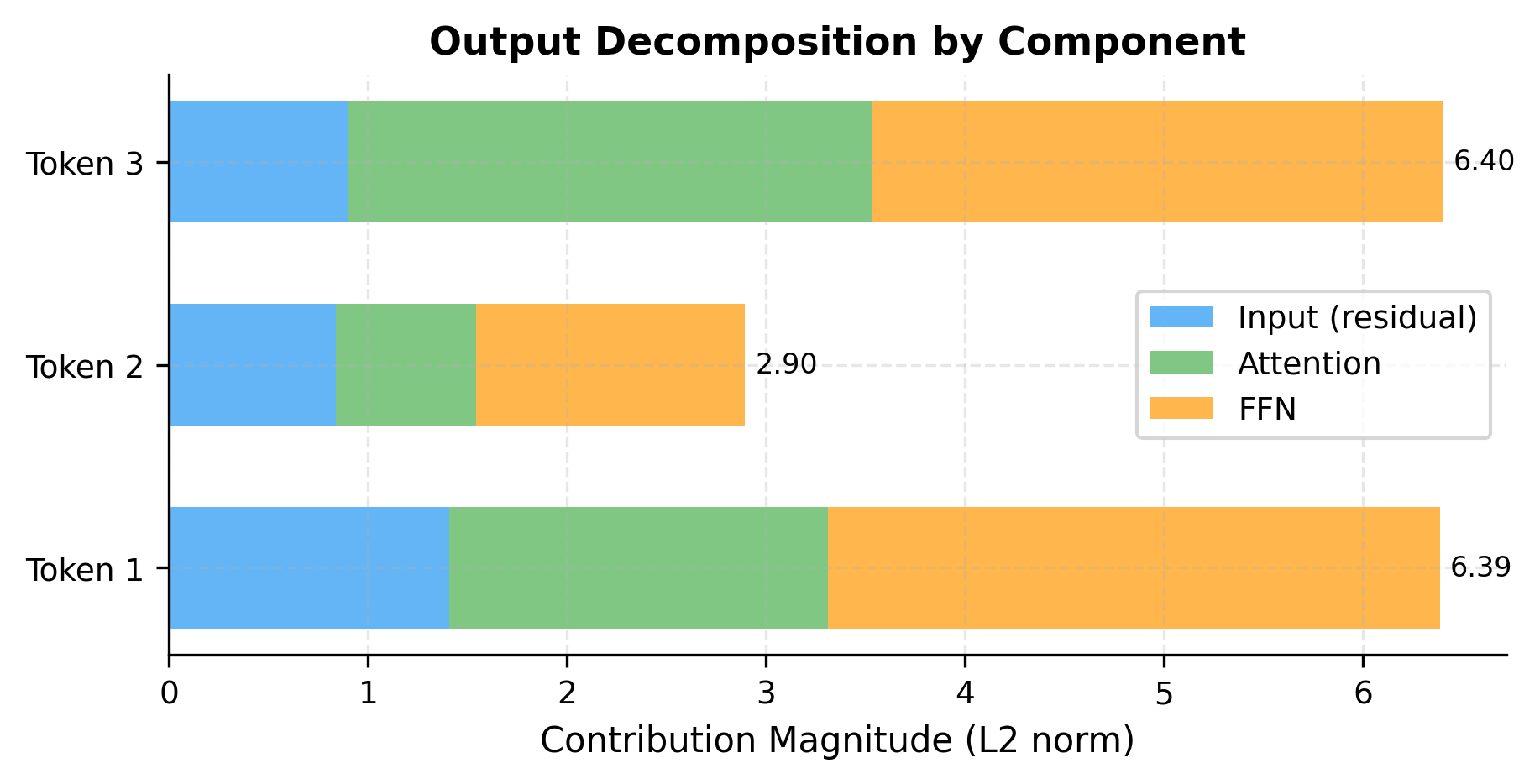
The decomposition reveals how each component contributes to the final representation. Mathematically, the output $\mathbf{y}$ can be written as:

\mathbf{y} = \mathbf{x} + \Delta_{\text{attn}} + \Delta_{\text{ffn}}

where:

$\mathbf{x}$ : the original input, which passes through both residual connections unchanged
$\Delta_{\text{attn}} = \text{Attention}(\text{Norm}(\mathbf{x}))$ : the attention sublayer's contribution
$\Delta_{\text{ffn}} = \text{FFN}(\text{Norm}(\mathbf{h}))$ : the FFN sublayer's contribution

The original input remains a substantial part of the output, demonstrating how residual connections preserve information while allowing sublayers to add refinements. This additive structure also explains why gradients flow easily backward through transformer blocks: they can bypass the nonlinear sublayers entirely via the residual paths.

Causal Masking for Decoder BlocksLink Copied

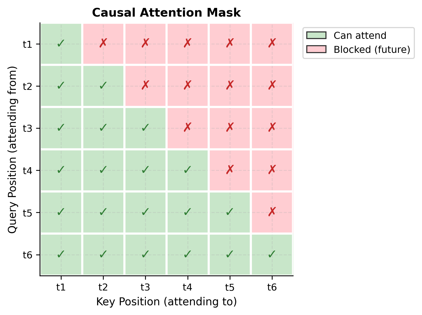
Language models like GPT are autoregressive: they generate tokens one at a time, with each token depending only on previous tokens. This requires causal masking in attention, preventing tokens from attending to future positions.

The causal mask modifies the attention score computation. Recall that attention scores between queries and keys are computed as:

\text{score}_{ij} = \frac{\mathbf{q}_i \cdot \mathbf{k}_j}{\sqrt{d_k}}

where:

$\mathbf{q}_i$ : the query vector for token at position $i$
$\mathbf{k}_j$ : the key vector for token at position $j$
$d_k$ : the dimension of the key vectors (used for scaling)

To prevent token $i$ from attending to any future token $j > i$ , we add a mask $M$ to the scores before applying softmax:

\text{masked\_score}_{ij} = \text{score}_{ij} + M_{ij}

where:

$M_{ij} = 0$ if $j \leq i$ (past or current positions, allowed)
$M_{ij} = -\infty$ if $j > i$ (future positions, blocked)

After softmax, positions with $-\infty$ scores become exactly zero, effectively removing them from the weighted average. The result is a triangular attention pattern where each token can only "see" itself and previous tokens:

In[20]:

Code

def create_causal_mask(seq_len):
    """
    Create causal attention mask.

    Returns a matrix where position (i, j) is -inf if j > i (future position),
    and 0 otherwise. Adding this to attention scores before softmax
    ensures tokens cannot attend to future positions.
    """
    mask = np.triu(np.ones((seq_len, seq_len)) * float("-inf"), k=1)
    return mask


# Example mask for 4 tokens
mask_example = create_causal_mask(4)

def create_causal_mask(seq_len):
    """
    Create causal attention mask.

    Returns a matrix where position (i, j) is -inf if j > i (future position),
    and 0 otherwise. Adding this to attention scores before softmax
    ensures tokens cannot attend to future positions.
    """
    mask = np.triu(np.ones((seq_len, seq_len)) * float("-inf"), k=1)
    return mask


# Example mask for 4 tokens
mask_example = create_causal_mask(4)

Out[21]:

Console

Causal Mask (4 tokens):
(0 = can attend, -inf = cannot attend)

  0  -∞  -∞  -∞
  0  0  -∞  -∞
  0  0  0  -∞
  0  0  0  0

Out[22]:

Visualization

Triangular heatmap showing causal mask pattern with lower triangle green (allowed) and upper triangle red (blocked). — Causal attention mask for a 6-token sequence. Green cells indicate allowed attention (token can see that position), red cells indicate blocked attention (future positions). Each token can only attend to itself and previous tokens.

Decoder Block ImplementationLink Copied

A decoder block is identical to the standard block, but with causal masking applied during attention:

In[23]:

Code

class DecoderBlock(TransformerBlock):
    """
    Transformer decoder block with causal masking.

    Identical to TransformerBlock but automatically applies
    causal masking to prevent attending to future positions.
    """

    def __call__(self, x):
        """
        Process input through decoder block.

        Args:
            x: Input tensor of shape (seq_len, d_model)

        Returns:
            Output tensor of shape (seq_len, d_model)
        """
        seq_len = x.shape[0]

        # Create causal mask
        mask = create_causal_mask(seq_len)

        # Use parent class forward with mask
        return super().__call__(x, mask=mask)


# Test decoder block
np.random.seed(42)
decoder_block = DecoderBlock(d_model=256, n_heads=4, d_ff=688, use_swiglu=True)

x_test = np.random.randn(8, 256) * 0.02
y_test = decoder_block(x_test)

class DecoderBlock(TransformerBlock):
    """
    Transformer decoder block with causal masking.

    Identical to TransformerBlock but automatically applies
    causal masking to prevent attending to future positions.
    """

    def __call__(self, x):
        """
        Process input through decoder block.

        Args:
            x: Input tensor of shape (seq_len, d_model)

        Returns:
            Output tensor of shape (seq_len, d_model)
        """
        seq_len = x.shape[0]

        # Create causal mask
        mask = create_causal_mask(seq_len)

        # Use parent class forward with mask
        return super().__call__(x, mask=mask)


# Test decoder block
np.random.seed(42)
decoder_block = DecoderBlock(d_model=256, n_heads=4, d_ff=688, use_swiglu=True)

x_test = np.random.randn(8, 256) * 0.02
y_test = decoder_block(x_test)

Out[24]:

Console

Decoder Block Test
========================================
Input shape: (8, 256)
Output shape: (8, 256)
Causal masking: enabled
Parameters: 791,040

Stacking Blocks: Building a Complete ModelLink Copied

A transformer model stacks multiple blocks in sequence. The output of one block becomes the input to the next, with each block refining the representations:

In[25]:

Code

class TransformerStack:
    """
    Stack of transformer blocks forming a complete encoder or decoder.
    """

    def __init__(
        self,
        n_layers,
        d_model,
        n_heads,
        d_ff,
        use_swiglu=True,
        is_decoder=False,
    ):
        """
        Args:
            n_layers: Number of transformer blocks
            d_model: Model dimension
            n_heads: Number of attention heads
            d_ff: Feed-forward hidden dimension
            use_swiglu: Whether to use SwiGLU FFN
            is_decoder: Whether to apply causal masking
        """
        self.n_layers = n_layers
        self.is_decoder = is_decoder

        # Create blocks
        if is_decoder:
            self.blocks = [
                DecoderBlock(d_model, n_heads, d_ff, use_swiglu)
                for _ in range(n_layers)
            ]
        else:
            self.blocks = [
                TransformerBlock(d_model, n_heads, d_ff, use_swiglu)
                for _ in range(n_layers)
            ]

        # Final normalization (after all blocks)
        self.final_norm = RMSNorm(d_model)

    def __call__(self, x):
        """
        Process input through all transformer blocks.

        Args:
            x: Input tensor of shape (seq_len, d_model)

        Returns:
            Output tensor of shape (seq_len, d_model)
        """
        # Pass through each block sequentially
        for block in self.blocks:
            x = block(x)

        # Final normalization
        x = self.final_norm(x)

        return x

    def num_parameters(self):
        """Total parameters in the stack."""
        block_params = sum(block.num_parameters() for block in self.blocks)
        # Final norm adds d_model parameters
        return block_params + self.blocks[0].d_model


# Create a small transformer stack
np.random.seed(42)
transformer = TransformerStack(
    n_layers=6,
    d_model=256,
    n_heads=4,
    d_ff=688,
    use_swiglu=True,
    is_decoder=True,
)

class TransformerStack:
    """
    Stack of transformer blocks forming a complete encoder or decoder.
    """

    def __init__(
        self,
        n_layers,
        d_model,
        n_heads,
        d_ff,
        use_swiglu=True,
        is_decoder=False,
    ):
        """
        Args:
            n_layers: Number of transformer blocks
            d_model: Model dimension
            n_heads: Number of attention heads
            d_ff: Feed-forward hidden dimension
            use_swiglu: Whether to use SwiGLU FFN
            is_decoder: Whether to apply causal masking
        """
        self.n_layers = n_layers
        self.is_decoder = is_decoder

        # Create blocks
        if is_decoder:
            self.blocks = [
                DecoderBlock(d_model, n_heads, d_ff, use_swiglu)
                for _ in range(n_layers)
            ]
        else:
            self.blocks = [
                TransformerBlock(d_model, n_heads, d_ff, use_swiglu)
                for _ in range(n_layers)
            ]

        # Final normalization (after all blocks)
        self.final_norm = RMSNorm(d_model)

    def __call__(self, x):
        """
        Process input through all transformer blocks.

        Args:
            x: Input tensor of shape (seq_len, d_model)

        Returns:
            Output tensor of shape (seq_len, d_model)
        """
        # Pass through each block sequentially
        for block in self.blocks:
            x = block(x)

        # Final normalization
        x = self.final_norm(x)

        return x

    def num_parameters(self):
        """Total parameters in the stack."""
        block_params = sum(block.num_parameters() for block in self.blocks)
        # Final norm adds d_model parameters
        return block_params + self.blocks[0].d_model


# Create a small transformer stack
np.random.seed(42)
transformer = TransformerStack(
    n_layers=6,
    d_model=256,
    n_heads=4,
    d_ff=688,
    use_swiglu=True,
    is_decoder=True,
)

Out[26]:

Console

Transformer Stack Configuration
==================================================
  Layers: 6
  d_model: 256
  n_heads: 4
  d_ff: 688
  FFN type: SwiGLU
  Type: Decoder (causal)
  Total parameters: 4,746,496

Let's trace how representations evolve through the stack:

In[27]:

Code

# Track representations through layers
def trace_through_stack(stack, x):
    """Collect representations after each layer."""
    representations = [x.copy()]

    current = x
    for block in stack.blocks:
        current = block(current)
        representations.append(current.copy())

    # After final norm
    final = stack.final_norm(current)
    representations.append(final.copy())

    return representations


# Trace through the stack
x_trace = np.random.randn(8, 256) * 0.02
layer_outputs = trace_through_stack(transformer, x_trace)

# Track representations through layers
def trace_through_stack(stack, x):
    """Collect representations after each layer."""
    representations = [x.copy()]

    current = x
    for block in stack.blocks:
        current = block(current)
        representations.append(current.copy())

    # After final norm
    final = stack.final_norm(current)
    representations.append(final.copy())

    return representations


# Trace through the stack
x_trace = np.random.randn(8, 256) * 0.02
layer_outputs = trace_through_stack(transformer, x_trace)

Out[28]:

Visualization

Line plot showing representation magnitude increasing slightly through 6 transformer layers plus final norm. — How representations evolve through a 6-layer transformer stack. The plot shows the mean L2 norm of token representations after each layer. The gradual increase reflects the accumulation of information via residual connections.

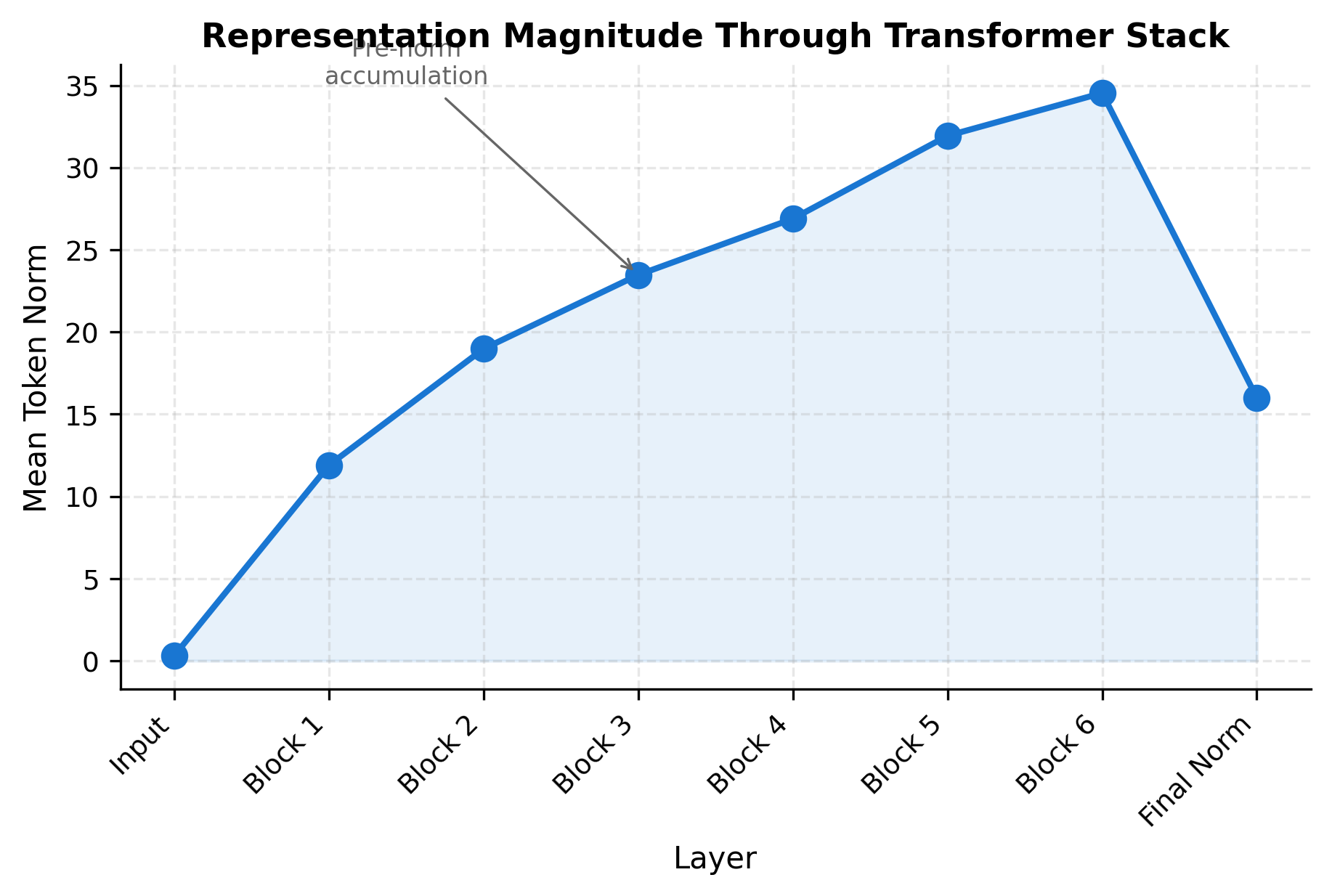
The visualization shows how pre-norm architectures allow representation magnitude to grow through the network. Each residual connection adds to the running sum. The final normalization (RMSNorm after all blocks) brings the representations back to a controlled scale before the output layer.

Parameter Breakdown by ComponentLink Copied

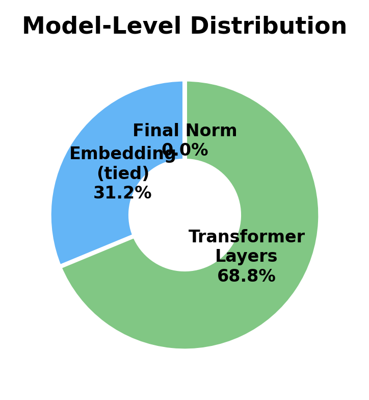
Understanding where parameters live helps with model analysis and optimization. Let's break down a complete model:

In[29]:

Code

def analyze_model_parameters(n_layers, d_model, n_heads, d_ff, vocab_size):
    """
    Analyze parameter distribution in a transformer language model.

    Returns dict with parameter counts for each component.
    """
    analysis = {}

    # Embedding (input and output tied)
    analysis["embedding"] = vocab_size * d_model

    # Per-layer components
    per_layer = {}

    # RMSNorm: 2 per layer (attention + FFN) with d_model params each
    per_layer["norm"] = 2 * d_model

    # Attention: Q, K, V, O projections
    per_layer["attention"] = 4 * d_model * d_model

    # SwiGLU FFN: gate, up, down projections
    per_layer["ffn"] = 3 * d_model * d_ff

    per_layer["total"] = sum(per_layer.values())

    # Total for all layers
    analysis["per_layer"] = per_layer
    analysis["all_layers"] = n_layers * per_layer["total"]

    # Final norm
    analysis["final_norm"] = d_model

    # LM head (often tied with embedding)
    analysis["lm_head"] = 0  # Tied with embedding

    # Total
    analysis["total"] = (
        analysis["embedding"] + analysis["all_layers"] + analysis["final_norm"]
    )

    return analysis


# Analyze a GPT-2 Small-like configuration
analysis = analyze_model_parameters(
    n_layers=12,
    d_model=768,
    n_heads=12,
    d_ff=2048,  # ~2.7x with SwiGLU
    vocab_size=50257,
)

def analyze_model_parameters(n_layers, d_model, n_heads, d_ff, vocab_size):
    """
    Analyze parameter distribution in a transformer language model.

    Returns dict with parameter counts for each component.
    """
    analysis = {}

    # Embedding (input and output tied)
    analysis["embedding"] = vocab_size * d_model

    # Per-layer components
    per_layer = {}

    # RMSNorm: 2 per layer (attention + FFN) with d_model params each
    per_layer["norm"] = 2 * d_model

    # Attention: Q, K, V, O projections
    per_layer["attention"] = 4 * d_model * d_model

    # SwiGLU FFN: gate, up, down projections
    per_layer["ffn"] = 3 * d_model * d_ff

    per_layer["total"] = sum(per_layer.values())

    # Total for all layers
    analysis["per_layer"] = per_layer
    analysis["all_layers"] = n_layers * per_layer["total"]

    # Final norm
    analysis["final_norm"] = d_model

    # LM head (often tied with embedding)
    analysis["lm_head"] = 0  # Tied with embedding

    # Total
    analysis["total"] = (
        analysis["embedding"] + analysis["all_layers"] + analysis["final_norm"]
    )

    return analysis


# Analyze a GPT-2 Small-like configuration
analysis = analyze_model_parameters(
    n_layers=12,
    d_model=768,
    n_heads=12,
    d_ff=2048,  # ~2.7x with SwiGLU
    vocab_size=50257,
)

Out[30]:

Console

Parameter Analysis (GPT-2 Small-like configuration)
=======================================================

Configuration:
  Layers: 12, d_model: 768, n_heads: 12, d_ff: 2048
  Vocabulary: 50,257 tokens

Per-layer breakdown:
  Norm        :        1,536 (  0.0%)
  Attention   :    2,359,296 ( 33.3%)
  Ffn         :    4,718,592 ( 66.7%)
  ──────────────────────────────
  Total       :    7,079,424

Model totals:
  Embedding:      38,597,376
  All layers:     84,953,088
  Final norm:            768
  ──────────────────────────────
  Total:         123,551,232

  (~124M parameters)

Out[31]:

Visualization

Donut chart showing embedding, transformer layers, and final norm as fractions of total parameters. — Model-level parameter distribution showing embedding and transformer layers.

Donut chart showing norm, attention, and FFN as fractions of per-layer parameters. — Per-layer parameter distribution showing FFN dominance over attention and normalization.

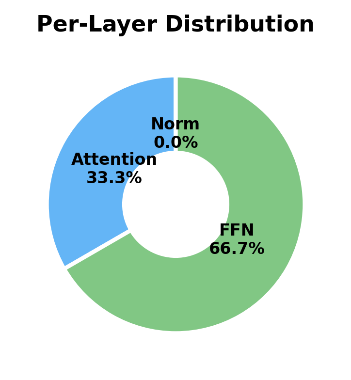
The analysis reveals that FFN parameters dominate within each transformer block. Let's quantify this for SwiGLU:

Attention parameters: $4 \times d_{\text{model}}^2$ (for Q, K, V, and O projections)
SwiGLU FFN parameters: $3 \times d_{\text{model}} \times d_{\text{ff}}$ (for gate, up, and down projections)

With typical SwiGLU expansion ( $d_{\text{ff}} \approx 2.7 \times d_{\text{model}}$ ), the FFN has about $8.1 \times d_{\text{model}}^2$ parameters versus attention's $4 \times d_{\text{model}}^2$ . This is roughly a 2:1 ratio, meaning FFN accounts for about 67% of each block's parameters. At the model level, the embedding layer is also significant: with vocabulary size $V$ , the embedding matrix has $V \times d_{\text{model}}$ parameters, which can exceed a single layer's parameters for large vocabularies.

Comparing Block ArchitecturesLink Copied

Different models use slightly different block configurations. Let's compare the major variants:

In[32]:

Code

# Define configurations for major architectures
architectures = {
    "GPT-2": {
        "norm_type": "LayerNorm",
        "norm_placement": "Pre-norm",
        "ffn_type": "Standard (GELU)",
        "ffn_expansion": 4.0,
        "attention_type": "Dense",
    },
    "LLaMA": {
        "norm_type": "RMSNorm",
        "norm_placement": "Pre-norm",
        "ffn_type": "SwiGLU",
        "ffn_expansion": 2.7,  # ~8/3 with gating
        "attention_type": "Dense + RoPE",
    },
    "Mistral": {
        "norm_type": "RMSNorm",
        "norm_placement": "Pre-norm",
        "ffn_type": "SwiGLU",
        "ffn_expansion": 2.7,
        "attention_type": "Sliding Window + GQA",
    },
    "BERT": {
        "norm_type": "LayerNorm",
        "norm_placement": "Post-norm",
        "ffn_type": "Standard (GELU)",
        "ffn_expansion": 4.0,
        "attention_type": "Dense (bidirectional)",
    },
}

# Define configurations for major architectures
architectures = {
    "GPT-2": {
        "norm_type": "LayerNorm",
        "norm_placement": "Pre-norm",
        "ffn_type": "Standard (GELU)",
        "ffn_expansion": 4.0,
        "attention_type": "Dense",
    },
    "LLaMA": {
        "norm_type": "RMSNorm",
        "norm_placement": "Pre-norm",
        "ffn_type": "SwiGLU",
        "ffn_expansion": 2.7,  # ~8/3 with gating
        "attention_type": "Dense + RoPE",
    },
    "Mistral": {
        "norm_type": "RMSNorm",
        "norm_placement": "Pre-norm",
        "ffn_type": "SwiGLU",
        "ffn_expansion": 2.7,
        "attention_type": "Sliding Window + GQA",
    },
    "BERT": {
        "norm_type": "LayerNorm",
        "norm_placement": "Post-norm",
        "ffn_type": "Standard (GELU)",
        "ffn_expansion": 4.0,
        "attention_type": "Dense (bidirectional)",
    },
}

Out[33]:

Console

Transformer Block Architecture Comparison
======================================================================

Component           GPT-2       LLaMA       Mistral     BERT        
----------------------------------------------------------------------
Norm Type           LayerNorm   RMSNorm     RMSNorm     LayerNorm   
Norm Placement      Pre-norm    Pre-norm    Pre-norm    Post-norm   
Ffn Type            Standard (GELU)SwiGLU      SwiGLU      Standard (GELU)
Ffn Expansion       4.0         x2.7         x2.7         x4.0         x
Attention Type      Dense       Dense + RoPESliding Window + GQADense (bidirectional)

The table highlights key design decisions that distinguish architectures:

Modern models (LLaMA, Mistral) use RMSNorm for efficiency and SwiGLU for improved FFN expressiveness
BERT is a notable exception, using post-norm placement (it predates the pre-norm stability insights)
FFN expansion is smaller with gated variants because gating effectively doubles the hidden dimension

To visualize how these architectural choices affect parameter allocation, let's compare parameter counts across different model scales:

Out[34]:

Visualization

Stacked area chart showing parameter counts for embedding, attention, and FFN components across different d_model values. — How transformer parameters scale with model size. As d_model increases, attention (which scales as d_model squared) and FFN (which scales as d_model times d_ff) grow at different rates. The embedding layer's relative contribution decreases for larger models with fixed vocabulary size.

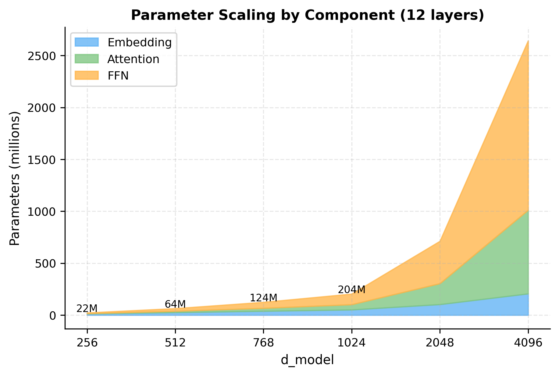
The scaling chart reveals an important insight: as models grow larger, the FFN becomes increasingly dominant. At $d_{\text{model}} = 4096$ , the FFN accounts for over 80% of transformer layer parameters. This explains why efficiency innovations (like Mixture of Experts) primarily target the FFN component.

Implementation: Production-Ready BlockLink Copied

Let's create a complete, configurable transformer block that supports all the variants we've discussed:

In[35]:

Code

class ConfigurableTransformerBlock:
    """
    Production-style transformer block with configurable components.

    Supports:
        - RMSNorm or LayerNorm
        - Pre-norm or post-norm placement
        - Standard or SwiGLU FFN
        - Optional causal masking
    """

    def __init__(self, config):
        """
        Args:
            config: dict with keys:
                - d_model: int, model dimension
                - n_heads: int, number of attention heads
                - d_ff: int, FFN hidden dimension
                - norm_type: 'rmsnorm' or 'layernorm'
                - norm_placement: 'pre' or 'post'
                - ffn_type: 'standard' or 'swiglu'
                - causal: bool, whether to apply causal masking
                - eps: float, norm epsilon (default 1e-6)
        """
        self.config = config
        self.d_model = config["d_model"]
        self.causal = config.get("causal", False)

        # Initialize normalization layers
        if config["norm_type"] == "rmsnorm":
            self.norm1 = RMSNorm(config["d_model"], config.get("eps", 1e-6))
            self.norm2 = RMSNorm(config["d_model"], config.get("eps", 1e-6))
        else:
            # Simplified LayerNorm for demo
            self.norm1 = self._create_layernorm(config["d_model"])
            self.norm2 = self._create_layernorm(config["d_model"])

        # Attention
        self.attention = MultiHeadSelfAttention(
            config["d_model"], config["n_heads"]
        )

        # FFN
        if config["ffn_type"] == "swiglu":
            self.ffn = SwiGLUFFN(config["d_model"], config["d_ff"])
        else:
            self.ffn = StandardFFN(config["d_model"], config["d_ff"])

        self.norm_placement = config["norm_placement"]

    def _create_layernorm(self, dim):
        """Create a simple LayerNorm."""

        class LayerNorm:
            def __init__(self, dim, eps=1e-6):
                self.weight = np.ones(dim)
                self.bias = np.zeros(dim)
                self.eps = eps

            def __call__(self, x):
                mean = x.mean(axis=-1, keepdims=True)
                var = x.var(axis=-1, keepdims=True)
                return (
                    self.weight * (x - mean) / np.sqrt(var + self.eps)
                    + self.bias
                )

        return LayerNorm(dim)

    def __call__(self, x):
        """Forward pass through the block."""
        seq_len = x.shape[0]
        mask = create_causal_mask(seq_len) if self.causal else None

        if self.norm_placement == "pre":
            # Pre-norm: Norm -> Sublayer -> Residual
            h = x + self.attention(self.norm1(x), mask)
            y = h + self.ffn(self.norm2(h))
        else:
            # Post-norm: Sublayer -> Residual -> Norm
            h = self.norm1(x + self.attention(x, mask))
            y = self.norm2(h + self.ffn(h))

        return y


# Create LLaMA-style block
llama_config = {
    "d_model": 256,
    "n_heads": 4,
    "d_ff": 688,
    "norm_type": "rmsnorm",
    "norm_placement": "pre",
    "ffn_type": "swiglu",
    "causal": True,
}

np.random.seed(42)
llama_block = ConfigurableTransformerBlock(llama_config)

# Test
x_config_test = np.random.randn(8, 256) * 0.02
y_config_test = llama_block(x_config_test)

class ConfigurableTransformerBlock:
    """
    Production-style transformer block with configurable components.

    Supports:
        - RMSNorm or LayerNorm
        - Pre-norm or post-norm placement
        - Standard or SwiGLU FFN
        - Optional causal masking
    """

    def __init__(self, config):
        """
        Args:
            config: dict with keys:
                - d_model: int, model dimension
                - n_heads: int, number of attention heads
                - d_ff: int, FFN hidden dimension
                - norm_type: 'rmsnorm' or 'layernorm'
                - norm_placement: 'pre' or 'post'
                - ffn_type: 'standard' or 'swiglu'
                - causal: bool, whether to apply causal masking
                - eps: float, norm epsilon (default 1e-6)
        """
        self.config = config
        self.d_model = config["d_model"]
        self.causal = config.get("causal", False)

        # Initialize normalization layers
        if config["norm_type"] == "rmsnorm":
            self.norm1 = RMSNorm(config["d_model"], config.get("eps", 1e-6))
            self.norm2 = RMSNorm(config["d_model"], config.get("eps", 1e-6))
        else:
            # Simplified LayerNorm for demo
            self.norm1 = self._create_layernorm(config["d_model"])
            self.norm2 = self._create_layernorm(config["d_model"])

        # Attention
        self.attention = MultiHeadSelfAttention(
            config["d_model"], config["n_heads"]
        )

        # FFN
        if config["ffn_type"] == "swiglu":
            self.ffn = SwiGLUFFN(config["d_model"], config["d_ff"])
        else:
            self.ffn = StandardFFN(config["d_model"], config["d_ff"])

        self.norm_placement = config["norm_placement"]

    def _create_layernorm(self, dim):
        """Create a simple LayerNorm."""

        class LayerNorm:
            def __init__(self, dim, eps=1e-6):
                self.weight = np.ones(dim)
                self.bias = np.zeros(dim)
                self.eps = eps

            def __call__(self, x):
                mean = x.mean(axis=-1, keepdims=True)
                var = x.var(axis=-1, keepdims=True)
                return (
                    self.weight * (x - mean) / np.sqrt(var + self.eps)
                    + self.bias
                )

        return LayerNorm(dim)

    def __call__(self, x):
        """Forward pass through the block."""
        seq_len = x.shape[0]
        mask = create_causal_mask(seq_len) if self.causal else None

        if self.norm_placement == "pre":
            # Pre-norm: Norm -> Sublayer -> Residual
            h = x + self.attention(self.norm1(x), mask)
            y = h + self.ffn(self.norm2(h))
        else:
            # Post-norm: Sublayer -> Residual -> Norm
            h = self.norm1(x + self.attention(x, mask))
            y = self.norm2(h + self.ffn(h))

        return y


# Create LLaMA-style block
llama_config = {
    "d_model": 256,
    "n_heads": 4,
    "d_ff": 688,
    "norm_type": "rmsnorm",
    "norm_placement": "pre",
    "ffn_type": "swiglu",
    "causal": True,
}

np.random.seed(42)
llama_block = ConfigurableTransformerBlock(llama_config)

# Test
x_config_test = np.random.randn(8, 256) * 0.02
y_config_test = llama_block(x_config_test)

Out[36]:

Console

Configurable Block Test (LLaMA-style)
=============================================

Configuration:
  d_model: 256
  n_heads: 4
  d_ff: 688
  norm_type: rmsnorm
  norm_placement: pre
  ffn_type: swiglu
  causal: True

Input shape: (8, 256)
Output shape: (8, 256)

Numerical Stability ConsiderationsLink Copied

Deep transformers can encounter numerical issues. Several practices help maintain stability:

Mixed precision normalization: Even when using float16 for most computation, normalization should use float32 to prevent underflow when variance is small:

In[37]:

Code

class StableRMSNorm:
    """RMSNorm with float32 computation for stability."""

    def __init__(self, dim, eps=1e-6):
        self.eps = eps
        self.weight = np.ones(dim)

    def __call__(self, x):
        # Store input dtype
        input_dtype = x.dtype

        # Compute in float32
        x_f32 = x.astype(np.float32)
        rms = np.sqrt(np.mean(x_f32**2, axis=-1, keepdims=True) + self.eps)
        x_norm = x_f32 / rms

        # Apply weight and cast back
        return (self.weight * x_norm).astype(input_dtype)

class StableRMSNorm:
    """RMSNorm with float32 computation for stability."""

    def __init__(self, dim, eps=1e-6):
        self.eps = eps
        self.weight = np.ones(dim)

    def __call__(self, x):
        # Store input dtype
        input_dtype = x.dtype

        # Compute in float32
        x_f32 = x.astype(np.float32)
        rms = np.sqrt(np.mean(x_f32**2, axis=-1, keepdims=True) + self.eps)
        x_norm = x_f32 / rms

        # Apply weight and cast back
        return (self.weight * x_norm).astype(input_dtype)

Residual scaling: For very deep networks, scaling residual contributions prevents representation explosion. The intuition is that each residual add accumulates magnitude. After $L$ layers without scaling, the representation magnitude can grow as $O(\sqrt{L})$ or worse. A common fix is to scale each residual contribution:

\mathbf{y} = \mathbf{x} + \alpha \cdot \Delta

where:

$\mathbf{x}$ : the input (residual path)
$\Delta$ : the sublayer output
$\alpha$ : a scaling factor, typically $\alpha = 1/\sqrt{2L}$ for a model with $L$ layers

In[38]:

Code

def scaled_residual_add(x, residual, scale=1.0):
    """
    Add residual with optional scaling.

    For deep networks (100+ layers), use scale = 1/sqrt(2*n_layers)
    to prevent representation magnitude from growing unboundedly.
    """
    return x + scale * residual

def scaled_residual_add(x, residual, scale=1.0):
    """
    Add residual with optional scaling.

    For deep networks (100+ layers), use scale = 1/sqrt(2*n_layers)
    to prevent representation magnitude from growing unboundedly.
    """
    return x + scale * residual

Attention score capping: Large attention logits before softmax can cause numerical issues. Some implementations cap logits:

In[39]:

Code

def stable_attention(Q, K, V, mask=None, max_logit=100.0):
    """Attention with logit capping for stability."""
    d_k = Q.shape[-1]
    scores = np.matmul(Q, K.transpose(-2, -1)) / np.sqrt(d_k)

    # Cap extreme values
    scores = np.clip(scores, -max_logit, max_logit)

    if mask is not None:
        scores = scores + mask

    attn = softmax(scores, axis=-1)
    return np.matmul(attn, V)

def stable_attention(Q, K, V, mask=None, max_logit=100.0):
    """Attention with logit capping for stability."""
    d_k = Q.shape[-1]
    scores = np.matmul(Q, K.transpose(-2, -1)) / np.sqrt(d_k)

    # Cap extreme values
    scores = np.clip(scores, -max_logit, max_logit)

    if mask is not None:
        scores = scores + mask

    attn = softmax(scores, axis=-1)
    return np.matmul(attn, V)

Limitations and Trade-offsLink Copied

The standard transformer block design, despite its success, has inherent limitations that shape ongoing research.

Quadratic attention complexity remains the primary bottleneck for long sequences. The attention mechanism computes all pairwise interactions between tokens, resulting in $O(n^2)$ memory and compute for sequence length $n$ . Specifically, the attention score matrix has $n \times n$ entries, and computing these scores requires $n^2$ dot products. For a 100K token document, this means 10 billion attention scores per layer, quickly becoming impractical. This has driven research into linear attention variants, sparse attention patterns, and hierarchical approaches. Modern architectures like Mistral use sliding window attention to reduce this cost, attending only to a fixed window of $w$ previous tokens (giving $O(n \cdot w)$ complexity) while maintaining global context through block-level aggregation.

The FFN bottleneck consumes the majority of parameters and compute for short sequences. With roughly two-thirds of each block's parameters in the FFN, training and inference costs are dominated by these large matrix multiplications. Mixture of Experts (MoE) architectures address this by routing tokens to different expert FFNs, increasing total parameters while keeping per-token compute constant. This allows scaling model capacity without proportionally scaling inference cost.

Position representation in the standard block comes only from positional encodings added to the input. The attention and FFN operations themselves are position-agnostic. While rotary position embeddings (RoPE) inject position information directly into attention, the fundamental architecture still processes positions implicitly rather than explicitly.

Training stability requires careful hyperparameter tuning despite pre-normalization's improvements. Very deep models (50+ layers) still benefit from techniques like residual scaling, careful initialization, and gradient clipping. The interaction between learning rate, batch size, and model depth remains an active area of research.

Despite these limitations, the transformer block's composability has proven highly effective. The same block architecture scales from small research models to GPT-4 class systems, with the primary changes being width, depth, and training data. This modular design enables systematic scaling studies and relatively straightforward implementation of very large models.

SummaryLink Copied

This chapter assembled the components from previous chapters into complete transformer blocks. We implemented both the encoder and decoder variants, traced data flow through concrete examples, and examined the design decisions that distinguish different architectures.

Key takeaways:

The two-sublayer pattern: Every transformer block contains attention (for inter-position communication) and FFN (for per-position transformation), each wrapped with normalization and residual connections.
Pre-norm is the modern default: Applying normalization before each sublayer creates clean gradient highways through residual connections, enabling stable training of very deep models.
RMSNorm replaces LayerNorm: Modern architectures use RMSNorm for its computational efficiency, achieving similar stabilization with fewer operations.
SwiGLU FFN improves expressiveness: Gated linear units with SiLU activation (SwiGLU) have become standard in LLaMA-family models, providing better representations than standard GELU FFNs.
Causal masking enables autoregressive generation: Decoder blocks use triangular attention masks to prevent tokens from attending to future positions.
Parameter distribution matters: FFN parameters dominate (roughly two-thirds of each block), making FFN optimization critical for efficiency.
Numerical stability requires care: Mixed-precision normalization, residual scaling, and attention logit capping help maintain stability in deep models.

The transformer block is a modular building block that can be stacked to arbitrary depth. This composability, combined with the attention mechanism's ability to model long-range dependencies, explains why transformers have become the dominant architecture for language modeling and beyond.

Key ParametersLink Copied

When implementing transformer blocks, these parameters control capacity and efficiency:

$d_{\text{model}}$ (model dimension): The embedding dimension that flows through the entire block. Typical values range from 256 (small models) to 12288 (GPT-3 scale). This dimension must be divisible by $n_{\text{heads}}$ since each head operates on $d_{\text{head}} = d_{\text{model}} / n_{\text{heads}}$ dimensions.
$n_{\text{heads}}$ (attention heads): Number of parallel attention mechanisms. More heads enable attending to different types of relationships simultaneously. Common choices are 8, 12, 16, or 32 heads.
$d_{\text{ff}}$ (FFN hidden dimension): The intermediate dimension of the feed-forward network. For standard FFNs, typically $d_{\text{ff}} = 4 \times d_{\text{model}}$ . For SwiGLU, typically $d_{\text{ff}} = \frac{8}{3} \times d_{\text{model}}$ (approximately 2.7×) to maintain similar parameter count. The gating mechanism effectively doubles the width, so a smaller explicit expansion compensates.
norm_type: Choice between RMSNorm (faster, used in LLaMA/Mistral) and LayerNorm (original, used in GPT-2/BERT). RMSNorm is preferred for new architectures.
norm_placement: Pre-norm (normalize before sublayers) or post-norm (normalize after). Pre-norm is standard for modern deep models due to better gradient flow.
ffn_type: Standard (two linear layers with activation) or gated (SwiGLU, GeGLU). Gated variants improve expressiveness at similar parameter cost.
causal: Whether to apply causal masking in attention. Required for autoregressive language models, disabled for bidirectional encoders like BERT.
$\epsilon$ (normalization epsilon): Small constant (typically $10^{-6}$ to $10^{-5}$ ) added to prevent division by zero in normalization. The RMSNorm formula divides by $\sqrt{\text{mean}(x^2) + \epsilon}$ . Without $\epsilon$ , a vector of all zeros would cause a division by zero. May need adjustment (e.g., $10^{-5}$ instead of $10^{-6}$ ) for mixed-precision training where numerical precision is lower.

QuizLink Copied

Ready to test your understanding? Take this quick quiz to reinforce what you've learned about transformer block assembly.

Loading component...

Track your reading progress

Sign in to mark chapters as read and track your learning journey

Sign in →

Comments

Back to Language AI Handbook

Reference

BIBTEXAcademic

@misc{transformerblockassemblybuildingcompleteencoderdecoderblocksfromcomponents, author = {Michael Brenndoerfer}, title = {Transformer Block Assembly: Building Complete Encoder & Decoder Blocks from Components}, year = {2025}, url = {https://mbrenndoerfer.com/writing/transformer-block-assembly}, organization = {mbrenndoerfer.com}, note = {Accessed: 2025-12-19} }

APAAcademic

Michael Brenndoerfer (2025). Transformer Block Assembly: Building Complete Encoder & Decoder Blocks from Components. Retrieved from https://mbrenndoerfer.com/writing/transformer-block-assembly

MLAAcademic

Michael Brenndoerfer. "Transformer Block Assembly: Building Complete Encoder & Decoder Blocks from Components." 2025. Web. 12/19/2025. <https://mbrenndoerfer.com/writing/transformer-block-assembly>.

CHICAGOAcademic

Michael Brenndoerfer. "Transformer Block Assembly: Building Complete Encoder & Decoder Blocks from Components." Accessed 12/19/2025. https://mbrenndoerfer.com/writing/transformer-block-assembly.

HARVARDAcademic

Michael Brenndoerfer (2025) 'Transformer Block Assembly: Building Complete Encoder & Decoder Blocks from Components'. Available at: https://mbrenndoerfer.com/writing/transformer-block-assembly (Accessed: 12/19/2025).

SimpleBasic

Michael Brenndoerfer (2025). Transformer Block Assembly: Building Complete Encoder & Decoder Blocks from Components. https://mbrenndoerfer.com/writing/transformer-block-assembly

Direct link:

https://mbrenndoerfer.com/writing/transformer-block-assembly

About the author: Michael Brenndoerfer

All opinions expressed here are my own and do not reflect the views of my employer.

Michael currently works as an Associate Director of Data Science at EQT Partners in Singapore, leading AI and data initiatives across private capital investments.

With over a decade of experience spanning private equity, management consulting, and software engineering, he specializes in building and scaling analytics capabilities from the ground up. He has published research in leading AI conferences and holds expertise in machine learning, natural language processing, and value creation through data.

View Full Resume Publications Contact Books

Transformer Block Assembly: Building Complete Encoder & Decoder Blocks from Components

Transformer Block AssemblyLink Copied

The Standard Transformer BlockLink Copied

Component InventoryLink Copied

RMSNorm ImplementationLink Copied

Multi-Head Self-AttentionLink Copied

Feed-Forward Network with SwiGLULink Copied

Assembling the Transformer BlockLink Copied

Visualizing the Block StructureLink Copied

A Worked Example: Token by TokenLink Copied

Understanding the Attention WeightsLink Copied

Tracing the Residual ContributionLink Copied

Causal Masking for Decoder BlocksLink Copied

Decoder Block ImplementationLink Copied

Stacking Blocks: Building a Complete ModelLink Copied

Parameter Breakdown by ComponentLink Copied

Comparing Block ArchitecturesLink Copied

Implementation: Production-Ready BlockLink Copied

Numerical Stability ConsiderationsLink Copied

Limitations and Trade-offsLink Copied

SummaryLink Copied

Key ParametersLink Copied

QuizLink Copied

Comments

Reference

About the author: Michael Brenndoerfer

Related Content

Gated Linear Units: The FFN Architecture Behind Modern LLMs

FFN Activation Functions: ReLU, GELU, and SiLU for Transformer Models

Layer Normalization: Stabilizing Transformer Training

Stay updated