

Learn how Multi-Query Attention reduces KV cache memory by sharing keys and values across attention heads, enabling efficient long-context inference.

This article is part of the free-to-read Language AI Handbook
Choose your expertise level to adjust how many terms are explained. Beginners see more tooltips, experts see fewer to maintain reading flow. Hover over underlined terms for instant definitions.
Multi-Query Attention
In standard multi-head attention, each head maintains its own query, key, and value projections. This design creates a bottleneck during inference: the KV cache grows linearly with the number of heads, consuming large amounts of GPU memory for long sequences. Multi-Query Attention (MQA) solves this problem by sharing a single key-value pair across all query heads, reducing memory requirements while maintaining most of the model's representational power.
This chapter explores the mechanics of MQA, quantifies its memory benefits, examines the quality trade-offs involved, and compares it with its more moderate cousin, Grouped Query Attention (GQA).
The KV Cache Memory Problem
Before diving into MQA, we need to understand why KV cache memory is such a critical concern for large language model inference. During autoregressive generation, models cache the keys and values computed for previous tokens to avoid redundant computation. This cache grows with every token generated.
For a model with layers, attention heads, head dimension , and sequence length , the KV cache size is:
where:
- : accounts for storing both keys and values (each requiring the same memory)
- : the number of transformer layers, each maintaining its own KV cache
- : the number of attention heads per layer, each with independent K and V tensors
- : the current sequence length (this grows with each generated token)
- : the dimension per head, determining the size of each key/value vector
- Bytes per element: depends on numerical precision (4 for FP32, 2 for FP16/BF16)
The formula multiplies these factors because we need to store one key vector and one value vector for every combination of layer, head, and sequence position. The memory grows linearly with sequence length, which becomes problematic for long-context generation.
Let's calculate the KV cache requirements for a concrete example.
For a 7B parameter model, the KV cache alone consumes over 1 GB for a 4K context window. At 128K tokens (common in modern models), this balloons to over 32 GB, which exceeds the memory of most consumer GPUs. The problem compounds further with larger batch sizes for throughput optimization.
The situation becomes even more acute for larger models. Let's compare across scales.
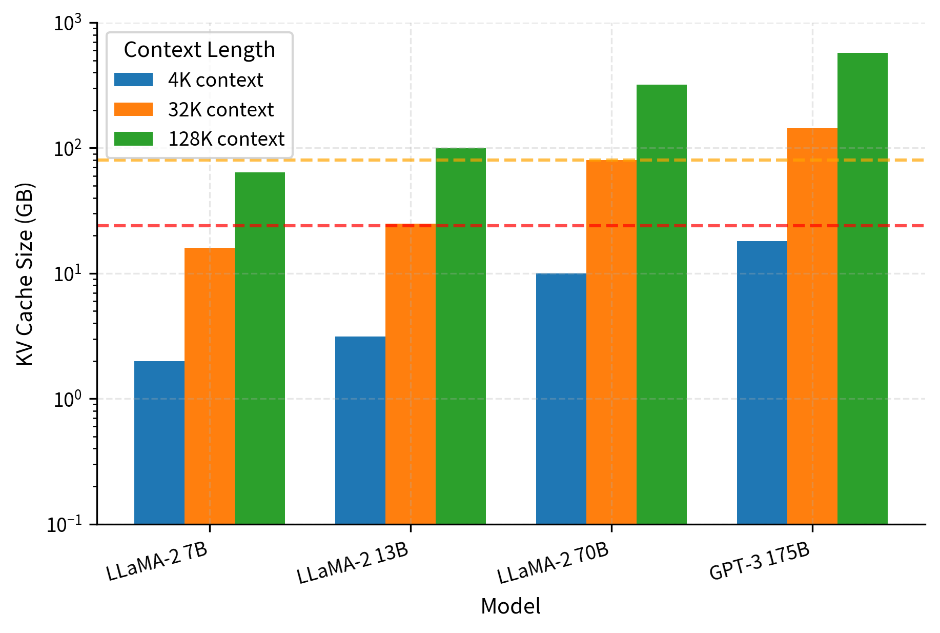
This memory pressure is the driving motivation behind MQA. When the cache alone exceeds available GPU memory, you can't run inference at all, regardless of how fast your hardware is.
Multi-Query Attention: Extreme Sharing
Multi-Query Attention, introduced by Noam Shazeer in 2019, addresses the KV cache problem through aggressive parameter sharing. The core insight is simple: instead of having separate key and value projections (one per head), use just one shared key and one shared value projection across all heads.
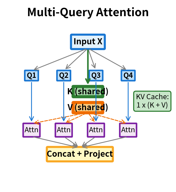
Multi-Query Attention maintains multiple query heads but shares a single key head and a single value head across all of them. Each query head computes attention using the same keys and values, reducing the KV cache size by a factor of (the number of heads).
The MQA Formulation
To truly understand Multi-Query Attention, we need to first build intuition about what multi-head attention actually does and why each component exists. Think of attention as a retrieval system: queries ask questions, keys advertise what information is available, and values contain the actual content to retrieve. Multi-head attention runs multiple such retrieval systems in parallel, each learning to find different kinds of relationships.
Step 1: The Standard Multi-Head Attention Baseline
In standard multi-head attention, each head transforms the input through its own learned projection matrices. Given an input sequence , we compute head-specific queries, keys, and values:
where:
- : the input sequence with tokens, each represented as a -dimensional vector
- : the query projection matrix for head
- : the key projection matrix for head
- : the value projection matrix for head
- : the dimension of queries and keys per head (typically )
- : the dimension of values per head (often equal to )
The subscript on each projection matrix is the key detail here. It tells us that every head learns its own transformation. Head 1 might learn to project tokens in a way that emphasizes syntactic features, while head 2 might emphasize semantic similarity. This specialization is what makes multi-head attention so powerful: the model can simultaneously attend to different types of relationships.
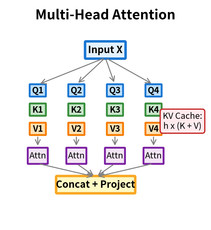
But this flexibility comes at a cost. During inference, we must cache the keys and values for each head separately. With 32 heads, we store 32 different matrices and 32 different matrices. This is where the memory bottleneck arises.
Step 2: The MQA Insight: Sharing Keys and Values
MQA asks a provocative question: do we really need different keys and values for each head? The hypothesis is that while different heads benefit from asking different questions (different queries), they might be able to share a common "index" (keys) and "content store" (values).
Mathematically, MQA removes the subscript from the key and value projections:
Notice the key change:
- : still has subscript , meaning each head retains its own query projection
- and : no subscript, meaning a single projection shared across all heads
The resulting matrices have dimensions:
- : unique query matrix for head
- : one shared key matrix for all heads
- : one shared value matrix for all heads
This is a simple but effective change. Different heads can still "ask different questions" because each projects the input into its own query space. But they all look up answers from the same key-value store. It's like having 32 researchers who each have their own research questions but share access to a single library catalog and book collection.
Step 3: Computing Attention with Shared KV
Each head now computes attention using its unique queries against the shared keys and values:
Let's trace through what happens in this formula:
-
Compute attention scores: produces an matrix where entry measures how much token at position should attend to position . Because is unique to head , each head produces different attention patterns.
-
Scale the scores: Dividing by prevents the dot products from growing too large as dimension increases. Without scaling, the softmax would produce very peaked distributions, making gradients vanish during training.
-
Normalize to weights: The softmax converts each row of scores into a probability distribution that sums to 1. These are the attention weights.
-
Aggregate values: Multiplying by computes a weighted sum of value vectors. All heads aggregate from the same , but with different weights.
The key insight is that expressiveness comes from two sources: the diversity of attention patterns (which heads preserve through unique queries) and the diversity of retrieved content (which MQA sacrifices through shared values). Empirically, the diversity of attention patterns matters more than the diversity of values for most tasks.
To illustrate this, let's visualize how different query heads can produce distinct attention patterns even when sharing the same keys and values.
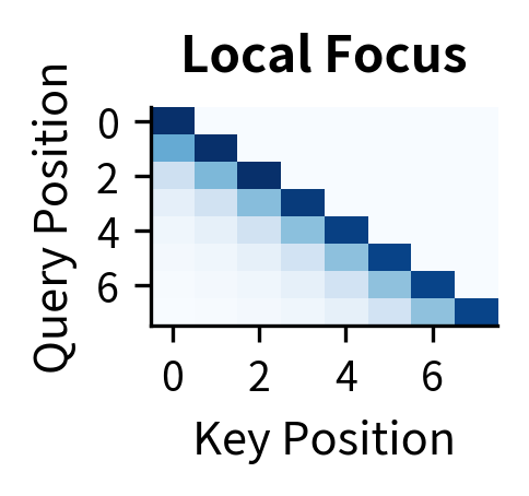

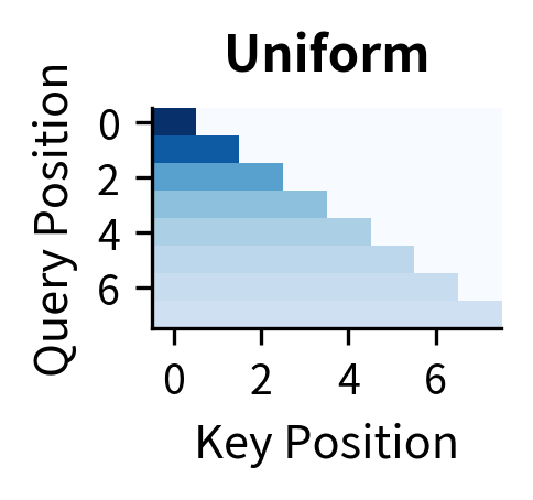
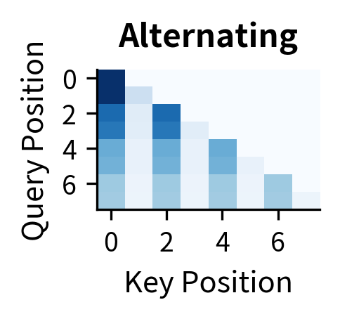
Each head learns a different way to "ask questions" of the shared key-value store. Head 1 might focus on recent context for local coherence, Head 2 might anchor to the beginning of the sequence, Head 3 might aggregate broadly, and Head 4 might pick up periodic patterns. The shared keys and values don't limit this diversity; they simply mean all heads retrieve from the same "library."
Step 4: Combining Head Outputs
Finally, we concatenate all head outputs and project back to the model dimension:
where:
- : the output from attention head , containing each head's weighted aggregation
- : concatenation along the feature dimension
- : the output projection that mixes information across heads
- : the total number of attention heads
This final projection is unchanged from standard MHA. Each head contributes its perspective, and the output projection learns to combine them into a coherent representation. The key benefit of MQA is that we achieve this with much less memory overhead during inference.
Visualizing the Difference
The architectural difference between MHA and MQA becomes clear when we visualize the projection structure.
Implementing Multi-Query Attention
Now that we understand the mathematical formulation, let's translate it into working code. The implementation will reveal exactly how the parameter sharing manifests in practice and why it leads to such significant memory savings.
We'll build MQA from scratch, examining each component to understand how it differs from standard multi-head attention. By the end, you'll see that the core change is just a matter of adjusting projection dimensions.
The Core MQA Module
The main difference between MHA and MQA lies in the output dimensions of the projection layers. In MHA, the key and value projections output num_heads * head_dim dimensions (one set of K/V vectors per head). In MQA, they output just head_dim (a single set of K/V vectors shared across all heads).
Let's implement this step by step, with comments highlighting the critical differences.
Several implementation details deserve attention:
Projection dimensions: The query projection outputs num_heads * head_dim dimensions because each head needs its own query vectors. But the key and value projections output only head_dim, producing a single set of K/V vectors. This is the source of our memory savings.
Broadcasting: When we compute torch.matmul(q, k.transpose(-2, -1)), PyTorch's broadcasting rules handle the dimension mismatch. The query tensor has shape (batch, num_heads, seq, head_dim) while the key tensor has shape (batch, 1, seq, head_dim). Broadcasting automatically replicates the single key across all heads, computing the correct attention scores without physically copying the data.
KV cache handling: The cache stores only the shared K and V tensors, not per-head copies. When we concatenate past keys with new keys, we're working with tensors of shape (batch, 1, seq, head_dim) rather than (batch, num_heads, seq, head_dim). This is where the memory reduction materializes during autoregressive generation.
Comparing Parameter Counts
To make the savings concrete, let's count parameters in MHA versus MQA for a realistic configuration.
The numbers reveal the trade-off clearly. MQA reduces the K and V projection parameters by exactly num_heads (32x in this case). However, the total attention layer parameter reduction is more modest, around 50%, because the query and output projections remain unchanged at full size.
This distinction matters: the parameter savings affect model size and training memory, but the real win comes during inference. The KV cache stores the outputs of the K and V projections, not the projection matrices themselves. Since each forward pass produces only one K vector and one V vector per token (instead of 32), the cache reduction matches the full 32x factor. This is why MQA changes the economics of inference even though its impact on total parameter count is more modest.
MQA Memory Benefits
MQA's main benefit appears during inference. The KV cache reduction is proportional to the number of heads, which can be substantial for modern large models.
Calculating KV Cache Savings
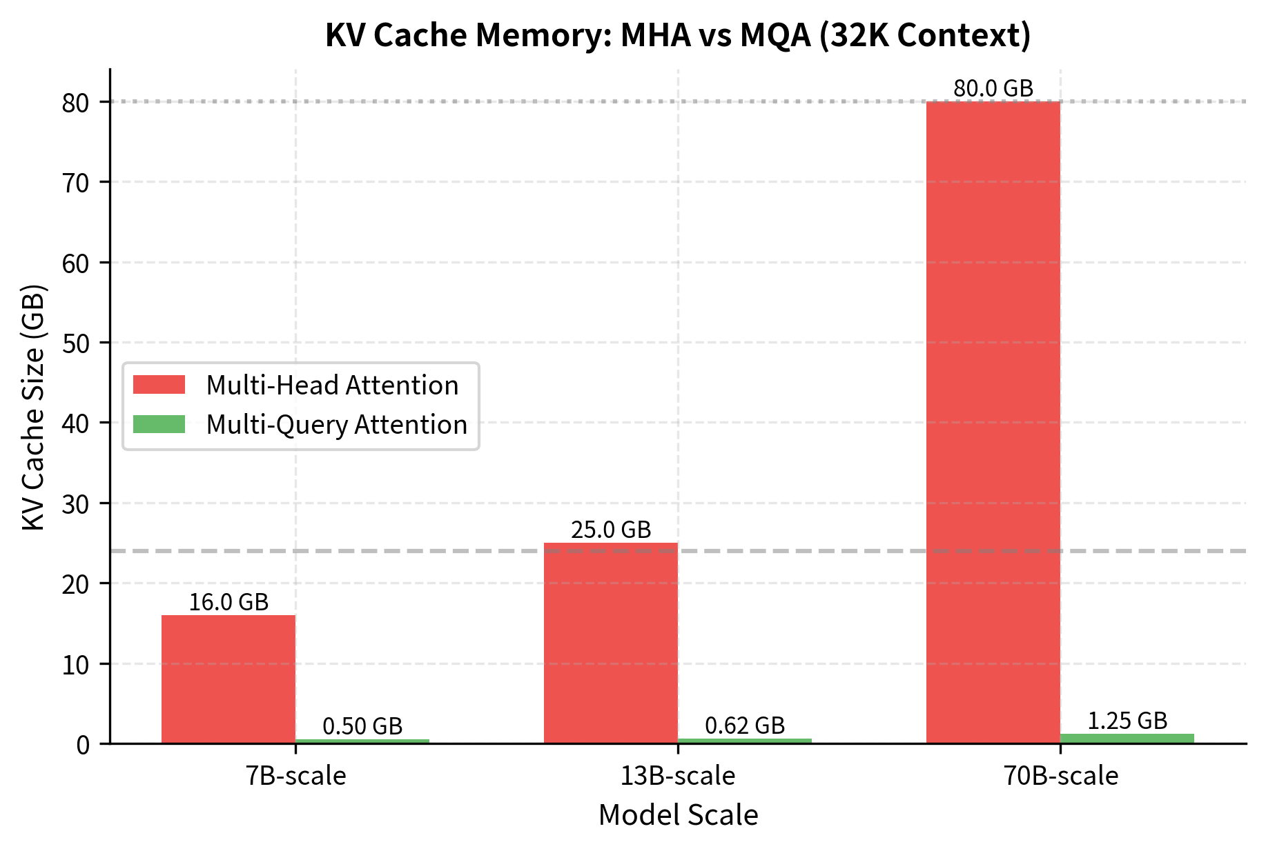
The table shows that the cache reduction factor exactly matches the number of attention heads. For the 7B-scale model with 32 heads, MQA reduces the cache from 8 GB to 0.25 GB. The 70B-scale model with 64 heads drops from 40 GB to just 0.625 GB. These reductions determine whether inference is feasible on given hardware.
The cache reduction factor equals the number of attention heads. A 7B model with 32 heads sees its cache shrink from 8 GB to 0.25 GB, while a 70B model with 64 heads drops from 40 GB to under 1 GB. This is the difference between requiring a cluster of GPUs and running inference on a single consumer card.
The scaling behavior becomes even clearer when we plot cache growth as a function of context length.
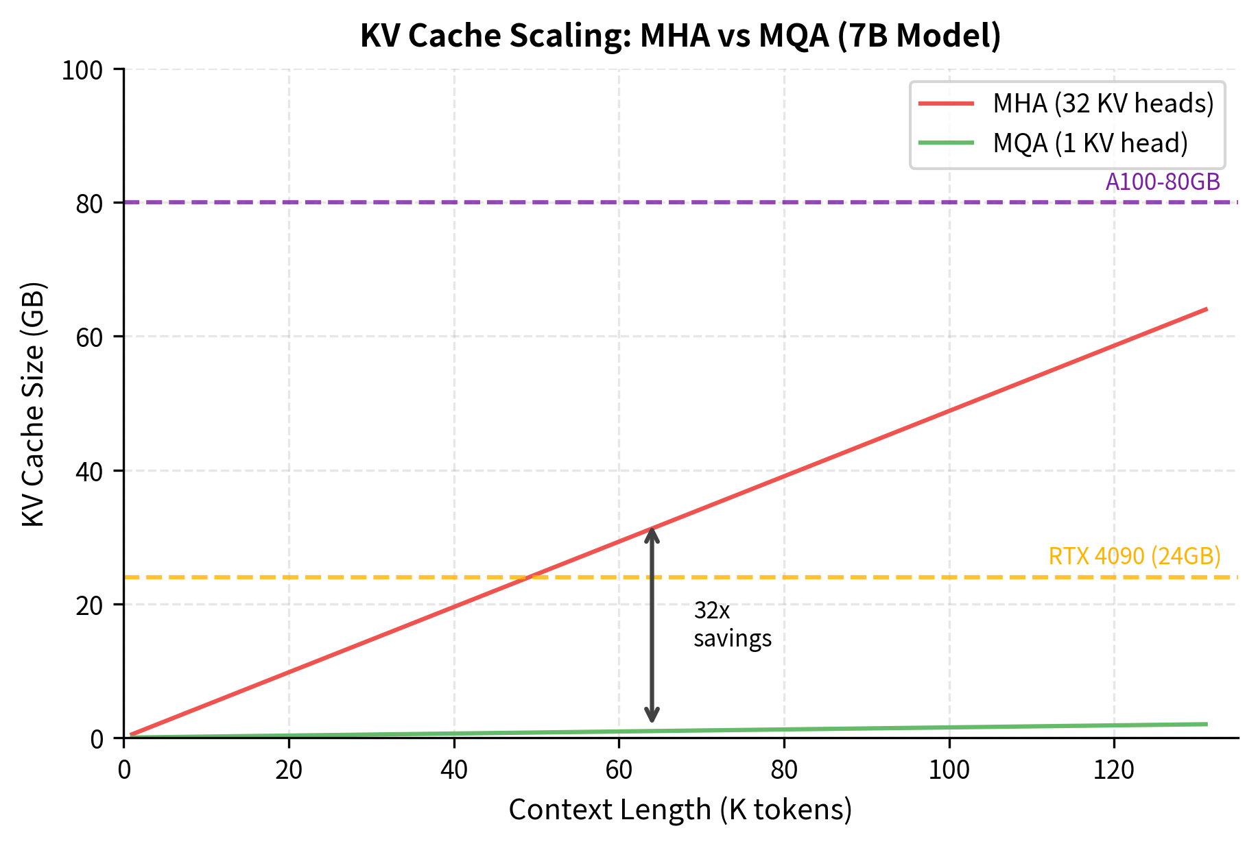
The linear relationship between context length and cache size explains why long-context models are so memory-hungry. At 128K tokens, the MHA cache alone requires 32 GB, which exceeds the memory of most consumer GPUs before we even load the model weights. MQA brings this down to 1 GB, making long-context inference practical on a single GPU.
Throughput Implications
The memory savings translate directly into throughput improvements. With less memory consumed by the KV cache, you can:
- Serve longer contexts: Fit 128K tokens instead of 8K on the same hardware
- Increase batch sizes: Process more requests in parallel
- Reduce hardware costs: Serve the same load with fewer GPUs
At 64K context, MHA can only serve 1 request at a time, while MQA can batch 32+ requests. This translates to significant throughput improvements in production settings.
The following heatmap visualizes the feasible operating space for both architectures. Each cell shows whether a given batch size and context length combination fits within GPU memory.
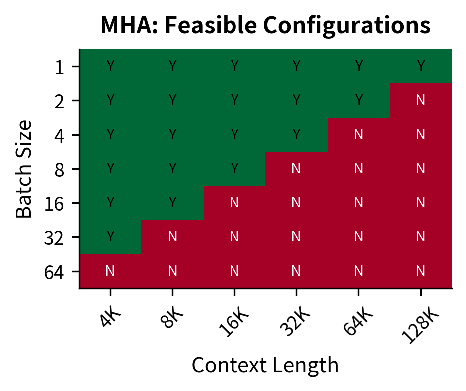
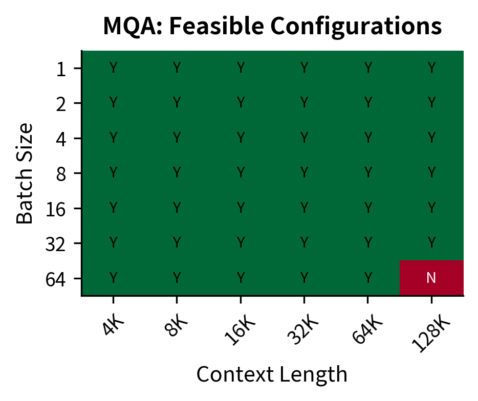
The difference is clear. With MHA, the A100-80GB can only handle batch size 1 beyond 32K context, and batch size 4 is already impossible at 16K. With MQA, you can run batch size 64 at 32K context, or batch size 16 even at 128K. This expanded operating space translates directly to higher throughput and better hardware utilization.
Quality Trade-offs
The extreme parameter sharing in MQA raises an important question: what do we lose by sharing keys and values across all heads? The answer is nuanced and depends on the task.
What Each Head Learns
In standard MHA, each head can specialize its key and value representations. Research has shown that different heads often capture distinct linguistic phenomena:
- Syntactic heads: Attend to grammatical structure (subject-verb, modifier-noun)
- Semantic heads: Capture meaning relationships (synonymy, entailment)
- Positional heads: Focus on local context or specific positions
- Rare pattern heads: Specialize in infrequent but important patterns
When we share K and V, all heads must use the same "retrieval index" (keys) and the same "information content" (values). They can still differ in what they query for (different Q projections), but they're constrained to retrieve from the same representation.
Empirical Quality Results
The original MQA paper and subsequent studies found modest quality degradation. Let's examine representative benchmark results across translation, summarization, and language modeling tasks.
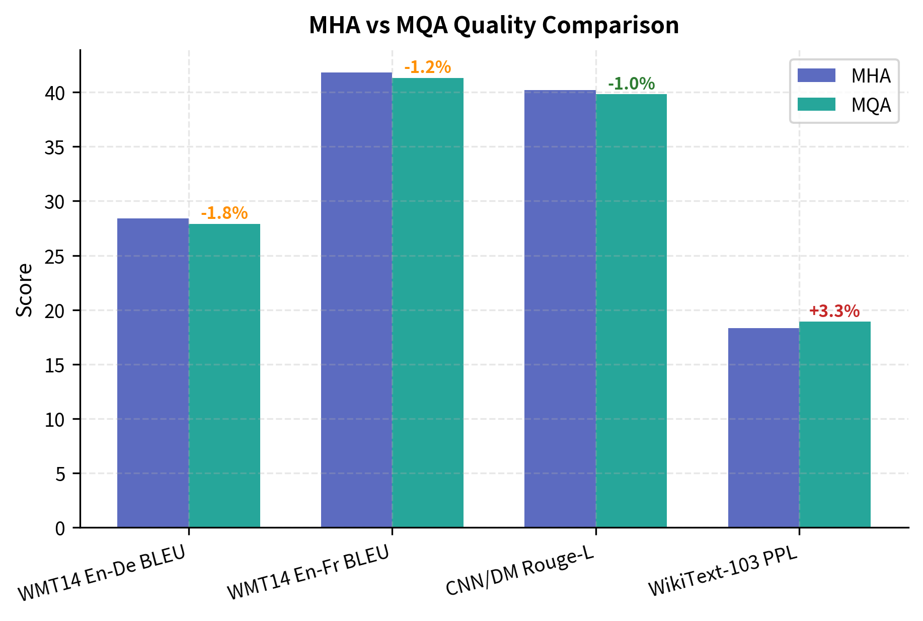
The quality degradation typically falls in the 1-3% range. For many applications, especially inference-heavy deployments where throughput matters more than the last percentage point of accuracy, this is an excellent trade-off.
When MQA Hurts More
Some tasks are more sensitive to the reduced expressiveness:
- Long-range reasoning: Tasks requiring diverse attention patterns over long contexts
- Multi-task learning: Models expected to handle many different tasks
- Fine-grained linguistic tasks: Parsing, detailed entity typing, relation extraction
For these applications, Grouped Query Attention (GQA) offers a middle ground, sharing K/V among groups of heads rather than all heads.
MQA vs GQA
Grouped Query Attention interpolates between MHA and MQA by grouping heads and sharing K/V within each group.
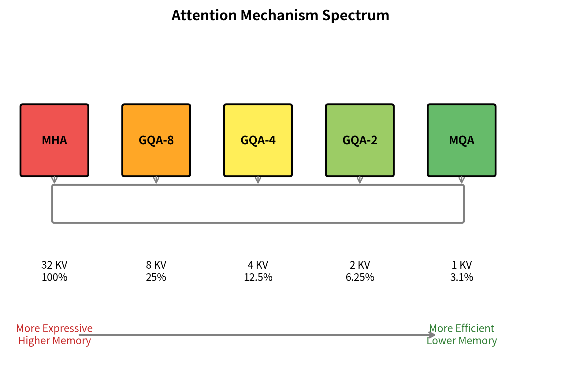
The spectrum shows a smooth trade-off between expressiveness and efficiency. GQA-8 with 8 KV heads provides a 4x cache reduction while maintaining most of the representational power of full MHA. GQA-4 doubles the savings to 8x. MQA represents the extreme endpoint with maximum savings but minimum KV diversity.
Why GQA Often Wins
In practice, GQA with 4-8 KV heads often provides the best trade-off:
- Near-MQA memory efficiency: 4-8x cache reduction covers most memory constraints
- Near-MHA quality: Multiple KV representations preserve expressiveness for complex tasks
- Flexible tuning: Choose the balance point appropriate for your deployment
LLaMA-2 70B uses GQA with 8 KV heads (sharing among 8 query heads each), achieving excellent quality while maintaining reasonable inference costs. Mistral and many other modern models follow similar patterns.
Practical Implementation Considerations
Converting MHA to MQA
If you have a pre-trained MHA model and want MQA's efficiency gains, you can convert it through careful weight averaging:
The conversion uses averaging, which works reasonably well but may require fine-tuning to recover any lost quality. Research suggests that a small amount of fine-tuning (1-5% of original training) can recover most of the original model's performance.
Uptraining for Better Quality
Rather than training from scratch with MQA, many practitioners start with MHA pre-training and then "uptrain" to MQA or GQA:
- Pre-train with MHA: Full expressiveness during the learning phase
- Convert to MQA/GQA: Average or group the KV projections
- Fine-tune briefly: Recover quality with the new architecture
- Deploy efficiently: Enjoy the memory benefits during inference
This approach often yields better results than training MQA from scratch, as the model benefits from the full representational capacity during the critical pre-training phase.
Summary
Multi-Query Attention addresses a key bottleneck in large language model deployment: KV cache memory consumption. By sharing a single key and value projection across all attention heads, MQA achieves substantial memory reductions:
- Memory reduction: KV cache shrinks by a factor of (the number of heads), often 32-64x for modern models
- Throughput gains: Smaller caches enable larger batch sizes and longer contexts on the same hardware
- Modest quality loss: Typically 1-3% degradation on standard benchmarks
- Parameter savings: K and V projection parameters reduce by a factor of
The trade-off between efficiency and expressiveness has led to the popular Grouped Query Attention (GQA), which shares K/V among groups of heads rather than all heads. Most modern LLMs, including LLaMA-2, Mistral, and others, use GQA with 4-8 KV heads as a practical middle ground.
For inference-heavy deployments where throughput matters more than the last percentage point of accuracy, MQA and GQA are essential techniques. They transform the economics of serving large language models, making long-context generation feasible on hardware that would otherwise be memory-bound.
Key Parameters
When implementing or configuring MQA and GQA, these parameters have the greatest impact on the memory-quality trade-off:
- num_heads (
int): The number of query heads. This determines model expressiveness and directly affects the cache reduction factor when using MQA. Typical values range from 32 (7B models) to 128 (largest models). - num_kv_heads (
int): The number of key-value heads. Set to 1 for MQA, equal tonum_headsfor standard MHA, or an intermediate value for GQA. Common GQA configurations use 4-8 KV heads regardless of query head count. - head_dim (
int): The dimension of each attention head. Standard values are 64 or 128. Larger head dimensions increase per-token cache size but may improve attention quality. Most modern LLMs use 128. - hidden_size (
int): The model's hidden dimension, typically equal tonum_heads * head_dim. This determines the size of projection matrices and overall model capacity.
When choosing between MHA, GQA, and MQA, consider your deployment constraints. If memory is severely limited or batch sizes must be large, MQA provides maximum savings. If quality is the priority and memory is less constrained, GQA with 4-8 KV heads offers a balanced approach that most production systems favor.
Quiz
Ready to test your understanding? Take this quick quiz to reinforce what you've learned about Multi-Query Attention and its memory efficiency trade-offs.

Comments