

Learn how temperature scaling reshapes probability distributions during text generation, with mathematical foundations, implementation details, and practical guidelines for selecting optimal temperature values.

This article is part of the free-to-read Language AI Handbook
Choose your expertise level to adjust how many terms are explained. Beginners see more tooltips, experts see fewer to maintain reading flow. Hover over underlined terms for instant definitions.
execute: cache: true jupyter: python3
Decoding Temperature
When a language model predicts the next token, it outputs a probability distribution over its entire vocabulary. Given the prompt "The capital of France is," the model might assign 0.85 to "Paris," 0.05 to "Lyon," 0.02 to "Marseille," and tiny probabilities to thousands of other tokens. Temperature is the parameter that controls how we interpret and sample from this distribution.
At its core, temperature answers a fundamental question: how much should we trust the model's probability rankings? A temperature of 1.0 preserves the learned distribution exactly. Lower temperatures sharpen the distribution, making high-probability tokens even more likely and pushing the model toward deterministic, predictable output. Higher temperatures flatten the distribution, giving lower-probability tokens a fighting chance and introducing creative variability.
This chapter explores temperature from first principles. You'll learn the mathematical mechanics of temperature scaling, visualize how it reshapes probability distributions, implement temperature-controlled sampling, and develop intuition for selecting appropriate values across different generation tasks.
How Temperature Scaling Works
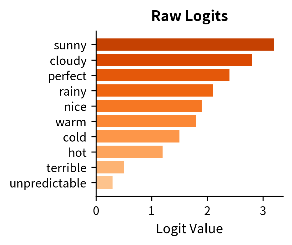
To understand temperature, we need to start with what language models actually output. When you feed a prompt into a model, the final layer doesn't produce probabilities directly. Instead, it outputs a vector of logits: raw, unbounded scores for every token in the vocabulary. A logit of 5.0 doesn't mean "5% probability." It's just a score indicating relative preference. The token with the highest logit is the model's top choice, but we need a way to convert these scores into actual probabilities we can sample from.
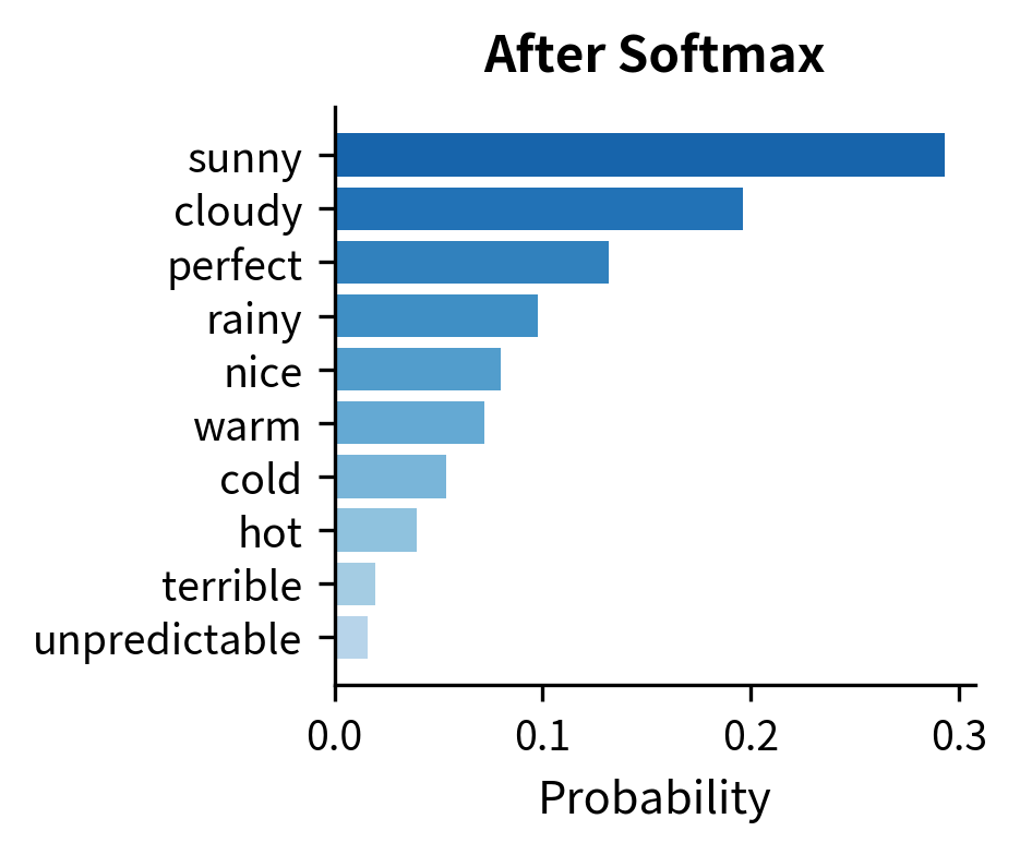
This is where the softmax function enters the picture. Softmax takes a vector of arbitrary real numbers and transforms them into a valid probability distribution: all values become positive and sum to 1. For a vocabulary of tokens with logits , the standard softmax computes:
where:
- : the logit for token , which can be any real number
- : the exponential function applied to the logit, ensuring the result is positive
- : the sum of all exponentiated logits, serving as a normalizing constant
The exponential function is crucial here. It preserves the ordering of logits (higher logits still get higher probabilities) while ensuring all outputs are positive. The denominator normalizes everything to sum to 1.
But here's the problem: the standard softmax gives us exactly one distribution. What if we want more control? What if the model's top choice is good but we want to explore alternatives? Or conversely, what if we want to make the model more decisive, committing more strongly to its best guess?
Introducing the Temperature Parameter
Temperature gives us that control. The idea is elegantly simple: before applying softmax, we divide all logits by a temperature parameter . This single modification lets us reshape the entire probability distribution.
Temperature scaling divides the logits by a temperature parameter before computing the softmax. Given logits for vocabulary token , the temperature-scaled probability is:
where:
- : the logit (raw score) for token output by the model's final layer
- : the temperature parameter, a positive scalar that controls distribution sharpness
- : the exponential of the scaled logit, which ensures positive values
- : the sum over all tokens in the vocabulary, serving as a normalizing constant
When , this reduces to the standard softmax. When , dividing by a fraction amplifies the logit differences. When , dividing by a larger number compresses the differences.
The name "temperature" comes from statistical mechanics, where a similar parameter controls the randomness of particle states in a physical system. At low temperature, particles settle into their lowest-energy states (highly ordered). At high temperature, particles explore many states more freely (more disordered). The analogy carries over perfectly to language models: low temperature means the model commits to its top choices; high temperature means it explores more freely across the vocabulary.
A Concrete Example: Three Candidate Tokens
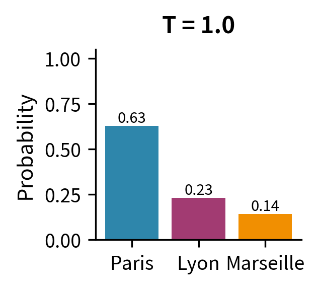
Let's make this concrete. Suppose a language model is completing the prompt "The capital of France is" and has narrowed down to three plausible tokens: "Paris," "Lyon," and "Marseille." The model outputs logits of 2.0, 1.0, and 0.5 respectively. Paris has the highest logit, so it's the model's top choice, but how do the probabilities change as we vary temperature?
The results reveal temperature's effect clearly. At , "Paris" dominates with 84.4% probability, leaving only scraps for the alternatives. The model is highly confident, almost deterministic. At (standard softmax), we get the baseline distribution: Paris at 59%, Lyon at 22%, Marseille at 13%. The model still prefers Paris but gives meaningful weight to alternatives. At , the distribution flattens dramatically: Paris drops to 39%, and even Marseille climbs to 22%. The model is now much more willing to sample less-preferred tokens.
The Mathematics of Sharpening and Flattening
Why does this simple division produce such dramatic effects? The key insight comes from examining how temperature affects the probability ratio between any two tokens. Understanding this ratio reveals the core mechanism.
Consider two tokens with logits and , where (token 1 is preferred). Under temperature scaling, their probabilities are:
When we compute the ratio , something beautiful happens: the normalization constants cancel out completely:
where:
- : the logit gap between the two tokens, representing how much more the model prefers token 1
- : temperature, which scales how strongly this preference translates to probability
- : the exponential function, which converts the scaled difference to a multiplicative ratio
This formula is the key to understanding temperature. The effective logit gap becomes . Temperature acts as a divisor on the gap itself, not on the probabilities directly.
When , we divide the gap by a fraction, which amplifies it. A logit difference of 1.0 at becomes an effective difference of . The exponential of 2.0 is about 7.4, so the preferred token becomes 7.4 times more likely than its competitor. The distribution sharpens.
When , we divide the gap by a number greater than 1, which compresses it. The same logit difference of 1.0 at becomes an effective difference of . The exponential of 0.5 is about 1.65, so the preferred token is only 1.65 times more likely. The distribution flattens.
Let's verify this with actual calculations:
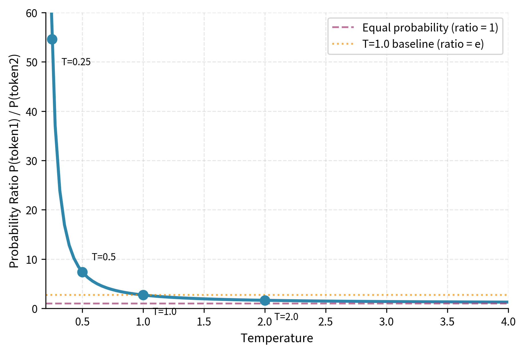
The numbers tell the story. At , the higher-probability token is 55 times more likely than its competitor, an overwhelming advantage. At (baseline), the ratio is 2.72 (which is just ). At , that ratio shrinks to just 1.28, meaning the two tokens are nearly equally likely despite the original logit gap. Temperature truly acts as a dial between certainty and randomness.
Temperature Extremes: The Limiting Cases
To build complete intuition, consider what happens at the mathematical extremes:
As (approaching zero):
The effective logit gap grows without bound for any non-zero gap. The exponential of infinity is infinity, so the probability ratio between the top token and any other token becomes infinite. In practice, this means all probability mass concentrates on the single highest-logit token. This limiting case is equivalent to greedy decoding or argmax selection: always pick the most likely token, with zero randomness.
As (approaching infinity):
The effective logit gap shrinks toward zero for any finite gap. The exponential of zero is 1, so the probability ratio between any two tokens approaches 1:1. All tokens become equally likely regardless of their original logits. The distribution approaches uniform, and generation becomes pure random sampling from the vocabulary.
Neither extreme is useful for text generation. produces repetitive, predictable text that lacks nuance. The model keeps selecting the same high-probability continuations, often getting stuck in loops. produces incoherent gibberish since token selection ignores the model's learned preferences entirely. Practical values fall between these extremes, typically in the range 0.1 to 2.0.
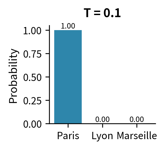
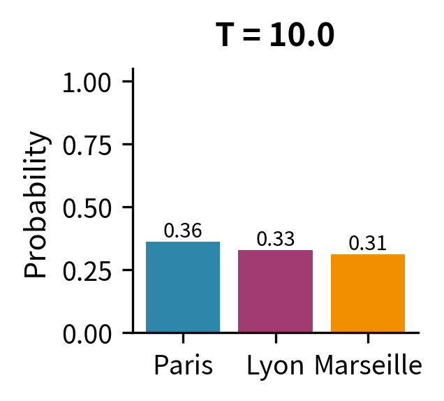
The visualization makes the extremes visceral. At , Paris captures 99.3% of the probability mass, leaving virtually nothing for alternatives. At , the three tokens have nearly equal probability (35%, 33%, 32%), approaching the uniform distribution of 33.3% each. The standard softmax at sits in between, reflecting the model's learned preferences while still allowing meaningful sampling diversity.
Visualizing Temperature Effects
To develop intuition for temperature, let's visualize how it reshapes a realistic probability distribution. We'll simulate logits from a language model predicting the next token after "The weather today is" and examine distributions across a range of temperatures.
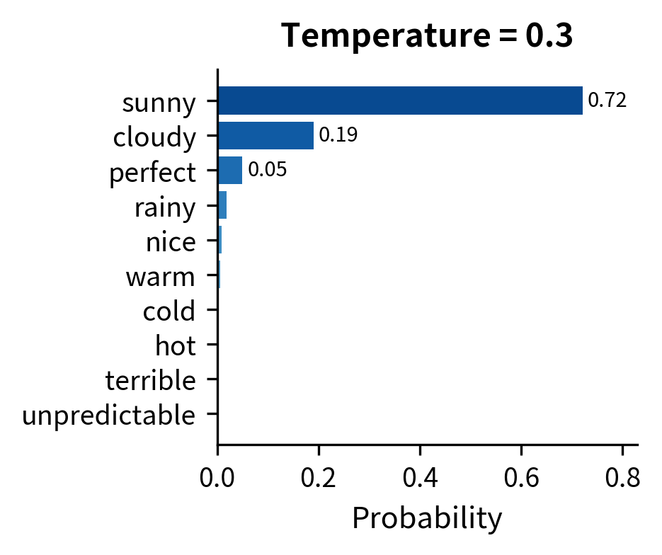
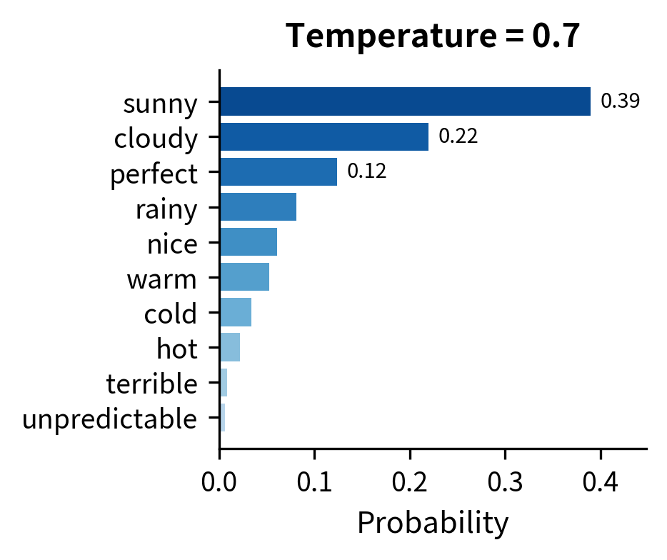
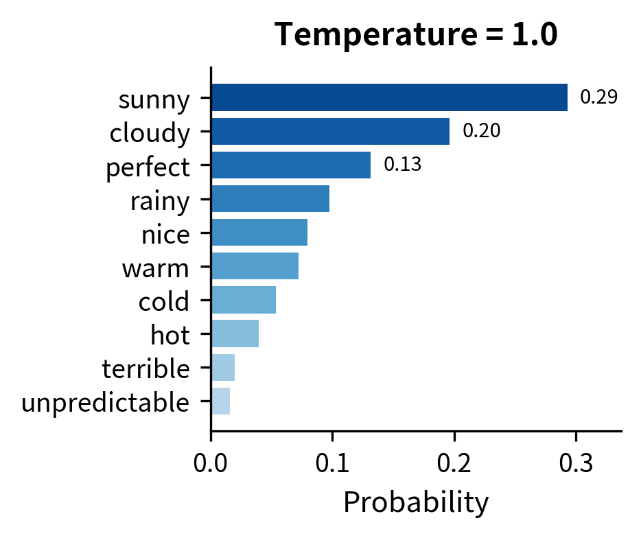
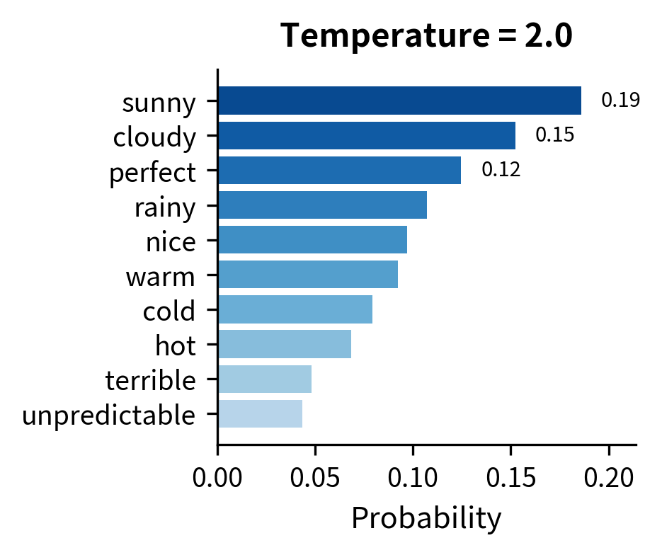
At , "sunny" captures over 60% probability, leaving little room for alternatives. This produces predictable text but misses the natural variation in language. At , the top five tokens each have between 10% and 18% probability. Sampling here introduces meaningful diversity while still favoring contextually appropriate completions.
A heatmap reveals the continuous transformation more clearly. Each row shows one token's probability as temperature varies from left (low T, sharp distribution) to right (high T, flat distribution):
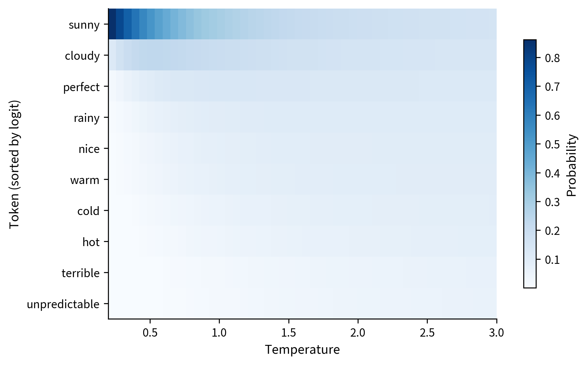
The heatmap shows the redistribution of probability mass. At low temperature, the top token ("sunny") absorbs most probability (dark band at top-left). As temperature increases, probability spreads more evenly across all tokens (lighter, more uniform coloring toward the right). The transition isn't abrupt but smooth and continuous.
Entropy and Temperature
Entropy quantifies the uncertainty or "spread" of a probability distribution. For a discrete distribution over tokens, Shannon entropy is defined as:
where:
- : the entropy of distribution , measured in bits
- : the probability of token
- : logarithm base 2, so entropy is measured in bits
- The negative sign ensures entropy is positive (since of a probability is negative)
Entropy has intuitive extremes. When one token has probability 1.0 and all others have 0, entropy equals 0 bits, meaning there's no uncertainty. When all tokens are equally likely with probability , entropy reaches its maximum of bits.
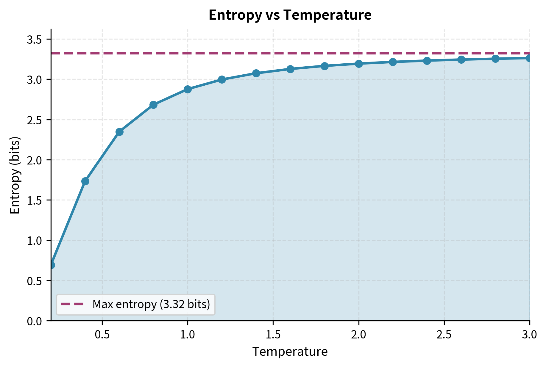
Temperature directly controls entropy. Low temperature concentrates probability mass on high-logit tokens, reducing entropy. High temperature spreads probability more evenly, increasing entropy toward the maximum.
With 10 tokens in our vocabulary, maximum entropy (achieved when the distribution is uniform) is bits. At , entropy drops to around 1.5 bits, indicating the distribution is highly concentrated on just a few tokens. At , entropy approaches 3 bits, nearly matching the uniform distribution's maximum uncertainty.
Implementing Temperature-Controlled Sampling
Let's build a complete temperature sampling implementation. We'll start with a function that samples from temperature-scaled logits, then extend it to generate token sequences.
The function handles the edge case of by returning the argmax (greedy decoding). For positive temperatures, it scales logits, converts to probabilities, and samples using PyTorch's multinomial function.
The empirical frequencies closely match the theoretical probabilities computed earlier. At , samples cluster heavily on "sunny" and "cloudy." At , we see meaningful representation from lower-probability tokens like "warm," "nice," and "cold."
Batch Sampling for Efficiency
In practice, we often want to generate multiple completions or compare outputs across temperatures. Here's a vectorized implementation:
At low temperature, we see repeated "sunny" selections. Higher temperatures introduce variety, sometimes surfacing less expected but still contextually reasonable tokens.
Temperature Selection Guidelines
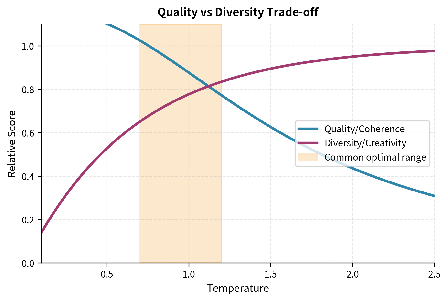
Choosing the right temperature depends on your application. The key insight is that temperature controls the trade-off between coherence and creativity. Lower temperatures produce safer, more predictable text. Higher temperatures introduce novelty but risk incoherence.
Task-Based Recommendations
Different generation tasks call for different temperature settings:
| Task | Recommended T | Rationale |
|---|---|---|
| Code generation | 0.0 - 0.3 | Correctness matters; creativity can introduce bugs |
| Factual Q&A | 0.0 - 0.5 | Accuracy over variety; want the most likely correct answer |
| Translation | 0.3 - 0.7 | Balance fluency with fidelity to source meaning |
| Creative writing | 0.7 - 1.2 | Encourage unexpected but coherent word choices |
| Brainstorming | 1.0 - 1.5 | Explore diverse ideas; some randomness is beneficial |
| Poetry/experimental | 1.2 - 2.0 | Prioritize novelty and surprise |
For code and factual tasks, you often want temperature near zero. A slight temperature (0.1-0.2) can prevent the model from getting stuck in repetitive loops while still strongly favoring high-probability outputs. For creative tasks, temperatures between 0.7 and 1.2 typically produce the best balance of quality and variety.
The Quality-Diversity Trade-off
Temperature creates an inherent trade-off. As you increase temperature, you gain:
- Lexical diversity: More varied word choices, less repetition
- Idea exploration: Access to less probable but potentially interesting continuations
- Reduced mode collapse: Less tendency to repeat the same phrases
But you also risk:
- Coherence degradation: Sentences that don't follow logically
- Factual errors: Lower-probability (and potentially wrong) claims
- Grammatical mistakes: Unusual token sequences that violate syntax
The sweet spot depends on how much you value diversity versus correctness. For a customer service chatbot, coherence and accuracy dominate: use low temperature. For a creative writing assistant, moderate temperature encourages the unexpected turns that make prose interesting.
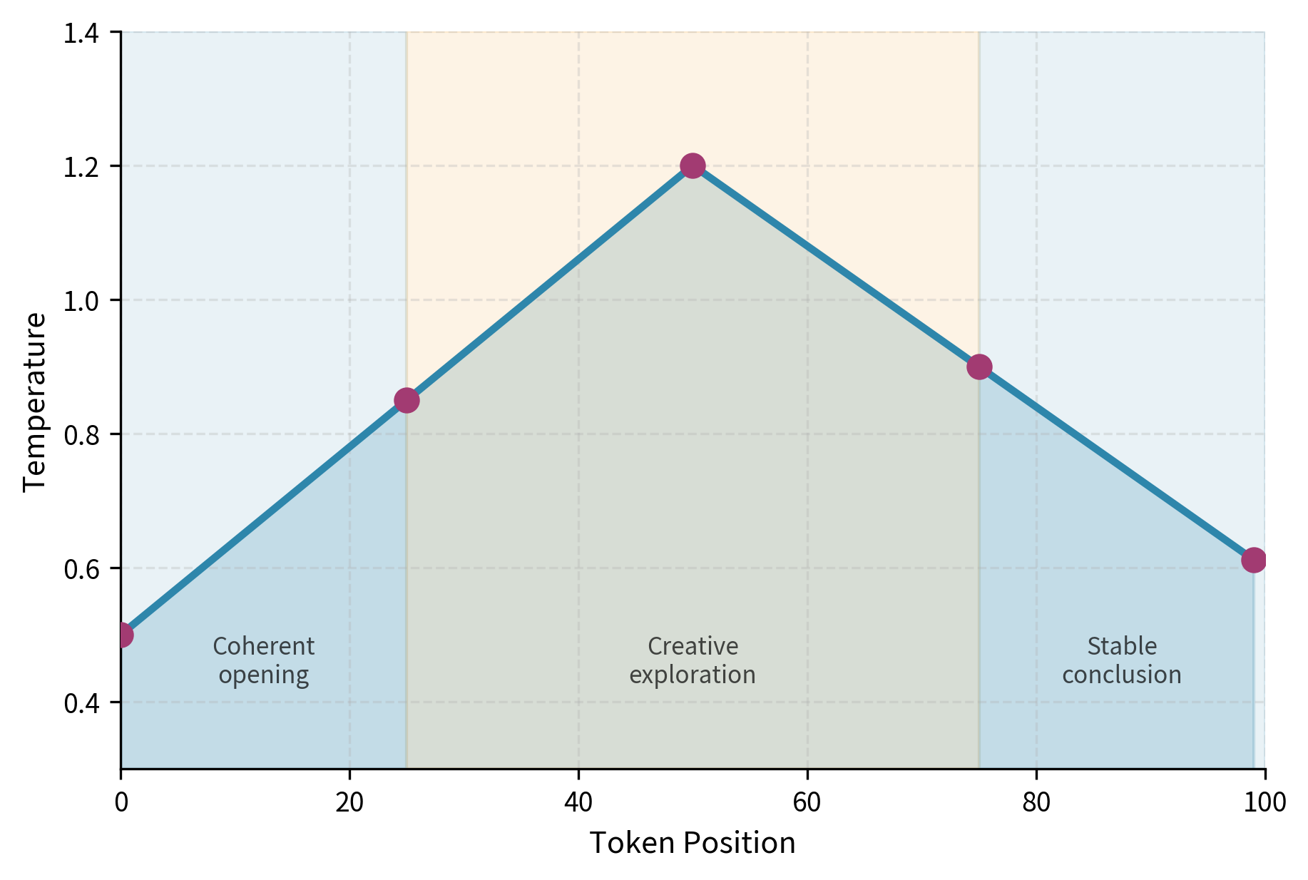
Dynamic Temperature
Some applications benefit from varying temperature during generation. You might start with low temperature to establish a coherent beginning, then increase temperature to introduce variation, then decrease again to conclude coherently. This technique requires careful tuning but can produce text that is both well-structured and creatively varied.
Worked Example: Generating Text Completions
Let's put temperature into practice with a complete text generation example. We'll use a small GPT-2 model to generate completions at different temperatures and observe the output characteristics.
Now let's generate completions for a prompt at different temperatures:
At , the model produces focused, predictable continuations. At , we see more varied vocabulary while maintaining coherence. At , creativity increases but the text may occasionally veer into unusual territory.
Comparing Multiple Samples
One sample doesn't reveal the full picture. Let's generate multiple completions at each temperature to see the distribution of outputs:
At , the four samples likely share similar themes and phrasing. At , you'll observe more divergent narratives and word choices.
Measuring Output Diversity
We can quantify diversity by measuring how different the generated samples are from each other. One simple metric is the number of unique n-grams across samples:
Higher temperatures produce higher diversity ratios, confirming that the outputs explore a broader range of vocabulary and phrases.
Limitations and Impact
Temperature is powerful but imperfect. It operates on the entire vocabulary uniformly, which can cause problems when you want to encourage diversity in some dimensions but not others.
The fundamental limitation is that temperature is a single scalar applied to all logits equally. Consider a medical question-answering system where you want diverse phrasing (how the answer is expressed) but not diverse facts (what claims are made). Temperature cannot distinguish between these: raising temperature increases variety in both phrasing and factual content. This creates a real tension in domains where accuracy matters but repetitive outputs frustrate users.
Temperature also interacts poorly with very long generation. Early tokens sampled at high temperature can push the model into unfamiliar territory, leading to compounding errors as generation proceeds. A single unusual word choice in token 5 might make token 50 completely incoherent. This is why many practitioners combine temperature with other techniques like top-k or nucleus sampling (covered in the next chapters) to constrain the damage from high-temperature sampling.
Despite these limitations, temperature fundamentally shaped how we interact with language models. Before temperature scaling became standard, language model outputs felt robotic and predictable. Temperature gave users a dial to explore the space of possible outputs, making language models feel more creative and less deterministic. The concept transfers beyond language: temperature-like parameters appear in image generation, music synthesis, and other generative AI systems. The intuition that "higher temperature means more randomness" has become part of the basic vocabulary of generative AI.
The success of temperature scaling also revealed something important about language model training. The fact that simply rescaling logits produces coherent but varied outputs suggests that models learn meaningful probability distributions over vocabulary. The relative ordering of token probabilities carries semantic information: "sunny" really is more appropriate than "elephant" after "The weather today is," and temperature preserves this ordering while adjusting the degree of concentration.
Summary
Temperature controls the sharpness of the probability distribution during language model sampling. By dividing logits by a temperature parameter before softmax, we can make the distribution more peaked (low ) or more uniform (high ).
Key takeaways:
- preserves the learned distribution. Lower values sharpen it; higher values flatten it.
- approaches greedy decoding (argmax). approaches uniform random sampling.
- Practical ranges typically fall between 0.1 and 2.0, with most applications using 0.3 to 1.2.
- Task matters: Factual and code generation prefer low temperature. Creative writing benefits from higher values.
- Temperature controls the quality-diversity trade-off: more diversity comes at the cost of coherence.
- Temperature affects all tokens uniformly, which can be limiting when you want selective diversity.
Temperature is often combined with top-k and nucleus (top-p) sampling to get finer control over the output distribution. These techniques, covered in the following chapters, truncate the distribution before sampling, preventing temperature from giving meaningful probability to highly unlikely tokens.
Key Parameters
When implementing temperature-controlled sampling, these parameters determine behavior:
-
temperature(float, typically 0.1-2.0): The scaling factor applied to logits before softmax. Values below 1.0 sharpen the distribution, making high-probability tokens more dominant. Values above 1.0 flatten the distribution, giving lower-probability tokens more chance. A value of 1.0 preserves the original learned distribution. -
do_sample(bool): Whether to sample from the distribution (True) or use greedy decoding (False). Temperature only affects output whendo_sample=True. Withdo_sample=False, the model always selects the highest-probability token regardless of temperature. -
top_k(int, 0 to disable): When combined with temperature, restricts sampling to the top k most probable tokens. Settingtop_k=0disables this constraint, allowing temperature to affect the full vocabulary distribution. -
top_p(float, 0.0-1.0): Nucleus sampling threshold, often used alongside temperature. Settingtop_p=1.0disables nucleus sampling, isolating the temperature effect. Lower values restrict sampling to tokens whose cumulative probability reaches the threshold. -
max_new_tokens(int): Maximum number of tokens to generate. Longer sequences at high temperature tend to accumulate errors, so consider lower temperatures for longer outputs.
For most applications, start with temperature=0.7 and adjust based on output quality. Decrease if outputs are too random or incoherent; increase if outputs are too repetitive or predictable.
Quiz
Ready to test your understanding? Take this quick quiz to reinforce what you've learned about decoding temperature and probability distribution control.

Comments