

Master RNN architecture from recurrent connections to hidden state dynamics. Learn parameter sharing, sequence classification, generation, and implement an RNN from scratch.

This article is part of the free-to-read Language AI Handbook
Choose your expertise level to adjust how many terms are explained. Beginners see more tooltips, experts see fewer to maintain reading flow. Hover over underlined terms for instant definitions.
RNN Architecture
How do you process a sentence, a time series, or any sequence where context matters? Feedforward neural networks treat each input independently, but language and many real-world problems have temporal structure. The meaning of "bank" depends on whether we're talking about rivers or money. The next word in a sentence depends on all the words that came before.
Recurrent Neural Networks (RNNs) solve this problem by introducing memory. Unlike feedforward networks that process inputs in isolation, RNNs maintain a hidden state that accumulates information as they read through a sequence. This hidden state acts as a compressed summary of everything the network has seen so far, allowing it to make predictions that depend on context.
This chapter builds your understanding of RNN architecture from the ground up. We'll start with the intuition behind recurrent connections, then formalize the mathematics of hidden state updates. You'll see how to "unroll" an RNN into a computational graph, understand parameter sharing across time steps, and explore how RNNs handle both sequence classification and sequence generation. By the end, you'll have implemented a working RNN from scratch.
The Need for Sequential Memory
Consider the task of sentiment analysis. Given the sentence "The movie was not good," a feedforward network processing each word independently would see "good" and might predict positive sentiment. But the word "not" completely reverses the meaning. To understand this sentence, we need to remember that "not" appeared before "good."
This is the fundamental limitation of feedforward networks for sequential data: they have no mechanism to carry information from one input to the next. Each input is processed in isolation, as if the network has amnesia between time steps.
A Recurrent Neural Network (RNN) is a neural network architecture designed for sequential data. It processes inputs one at a time while maintaining a hidden state that carries information across time steps, enabling the network to model temporal dependencies.
RNNs address this limitation by introducing a feedback loop. The network's output at each time step depends not only on the current input but also on what the network "remembers" from previous inputs. This memory is encoded in a vector called the hidden state.
Recurrent Connections: The Key Insight
The defining feature of an RNN is the recurrent connection, a loop that feeds the network's hidden state back into itself. This creates a form of short-term memory that persists across time steps.
In a standard feedforward layer, information flows in one direction. The hidden state is computed solely from the current input:
where is the input, is the weight matrix, is the bias, and is an activation function.
In a recurrent layer, the hidden state from the previous time step feeds back as an additional input. This is the key difference that enables memory:
where:
- : the input vector at time step
- : the hidden state at time step (what the network "remembers")
- : the hidden state from the previous time step
- : weight matrix connecting input to hidden state
- : weight matrix connecting previous hidden state to current hidden state (the recurrent weights)
- : bias vector
- : activation function (typically )
The recurrent weight matrix is what gives RNNs their memory. It determines how the previous hidden state influences the current one.
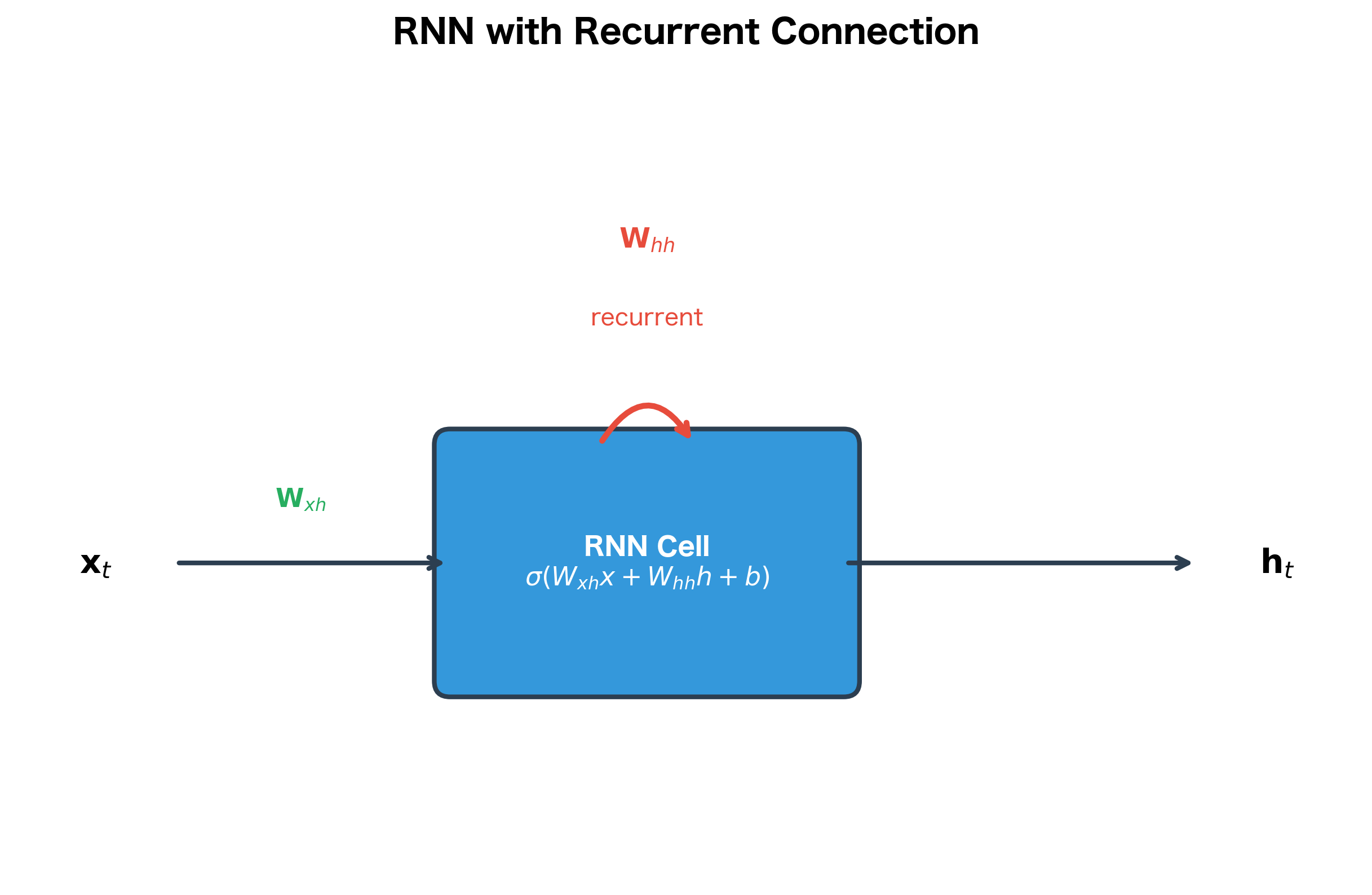
The self-loop in the diagram represents the recurrent connection. At each time step, the hidden state is computed using both the current input and the previous hidden state . This creates a chain of dependencies that allows information to flow through time.
Hidden State as Memory
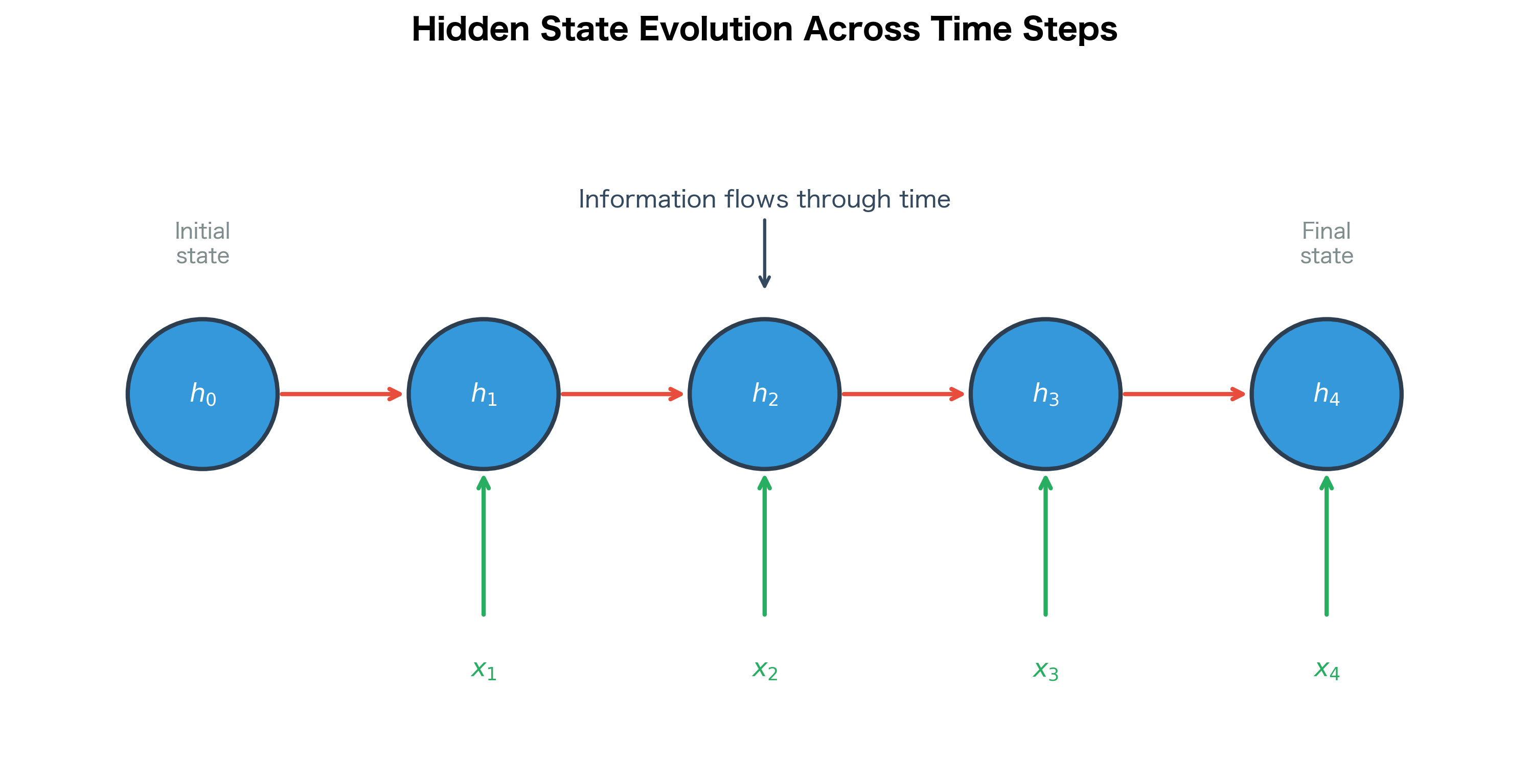
The hidden state is the RNN's memory. It's a fixed-size vector that encodes a summary of all the inputs the network has seen up to time . Think of it as a compressed representation of the sequence history.
At time step 0, before the RNN has seen any inputs, we typically initialize the hidden state to a zero vector:
where is a vector of zeros with the same dimension as the hidden state.
As the RNN processes each input, the hidden state evolves to incorporate new information:
- encodes information about
- encodes information about and
- encodes information about
The hidden state doesn't store the raw inputs. Instead, it learns to extract and compress the features that are relevant for the task. For language modeling, this might include syntactic structure, semantic meaning, and discourse context. For time series prediction, it might capture trends, seasonality, and recent fluctuations.
The key insight is that the hidden state size is fixed regardless of sequence length. Whether processing a 5-word sentence or a 500-word document, the RNN compresses all relevant information into a vector of the same dimension. This is both a strength (constant memory usage) and a limitation (finite capacity to store long-range dependencies).
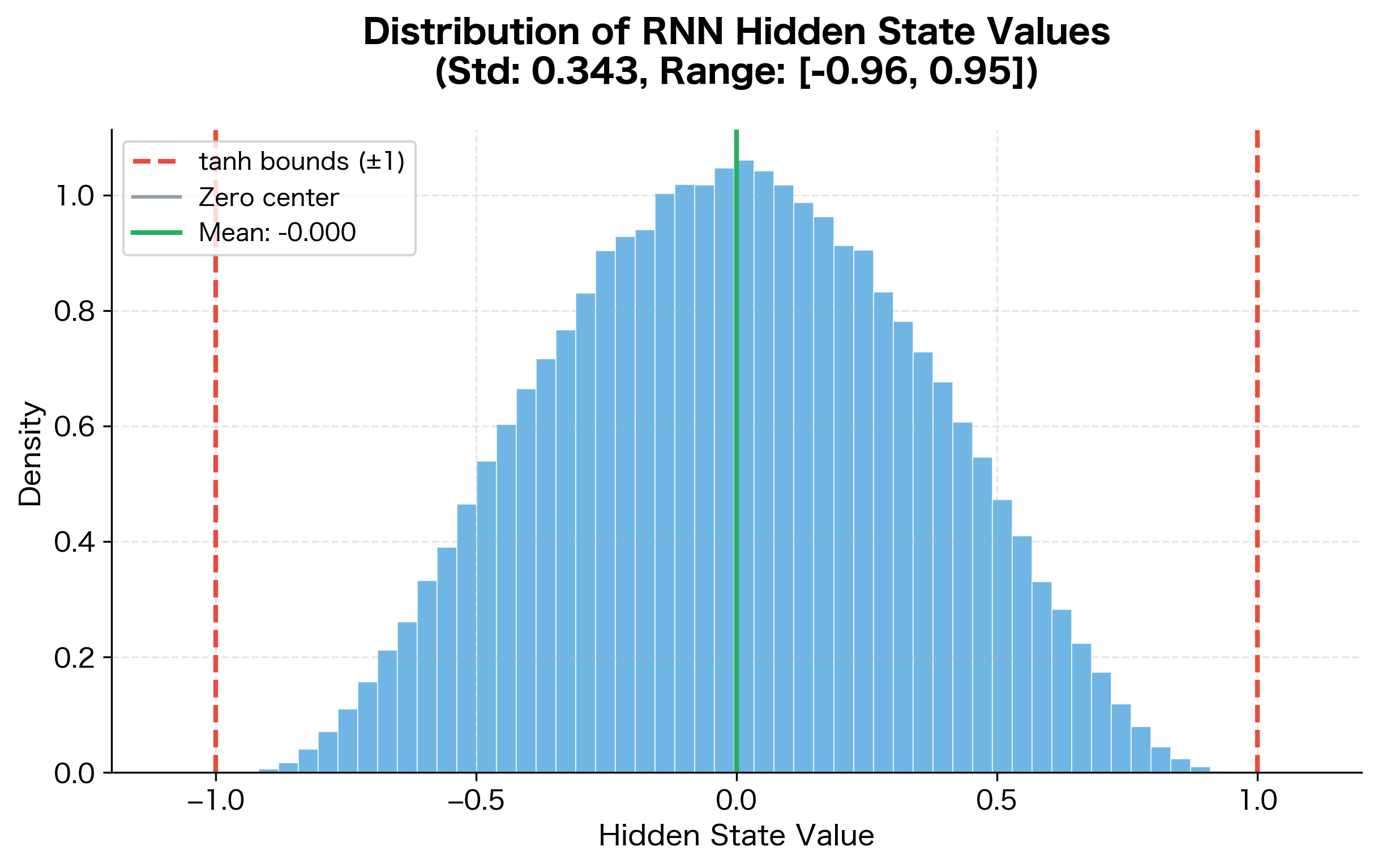
This distribution reveals that the activation keeps hidden state values well-behaved. Most values cluster near zero, with the distribution tapering off toward the bounds at . This zero-centered property is important for gradient flow during training.
Unrolling the Computation Graph
To understand how gradients flow through an RNN during training, we "unroll" the recurrent loop across time. This transforms the compact diagram with a self-loop into an explicit computational graph where each time step is a separate node.
The unrolled view reveals that an RNN is essentially a very deep feedforward network, with one layer per time step. The crucial difference is that the same weights are shared across all time steps.
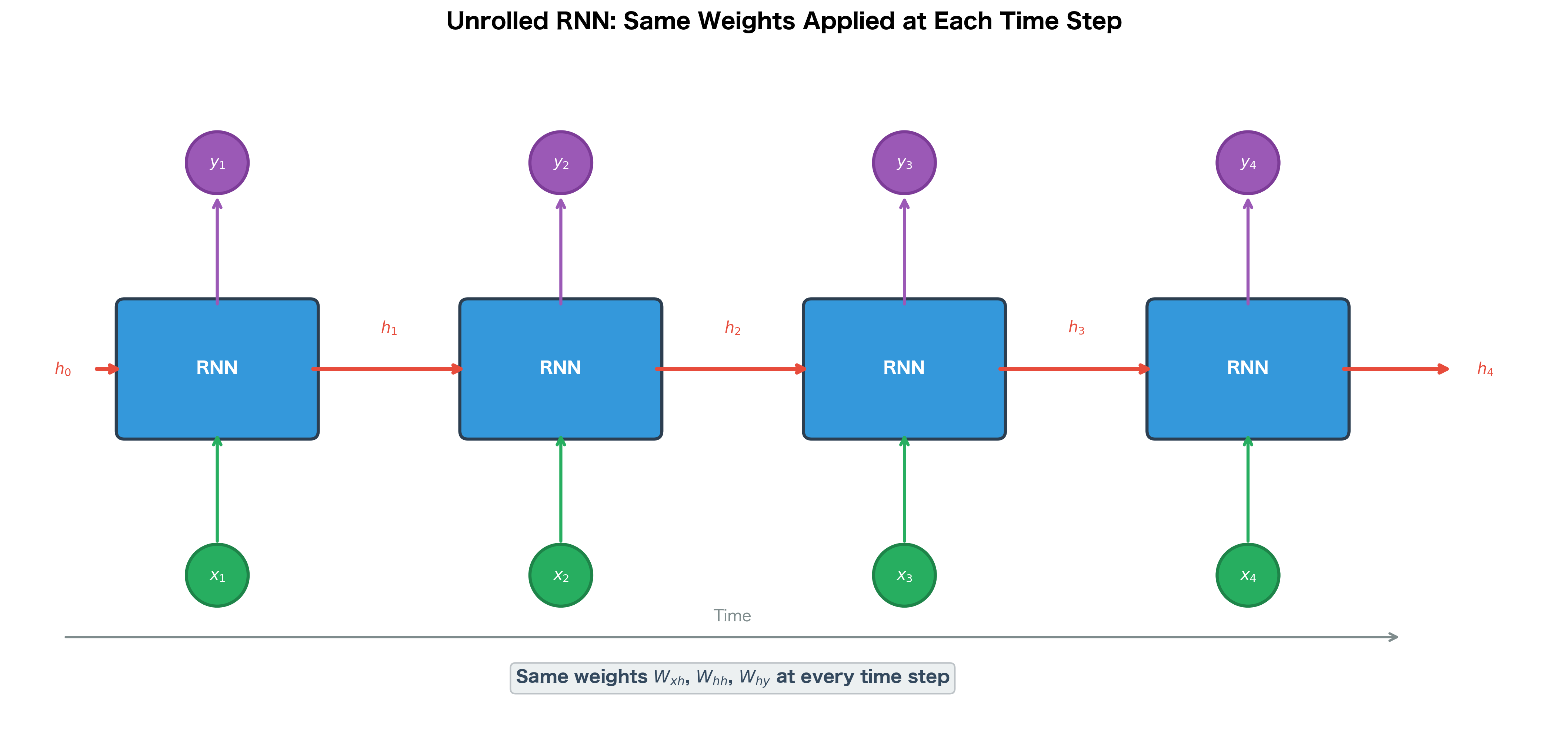
The unrolled graph makes several things clear:
- Depth: An RNN processing a sequence of length is effectively a -layer deep network, where is the number of time steps. This depth is what makes training RNNs challenging, as we'll see in later chapters on vanishing gradients.
- Weight sharing: The same , , and matrices appear at every time step. This dramatically reduces the number of parameters compared to having separate weights for each position.
- Gradient flow: During backpropagation, gradients must flow backward through all time steps. This is called Backpropagation Through Time (BPTT), which we'll cover in the next chapter.
Parameter Sharing Across Time
Parameter sharing is a fundamental design choice in RNNs. The same weights are used to process the input at every time step, regardless of position in the sequence.
This has several important implications:
Generalization to variable lengths: Because the weights don't depend on position, an RNN trained on sequences of length 10 can process sequences of length 100 or 1000 without any modification. The network learns transformations that apply universally across time steps.
Statistical strength: If a pattern (like "not" negating sentiment) can appear anywhere in a sequence, parameter sharing means the network learns this pattern once and applies it everywhere. Without sharing, the network would need to learn the same pattern separately for each position.
Reduced parameters: A feedforward network processing a sequence of length with hidden size would need parameters if each position had separate weights. An RNN needs only parameters, independent of sequence length. Here, represents the number of time steps and is the hidden state dimension.
The RNN has just over 6,000 parameters, regardless of sequence length. The parameter count is independent of sequence length. Whether we process 10 tokens or 10,000 tokens, the RNN uses exactly the same 6,208 parameters. This efficiency is crucial for processing long sequences like documents or time series.
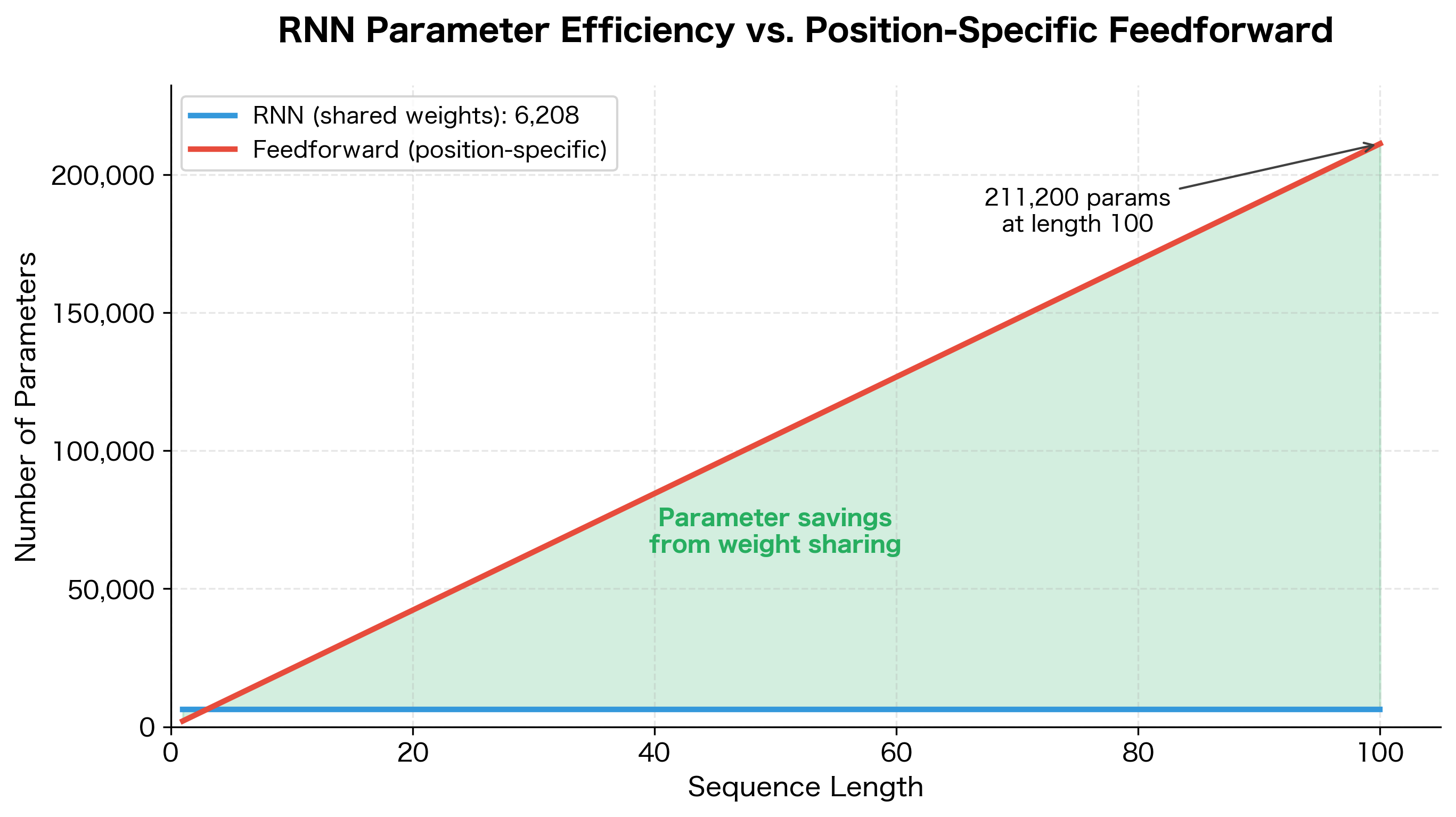
This visualization makes the efficiency of parameter sharing concrete. The RNN's flat line represents constant memory footprint regardless of sequence length, while the feedforward approach's linear growth quickly becomes impractical for long sequences.
The RNN Equations
Now that we understand the intuition behind recurrent connections and hidden states, let's formalize the mathematics that make RNNs work. The goal is to derive equations that capture two essential operations: updating the network's memory based on new input, and producing outputs based on that memory.
The Core Challenge: Combining Past and Present
At each time step, an RNN faces a fundamental question: how should it blend information from the current input with what it already knows from the past? This isn't trivial. The network needs to:
- Extract relevant features from the current input
- Retain useful information from the previous hidden state
- Combine these sources in a way that produces a useful new representation
The elegant solution is to use separate learned transformations for each information source, then add them together before applying a nonlinearity.
The Hidden State Update Equation
The hidden state update is the heart of the RNN. It determines how the network's memory evolves as it processes each new input:
Let's unpack this equation piece by piece to understand why each component is necessary.
The input transformation projects the current input into the hidden space. The weight matrix learns which aspects of the input are relevant for the task. For example, in language modeling, it might learn to emphasize semantic features of word embeddings while downweighting noise.
The recurrent transformation determines how past information influences the present. This is the "memory" mechanism. The matrix learns which aspects of the previous hidden state should persist and how they should be transformed. Some dimensions might carry long-term information (like sentence topic), while others track short-term patterns (like recent words).
The bias term provides a learnable offset, allowing the network to shift its activation patterns. This is particularly useful for controlling the default behavior when inputs are near zero.
The addition of these three terms is crucial. By summing the contributions, the network can learn to weight past and present information appropriately. If has small values, the network emphasizes current input. If is small, it relies more on memory.
The activation serves two purposes. First, it introduces nonlinearity, allowing the network to learn complex patterns. Without it, stacking multiple time steps would collapse to a single linear transformation. Second, it bounds the output to , preventing the hidden state from growing without limit as the sequence progresses.
The Output Equation
Once we have the updated hidden state, we need to produce an output. This is typically a simple linear transformation:
The output layer maps from the hidden representation to the task-specific output space. For language modeling, might be logits over the vocabulary. For sentiment analysis, it might be scores for positive and negative classes.
Complete Variable Reference
To implement these equations correctly, you need to understand the shape and role of each variable:
- : input vector at time (e.g., a word embedding of dimension )
- : hidden state at time , the network's memory
- : hidden state from the previous time step
- : output at time (e.g., logits over a vocabulary of size )
- : input-to-hidden weight matrix, transforms -dimensional inputs to -dimensional hidden space
- : hidden-to-hidden (recurrent) weight matrix, determines how past information influences the present
- : hidden-to-output weight matrix, maps hidden state to output space
- : hidden bias vector
- : output bias vector
The activation squashes values to , centering the hidden state around zero. This zero-centered property helps with gradient flow compared to sigmoid (which outputs only positive values). However, still suffers from vanishing gradients for large inputs, a problem we'll address with LSTM and GRU architectures.
Dimension Analysis
Understanding the dimensions at each step is crucial for implementing RNNs correctly. Let's trace through a concrete example:
Implementing an RNN from Scratch
With the mathematical foundations in place, let's translate the equations into working code. We'll build the implementation incrementally, starting with the simplest possible unit (a single time step) and progressively adding complexity until we have a complete, reusable RNN.
This bottom-up approach serves two purposes: it reinforces the mathematical concepts by showing exactly how each equation maps to code, and it produces modular components that are easy to test and debug.
Single Time Step
The atomic unit of an RNN is the hidden state update for a single time step. This function directly implements the equation :
The output shape confirms that our rnn_step function correctly transforms inputs of shape (batch_size, input_dim) to hidden states of shape (batch_size, hidden_dim). The hidden state values fall within the expected range due to the activation.
Full Sequence Processing
A single time step is useful, but real applications require processing entire sequences. The key insight is that we simply loop through time, feeding each step's output hidden state as the next step's input. We also collect all hidden states, which proves useful for tasks like attention mechanisms or when we need outputs at every position:
The output shows that our RNN processes a batch of 4 sequences, each with 10 time steps and 8 input features, producing hidden states of dimension 16. The hidden state evolution demonstrates how values change at each time step as the network incorporates new information. Notice that the values remain bounded within due to the activation, and different dimensions evolve differently based on the learned weights.
Complete RNN Class
For practical use, we want to encapsulate the RNN's parameters and operations into a single object. The class below combines weight initialization, the forward pass, and utility methods. Notice how the forward pass now includes the output computation , making this a complete sequence-to-sequence model:
The SimpleRNN class encapsulates the full RNN computation. With an architecture of 64 input dimensions, 128 hidden units, and 100 output classes, the model has approximately 30,000 parameters. The forward pass processes all 15 time steps and returns outputs at each position, all hidden states for potential use in attention mechanisms, and the final hidden state for classification tasks.
RNN for Sequence Classification
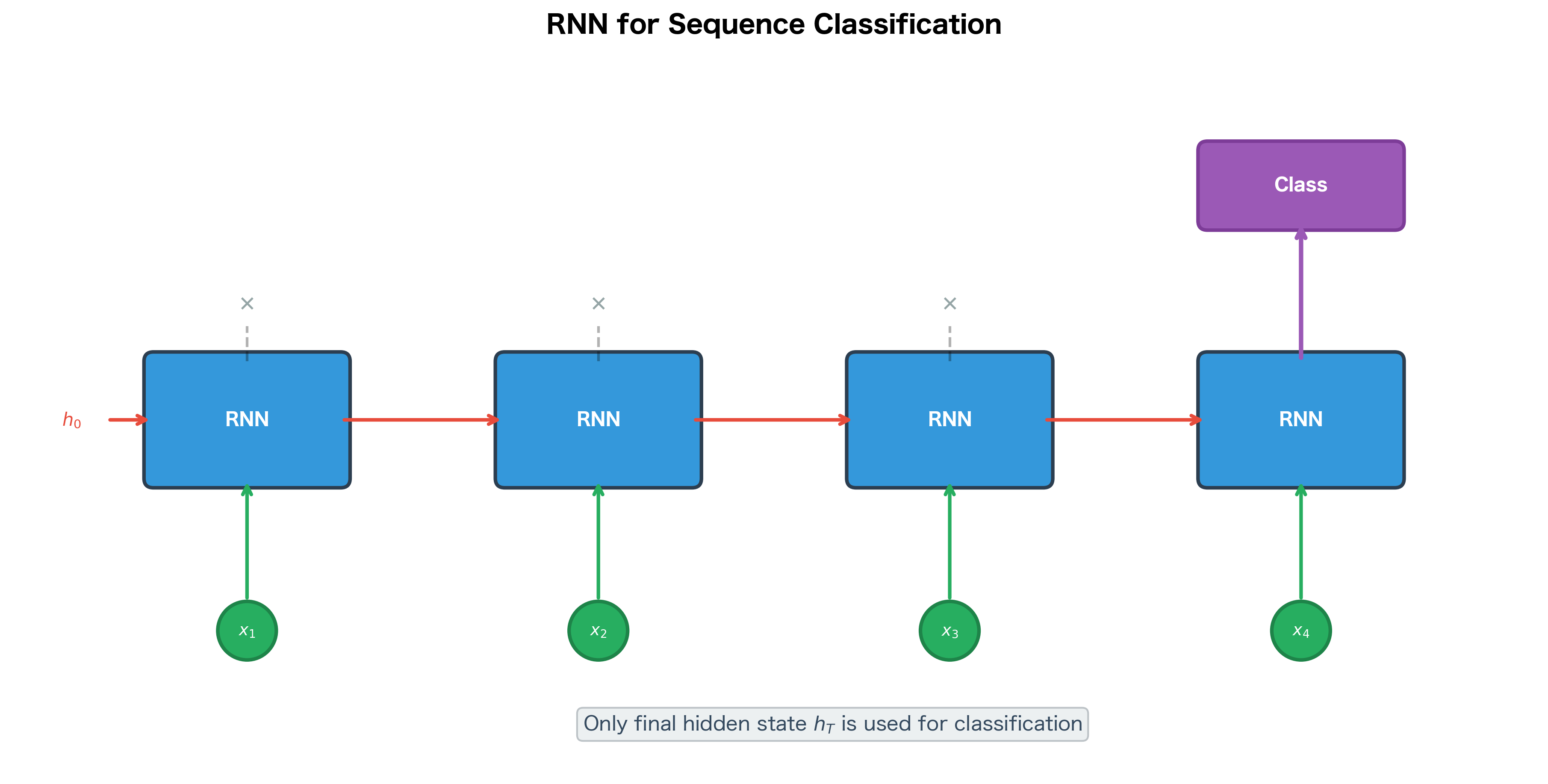
One common application of RNNs is sequence classification, where we want to assign a single label to an entire sequence. Examples include sentiment analysis (positive/negative), spam detection, and topic classification.
For sequence classification, we typically use only the final hidden state to make the prediction, where is the sequence length. This final state has "seen" the entire sequence and should encode all the information needed for classification.
The classification output shows logits for each sequence in the batch. After applying softmax to convert logits to probabilities, we see predictions for each sequence. With randomly initialized weights, the predictions are essentially random. After training on labeled sentiment data, the model would learn to produce high positive probabilities for positive reviews and high negative probabilities for negative reviews.
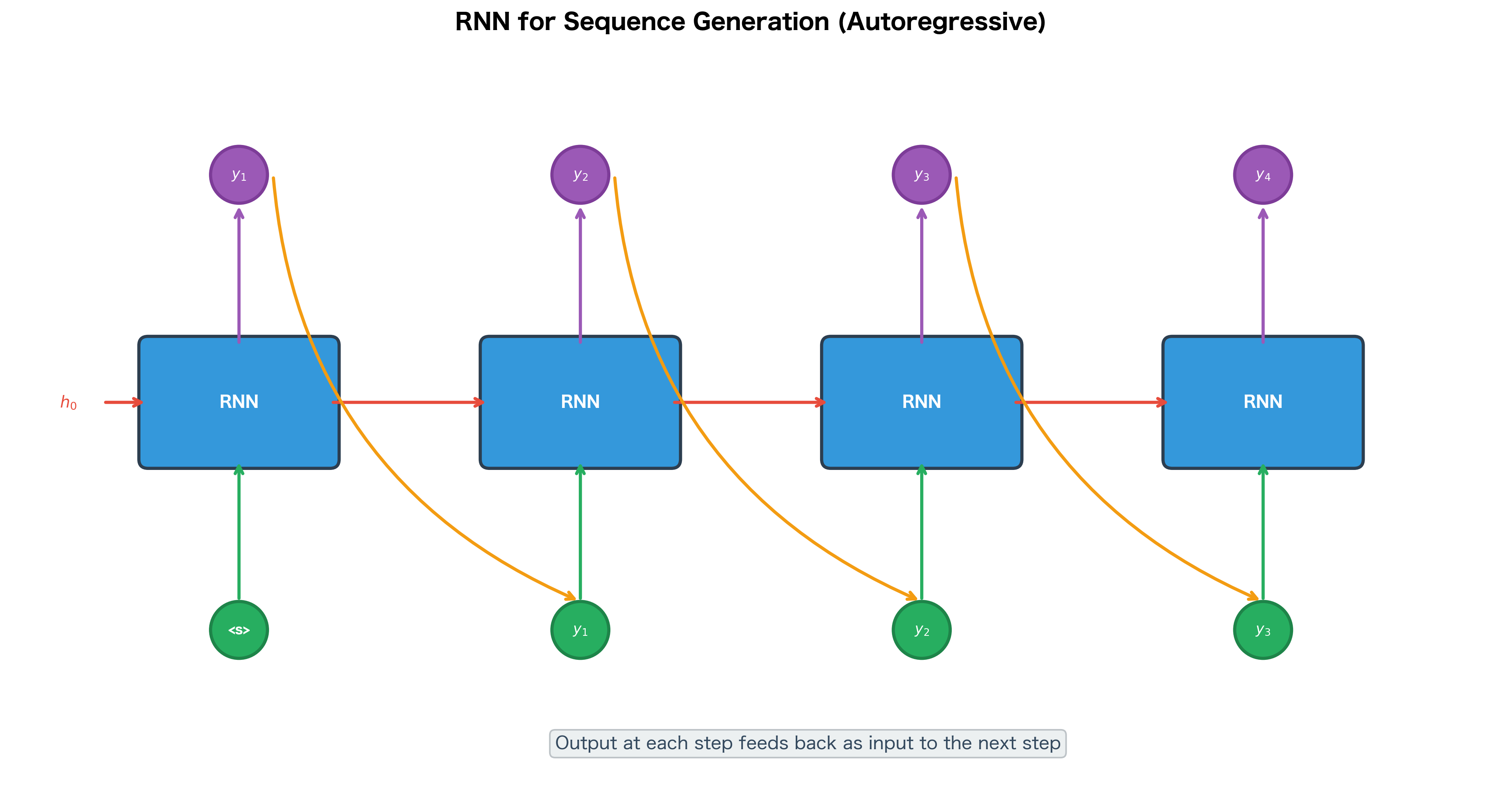
RNN for Sequence Generation
Another powerful application is sequence generation, where the RNN produces an output at each time step. This is used for language modeling, machine translation, and text generation.
In generation mode, the RNN's output at time becomes (part of) the input at time . This creates an autoregressive loop where the model generates one token at a time, conditioning on all previously generated tokens.
The generated sequence is a list of token indices sampled from the model's output distribution. With untrained, random weights, these indices have no semantic meaning. However, after training on a text corpus, the same generation procedure would produce coherent sequences. The temperature parameter controls randomness: lower values (e.g., 0.5) make the model more confident and deterministic, while higher values (e.g., 1.5) increase diversity but may reduce coherence.
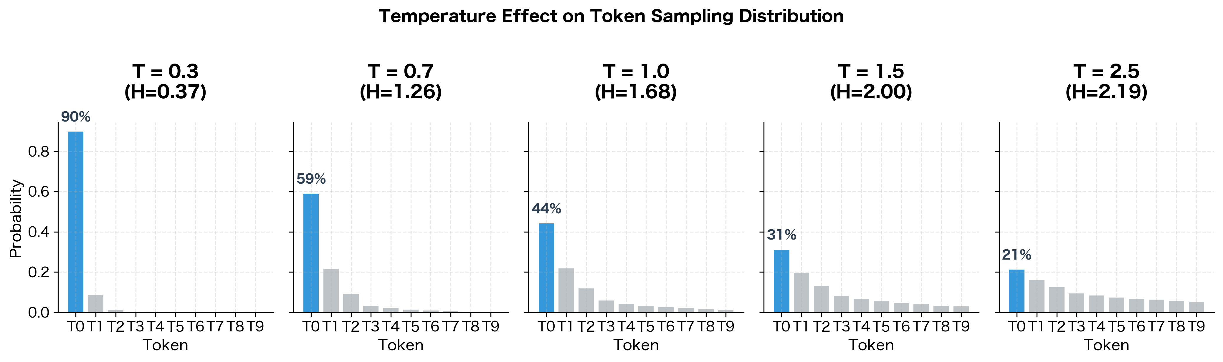
The entropy values (H) quantify the randomness of each distribution. At temperature 0.3, the model is nearly deterministic with 75% probability on the top token. At temperature 2.5, the distribution is much flatter, giving even unlikely tokens a reasonable chance of being sampled. Choosing the right temperature is a key decision when deploying generative models.
Visualizing Hidden State Dynamics
To build intuition about how RNNs process sequences, let's visualize how the hidden state evolves over time for different input patterns.
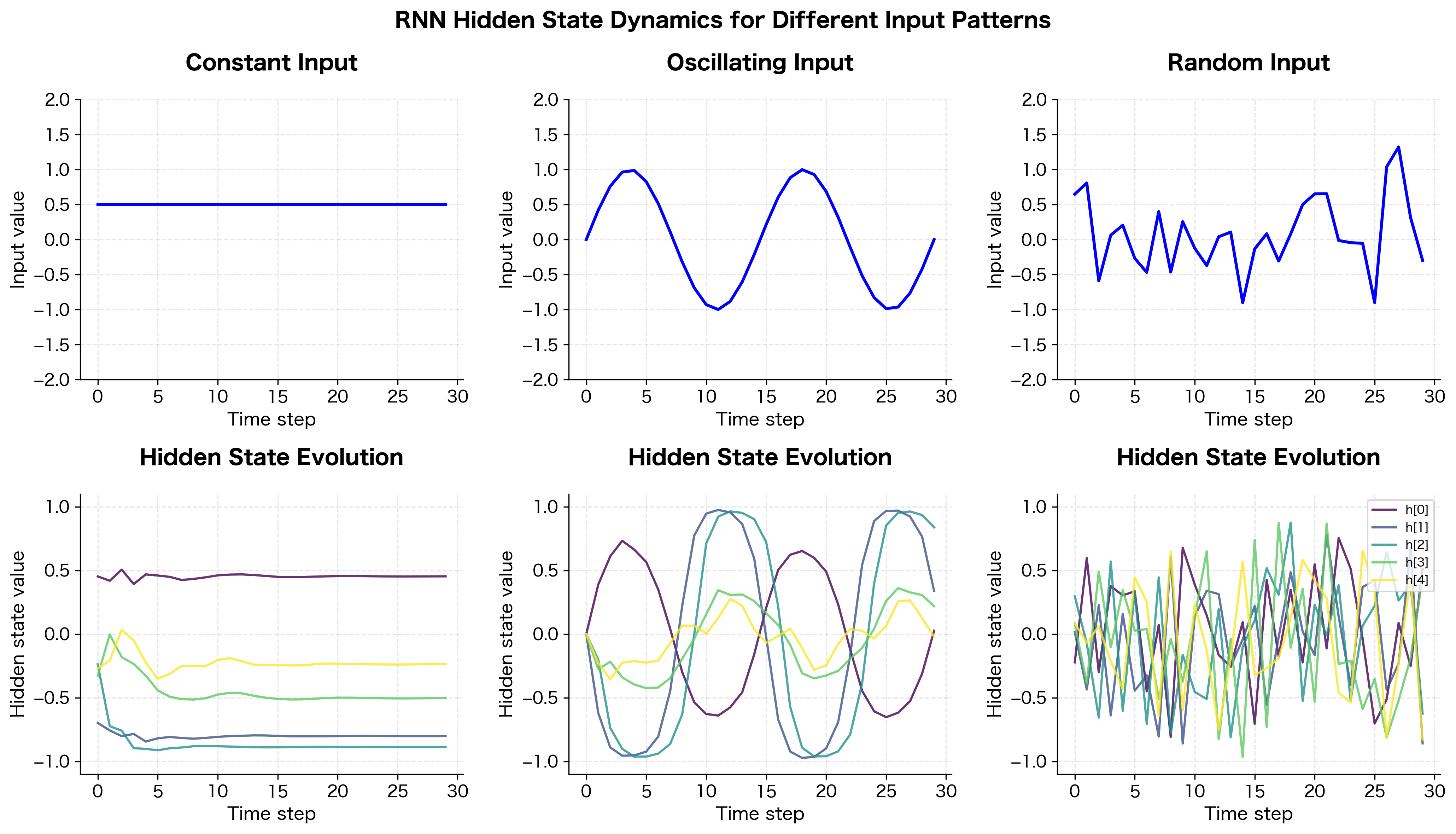
The visualization reveals several important properties of RNN dynamics:
- Constant input: The hidden state quickly converges to a fixed point. Once the network has "absorbed" the constant signal, the hidden state stops changing.
- Oscillating input: The hidden state tracks the oscillations, with different dimensions responding at different phases and amplitudes.
- Random input: The hidden state shows complex, chaotic dynamics as it tries to encode the unpredictable input stream.
These dynamics are determined by the recurrent weights . The eigenvalues of this matrix, which characterize how the matrix scales vectors in different directions, control whether the hidden state explodes, vanishes, or maintains stable dynamics over time. This is a topic we'll explore in depth in the chapter on vanishing gradients.
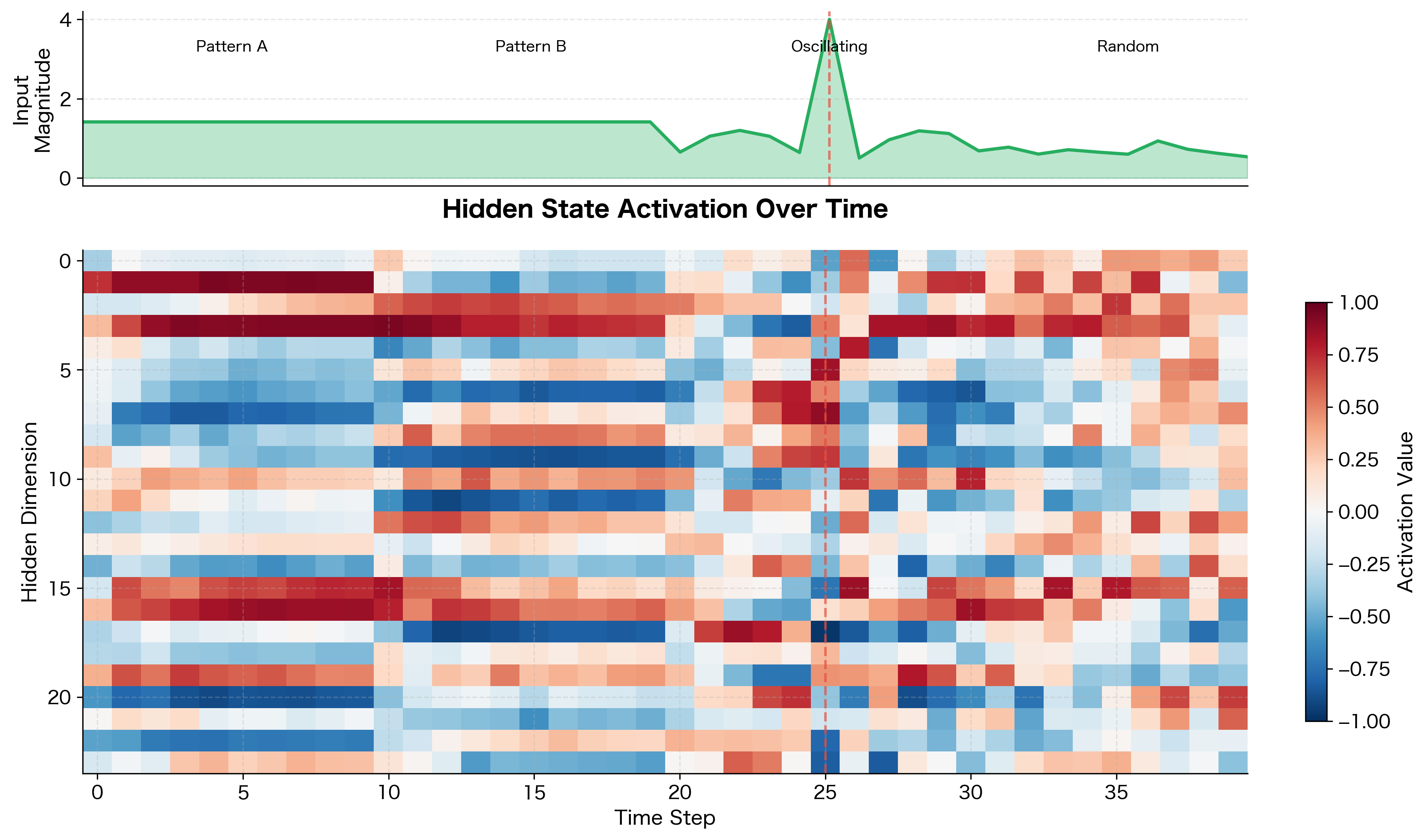
The heatmap reveals how different hidden dimensions specialize in tracking different aspects of the input. Some dimensions (horizontal bands of consistent color) act as "memory cells" that maintain their state over time. Others show rapid fluctuations in response to input changes. The spike at time step 25 creates a visible perturbation across many dimensions, demonstrating how the hidden state responds to sudden input changes.
Limitations and Impact
RNNs represented a major breakthrough in sequence modeling, but they come with significant limitations that motivated the development of more advanced architectures.
The Vanishing Gradient Problem
The most critical limitation of vanilla RNNs is the vanishing gradient problem. When training on long sequences, gradients must flow backward through many time steps. At each step, the gradient is multiplied by the recurrent weight matrix . If the largest eigenvalue of is less than 1, these repeated multiplications cause the gradient to shrink exponentially, effectively preventing the network from learning long-range dependencies.
Consider a sequence where a word at position 5 is crucial for predicting the word at position 50. The gradient signal from position 50 must traverse 45 time steps to influence the weights that process position 5. With vanishing gradients, this signal becomes negligibly small, and the network fails to learn the dependency. This is why vanilla RNNs struggle with tasks requiring memory over more than 10-20 time steps.
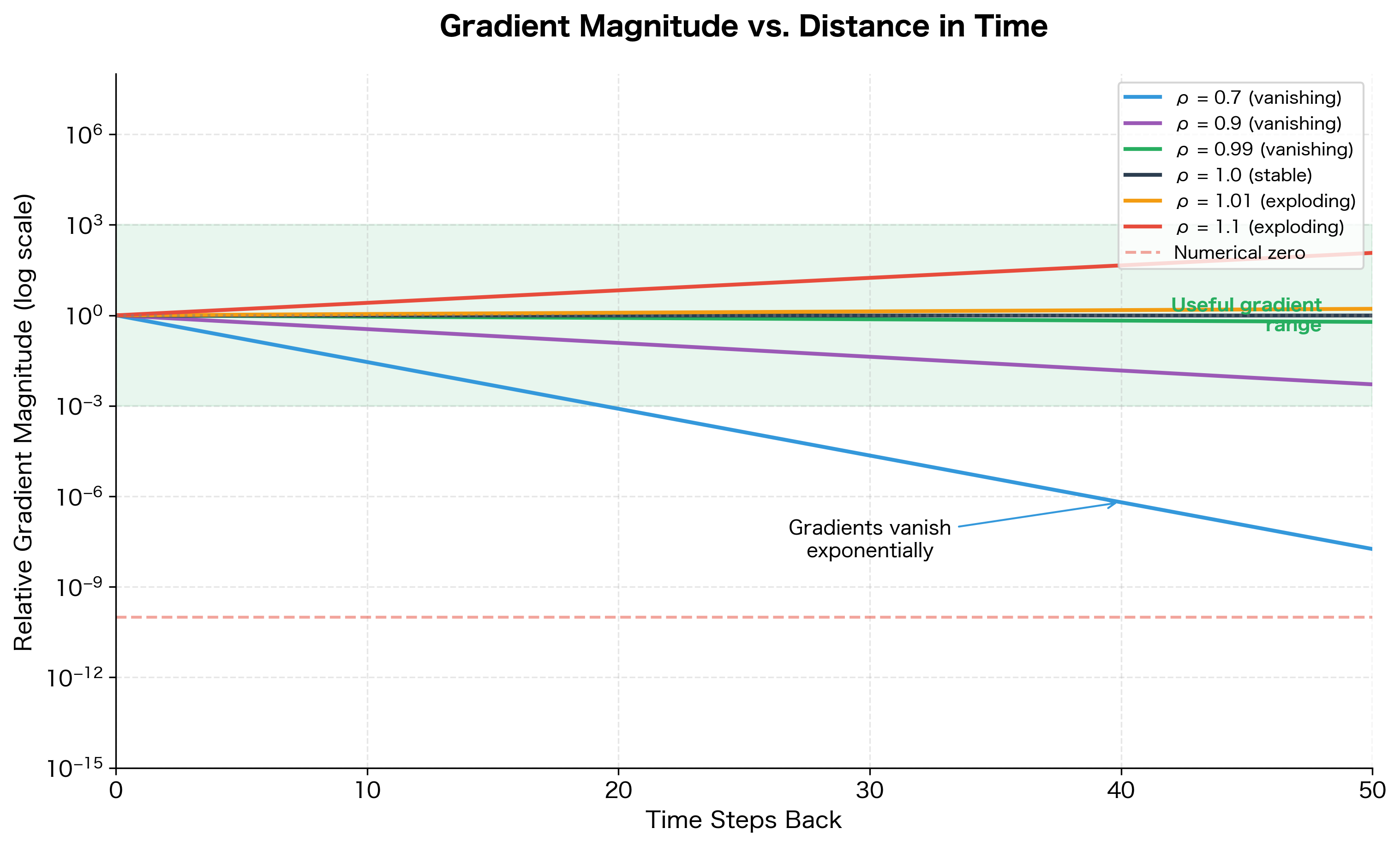
This visualization shows why vanilla RNNs struggle with long sequences. With a spectral radius of 0.9, the gradient is reduced to about 1% of its original magnitude after just 45 time steps. With 0.7, it becomes numerically zero after about 30 steps. The narrow band near where gradients remain useful is difficult to maintain during training, motivating the gated architectures (LSTM, GRU) that explicitly address this problem.
Sequential Computation Bottleneck
RNNs process sequences one step at a time, with each step depending on the previous one. This sequential dependency prevents parallelization during training. While a feedforward network can process all positions simultaneously, an RNN must wait for before computing . On modern GPUs designed for parallel computation, this sequential bottleneck significantly slows training on long sequences.
Historical Impact
Despite these limitations, RNNs were transformative for NLP and sequence modeling:
- Language modeling: RNNs enabled the first neural language models that could generate coherent text, moving beyond n-gram models.
- Machine translation: Sequence-to-sequence RNNs with attention (which we'll cover later) achieved state-of-the-art translation quality before transformers.
- Speech recognition: RNNs powered major advances in speech-to-text systems.
- Time series: RNNs remain useful for many time series forecasting applications where sequences are short enough to avoid gradient issues.
The limitations of vanilla RNNs directly motivated the development of LSTM and GRU architectures, which use gating mechanisms to create "gradient highways" that allow information to flow over long distances. These architectures dominated NLP from roughly 2014-2017, until transformers provided an even more effective solution to the long-range dependency problem.
Summary
This chapter introduced the fundamental architecture of Recurrent Neural Networks:
-
Recurrent connections create memory by feeding the hidden state back into itself, allowing RNNs to process sequential data with temporal dependencies.
-
Hidden state acts as a compressed summary of all previous inputs, evolving at each time step through the equation .
-
Parameter sharing across time steps means the same weights process every position, enabling RNNs to handle variable-length sequences with a fixed number of parameters.
-
Unrolling the computation graph reveals that an RNN is effectively a deep network with one layer per time step, which is crucial for understanding gradient flow during training.
-
Sequence classification uses the final hidden state to make predictions about entire sequences, while sequence generation produces outputs at each step in an autoregressive loop.
-
Limitations include vanishing gradients that prevent learning long-range dependencies and sequential computation that prevents parallelization.
In the next chapter, we'll examine how to train RNNs using Backpropagation Through Time (BPTT), understanding exactly how gradients flow backward through the unrolled computation graph.
Key Parameters
When implementing RNNs, several hyperparameters significantly impact model performance:
-
hidden_dim: The dimension of the hidden state vector. Larger values increase the model's capacity to store information but also increase computation and risk of overfitting. Typical values range from 64 to 512 for most NLP tasks.
-
input_dim: The dimension of input vectors, often determined by the embedding size. Common choices are 100, 200, or 300 for word embeddings.
-
num_layers: The number of stacked RNN layers. Deeper networks can learn more complex patterns but are harder to train. Most applications use 1-3 layers.
-
activation: The activation function applied to the hidden state. The default works well for most cases, keeping values bounded in .
-
initial_hidden_state: How to initialize . Zero initialization is standard, though learned initial states can sometimes improve performance.
-
temperature (for generation): Controls the randomness of sampling during sequence generation. Values below 1.0 make outputs more deterministic; values above 1.0 increase diversity.
Quiz
Ready to test your understanding? Take this quick quiz to reinforce what you've learned about RNN architecture.

Comments