

Master neural network loss functions from MSE to cross-entropy, including numerical stability, label smoothing, and focal loss for imbalanced data.

This article is part of the free-to-read Language AI Handbook
Choose your expertise level to adjust how many terms are explained. Beginners see more tooltips, experts see fewer to maintain reading flow. Hover over underlined terms for instant definitions.
Loss Functions
How does a neural network know it's wrong? When a model predicts that a movie review is positive but it's actually negative, something needs to measure that mistake. Loss functions quantify the difference between predictions and ground truth, providing the signal that guides learning. Without a loss function, a neural network has no compass, no way to improve.
In the previous chapters, we built the forward pass: data flows through layers, activations introduce non-linearity, and the network produces an output. But that output needs to be evaluated. Loss functions sit at the end of the forward pass, taking predictions and true labels, and producing a single number that summarizes how wrong the model is. This number then flows backward through backpropagation, telling each parameter how to adjust.
This chapter explores the mathematical foundations of loss functions, starting with mean squared error for regression and cross-entropy for classification. You'll learn why cross-entropy works better than squared error for classification, how to handle numerical stability issues that plague naive implementations, and advanced techniques like label smoothing and focal loss that address real-world challenges. By the end, you'll understand how to choose, implement, and even design custom loss functions for your specific needs.
The Role of Loss Functions
Before diving into specific formulas, let's establish what loss functions do and why they matter so much. A loss function serves three interconnected purposes.
First, it provides an optimization objective. Neural networks learn by minimizing a loss function through gradient descent. The loss surface defines the landscape the optimizer navigates, and the choice of loss function shapes that landscape. Smooth loss surfaces with clear gradients lead to stable training, while poorly chosen losses can create plateaus, sharp cliffs, or misleading local minima.
Second, it encodes the task. Different problems require different notions of "correctness." Predicting house prices within $10,000 is very different from predicting whether an email is spam. The loss function translates task requirements into mathematical objectives. Regression losses measure distance from target values, while classification losses measure how confidently the model assigns probability to the correct class.
Third, it shapes the gradients. During backpropagation, the gradient of the loss with respect to predictions determines how strongly each parameter gets updated. Some loss functions produce gradients that are proportional to the error magnitude, while others produce gradients that depend on confidence levels. This distinction profoundly affects training dynamics.
A loss function (also called cost function or objective function) maps model predictions and ground truth labels to a non-negative scalar that quantifies prediction error:
where:
- : the model's predictions (a vector of values)
- : the ground truth labels
- : the loss value, typically non-negative, where 0 indicates perfect prediction
The goal of training is to find parameters that minimize the expected loss over the training data.
Mean Squared Error for Regression
We start with the most intuitive loss function: mean squared error (MSE). When predicting continuous values, like house prices, stock returns, or temperature, we want predictions close to targets. MSE measures the average squared distance between predictions and targets.
Mathematical Formulation
For a single prediction, the squared error is simply the squared difference between prediction and target:
where:
- : the model's prediction for this sample
- : the true target value
- : the squared error, always non-negative
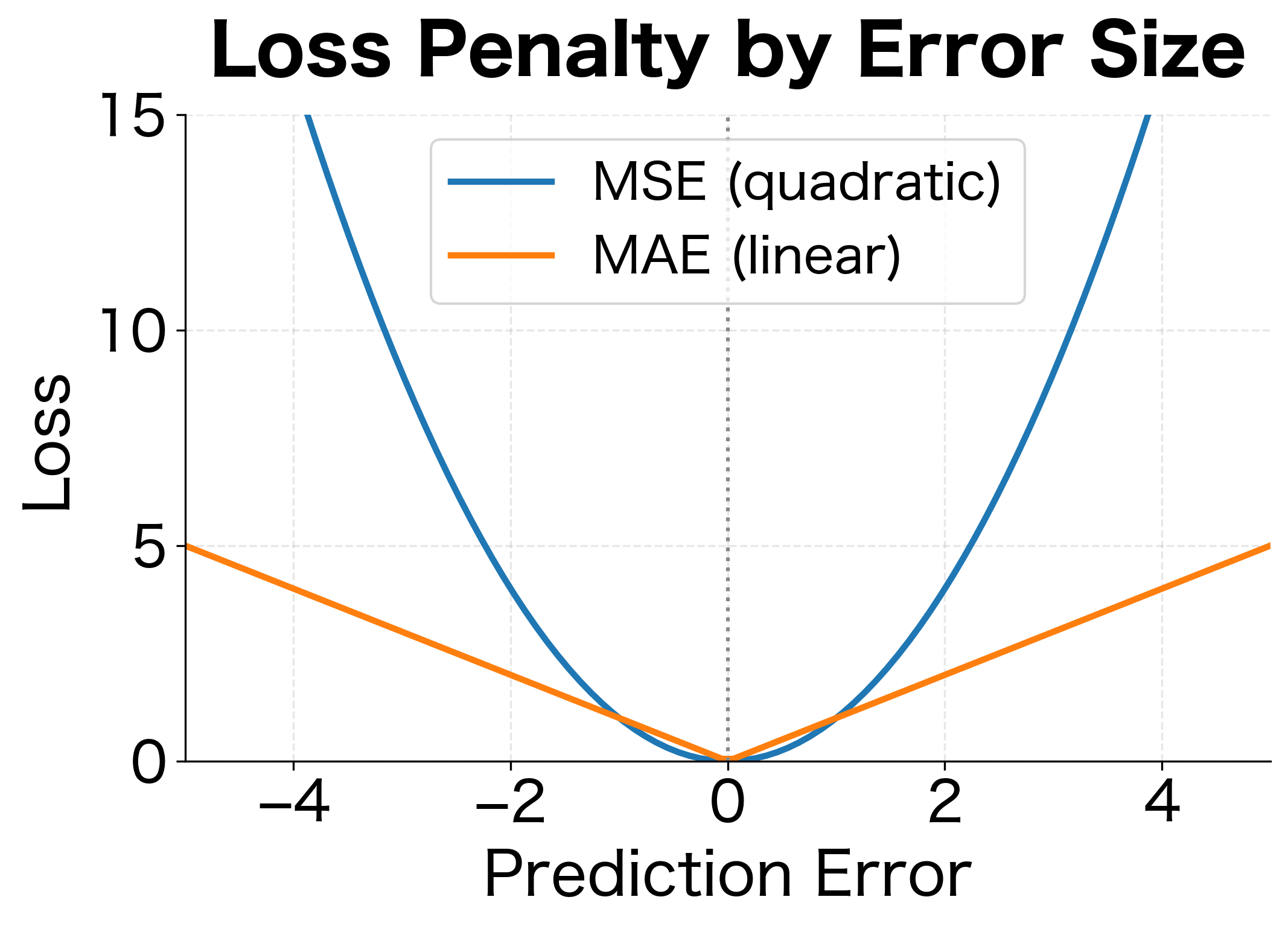
Squaring serves two purposes. It makes all errors positive (a prediction 5 units too high is as bad as 5 units too low), and it penalizes large errors more heavily than small ones. An error of 10 contributes 100 to the loss, while an error of 1 contributes only 1.
MSE averages the squared errors across all samples in a batch:
where:
- : the number of samples in the batch
- : the model's prediction for sample
- : the true target value for sample
- The factor normalizes the loss so it doesn't grow with batch size
Why Squared Error?
Why square the error rather than take its absolute value, cube it, or use some other function? The answer lies in a beautiful connection between MSE and probability theory that reveals the hidden assumptions behind this seemingly arbitrary choice.
Imagine you're predicting house prices. Even with a perfect model, your predictions won't be exactly right because of factors you can't observe: the seller's mood, minor undisclosed repairs, or market fluctuations on the day of sale. These unobserved factors create random noise around the true relationship. The central limit theorem tells us that when many small, independent factors combine, their sum tends toward a Gaussian (normal) distribution. This is why assuming Gaussian noise is often reasonable.
Under this assumption, the observed target equals the model's prediction plus some random noise :
where:
- : the observed target value
- : the model's prediction
- : the random noise term, drawn from a Gaussian distribution
- : the variance of the noise (how spread out the errors are)
- : the Gaussian (normal) distribution with mean 0 and variance
Now we can ask: given our prediction , what's the probability of observing the actual target ? The Gaussian distribution gives us this probability, and taking its logarithm (for computational convenience and to turn products into sums) yields:
where:
- : the log-probability of observing given that the model predicted
- : a negative scaling factor (since , this term is always negative)
- : the squared error between target and prediction
- : terms that don't depend on and thus don't affect optimization
The key insight is that maximizing this log-likelihood, which means finding predictions that make the observed data most probable, is mathematically equivalent to minimizing the squared error . The negative sign flips maximization to minimization, and the constant scaling factor doesn't change which prediction is optimal.
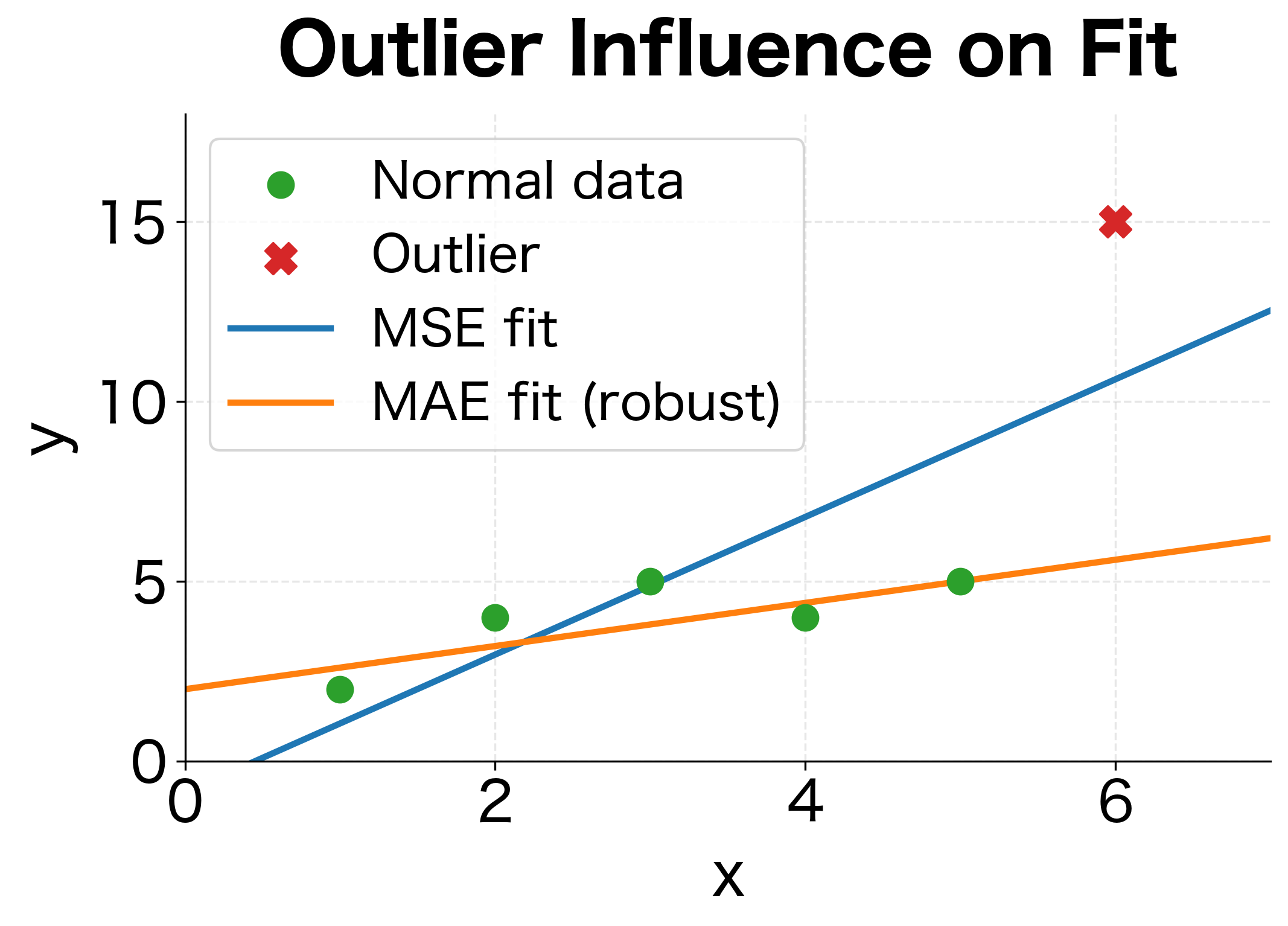
This probabilistic interpretation has profound implications. When you minimize MSE, you're implicitly assuming that prediction errors follow a Gaussian distribution. If errors actually follow a different distribution, like one with heavy tails where outliers are common, MSE may not be the best choice. This is why robust alternatives like Mean Absolute Error (MAE) exist for situations where outliers are prevalent.
Implementation
Let's implement MSE from scratch and verify against PyTorch's built-in implementation:
The values match, confirming our implementation is correct. The tiny difference (if any) comes from floating-point precision.
The MSE Gradient
Understanding the gradient of MSE reveals why it works well for regression. Taking the derivative with respect to a single prediction :
where:
- : the partial derivative of the loss with respect to prediction , telling us how to adjust to reduce loss
- : a scaling factor arising from the derivative of (which gives ) and the averaging
- : the prediction error, positive if prediction is too high, negative if too low
This gradient has an elegant property: it's proportional to the error itself. If a prediction is 10 units too high, the gradient pushes it down with magnitude proportional to 10. If a prediction is 0.1 units too high, the gradient is proportionally smaller. This linear relationship between error and gradient leads to stable, predictable learning dynamics.
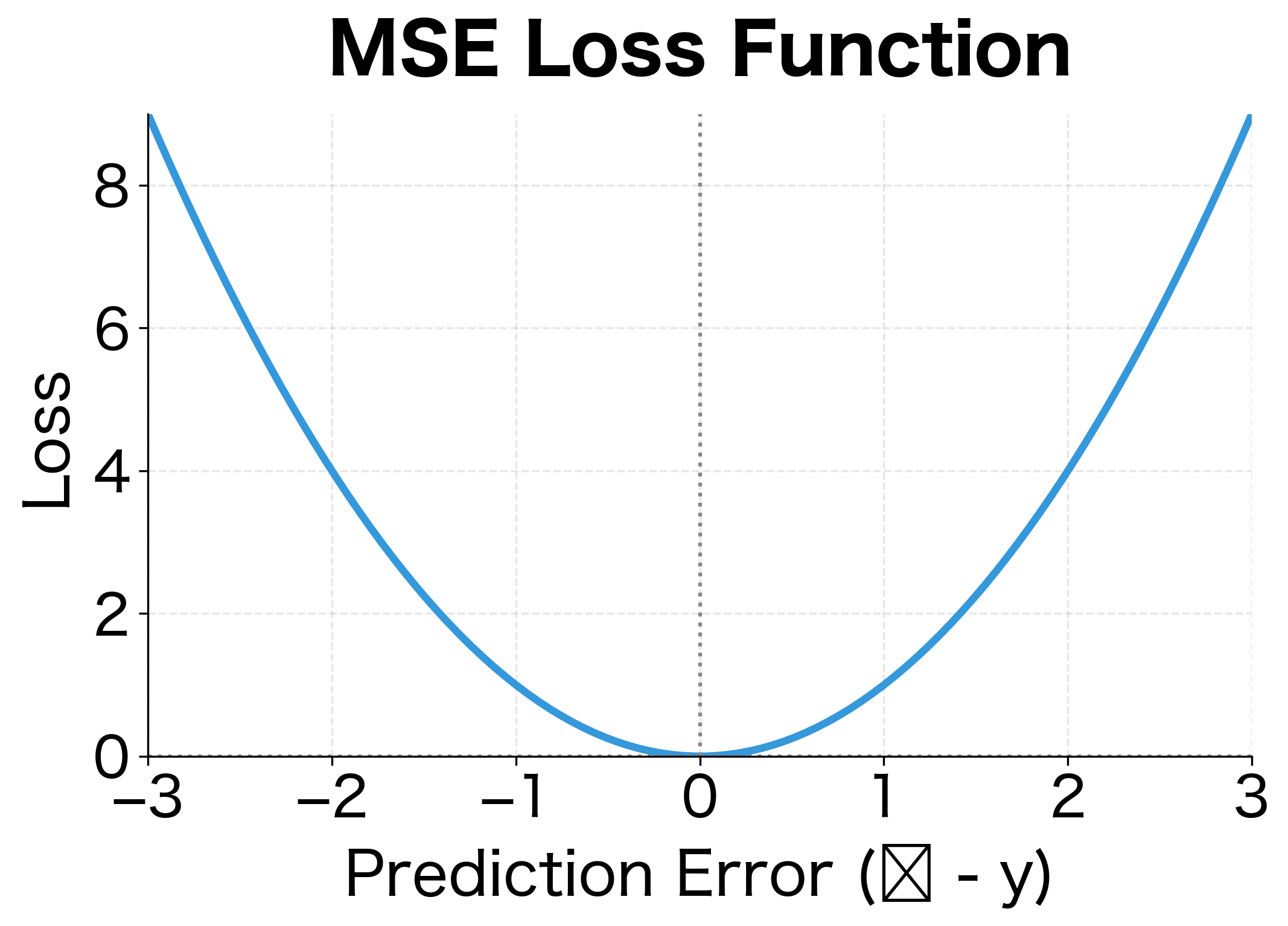
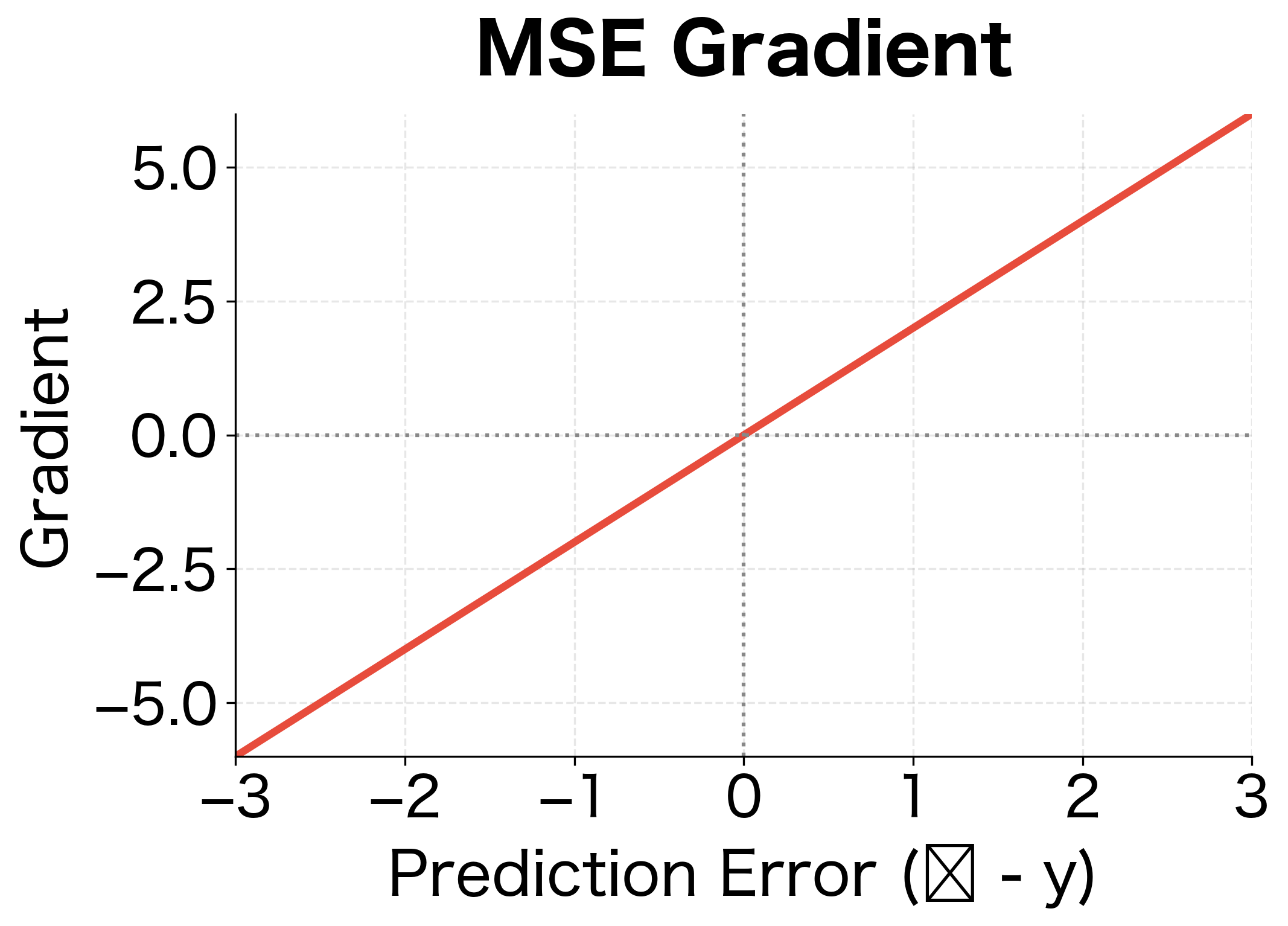
The parabolic loss curve and linear gradient are hallmarks of MSE. The minimum occurs exactly at zero error, and the gradient always points toward that minimum. However, the quadratic penalty means MSE is sensitive to outliers: a single prediction with error 10 contributes as much loss as 100 predictions with error 1.
Binary Cross-Entropy Loss
Regression predicts continuous values, but classification predicts discrete categories. For binary classification (two classes), we need a different approach. The model outputs a probability that the input belongs to class 1, and we need to measure how well that probability matches the true label .
Why Not Use MSE for Classification?
It's tempting to apply MSE to classification: just measure the squared difference between predicted probability and target label. Let's see why this fails.
Consider a sample with true label (positive class). The model predicts (90% confident it's positive). The MSE is , a small loss. Now suppose the model predicts (90% confident it's negative, wrong!). The MSE is , still less than 1.
The problem is the gradient. For MSE, . When and , the gradient is . But sigmoid outputs saturate at extreme values, producing near-zero gradients. The loss wants to push the probability higher, but the sigmoid's vanishing gradient prevents effective learning. This is the infamous vanishing gradient problem for classification.
Cross-entropy solves this by producing gradients that don't depend on the sigmoid's derivative.
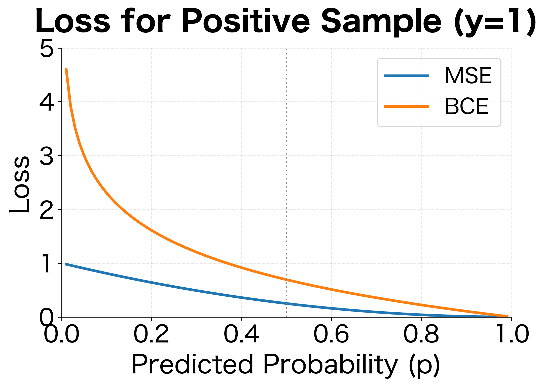
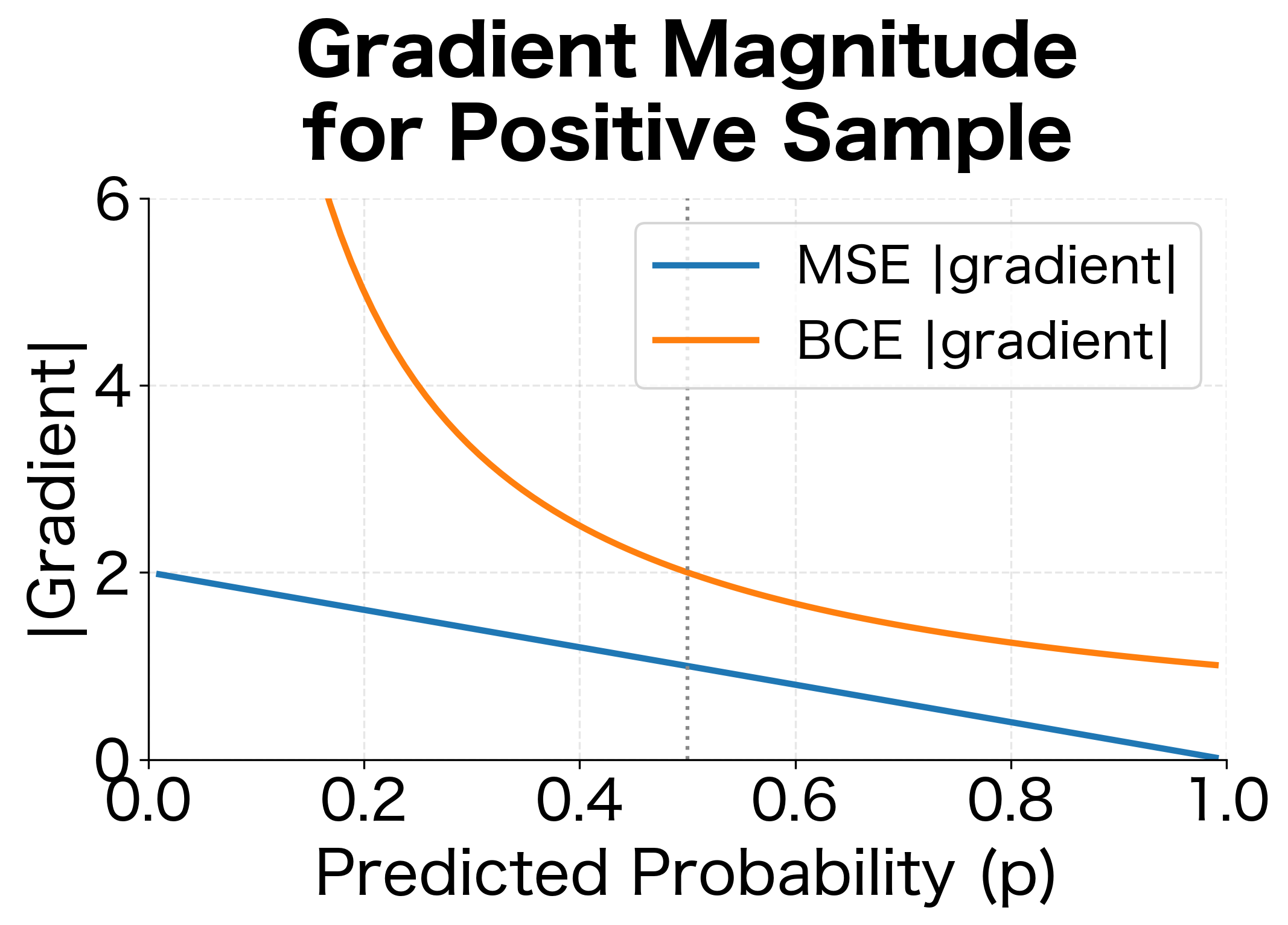
The visualization reveals the critical difference. When the model confidently predicts for a true positive (), MSE gives a loss of only 0.81 with a gradient magnitude of about 1.8. BCE gives a loss of 2.3 with a gradient magnitude of 10, over 5 times stronger. This stronger signal helps overcome the vanishing gradients from sigmoid saturation, making BCE far more effective for classification.
Mathematical Derivation
To derive binary cross-entropy, we need to think about classification from a probabilistic perspective. The model outputs a probability that a sample belongs to class 1. What we want is to find the that makes the observed label most likely. This is the principle of maximum likelihood estimation.
Consider what "likelihood" means here. If the true label is (positive class), then the model should output a high probability . The likelihood of observing given prediction is simply itself: a model predicting makes observing a positive label 90% likely. Conversely, if (negative class), the likelihood of observing this given prediction is : a model predicting makes observing a negative label 90% likely.
We can express both cases in a single elegant formula using exponents:
where:
- : the probability of observing label given the model's predicted probability
- : the model's predicted probability for class 1 (must be between 0 and 1)
- : the true label
- : equals when , equals when (since any number to the power of 0 is 1)
- : equals when , equals when
The beauty of this formula is how the exponents act as switches. When , the formula simplifies to . When , it becomes . One formula handles both cases.
Now, we want to maximize this likelihood, but maximization is less convenient than minimization for gradient descent. Also, products of probabilities (which arise when we have multiple samples) become sums when we take logarithms, which is numerically more stable. So we take the negative log:
where:
- : the negative log-likelihood, our loss function
- : the loss contribution when the true class is 1 (penalizes low )
- : the loss contribution when the true class is 0 (penalizes high )
This is the binary cross-entropy for a single sample. The logarithm has a crucial property: approaches infinity as approaches 0. This means confident wrong predictions (like when ) incur enormous penalties, while confident correct predictions (like when ) incur almost no penalty. The loss function naturally focuses learning on the mistakes that matter most.
Binary cross-entropy measures the negative log-likelihood for binary classification:
where:
- : number of samples
- : true label for sample
- : predicted probability of class 1 for sample
- : natural logarithm
The loss approaches 0 when predictions are confident and correct, and approaches infinity when predictions are confident and wrong.
Understanding the BCE Terms
The formula has two terms that activate depending on the true label:
- When : Only contributes. If , loss is near 0. If , loss explodes toward infinity.
- When : Only contributes. If , loss is near 0. If , loss explodes.
This asymmetry is exactly what we want. A confident wrong prediction (predicting when ) incurs a huge penalty, forcing the model to avoid overconfident mistakes.
Our implementation matches PyTorch's built-in BCE loss, confirming the correctness of our formula. The loss value of approximately 0.35 reflects a reasonably good model since predictions correlate with true labels, but not perfectly, as we intentionally added noise to simulate real-world imperfection.
The BCE Gradient
The gradient of BCE with respect to predicted probability reveals why it works so well:
where:
- : the derivative of the loss with respect to the predicted probability
- : the gradient contribution when , which is large (negative) when is small
- : the gradient contribution when , which is large (positive) when is close to 1
For a single sample with , this simplifies to:
When is small (wrong prediction), the gradient magnitude is large, producing strong corrective signal. When is close to 1 (correct prediction), the gradient is small, leaving good predictions relatively undisturbed.
Critically, when combined with a sigmoid activation , the chain rule gives:
where:
- : the pre-activation input to the sigmoid (the logit)
- : the gradient we need for backpropagation
- : the derivative of the sigmoid function
- : the remarkably simple final result
The sigmoid's derivative combines with the BCE gradient terms to produce a beautifully simple result: just the difference between prediction and target. For , we get . For , we get . Both cases simplify to . This elegant cancellation is not coincidental; it's a fundamental property of the cross-entropy / sigmoid pairing that makes training stable.
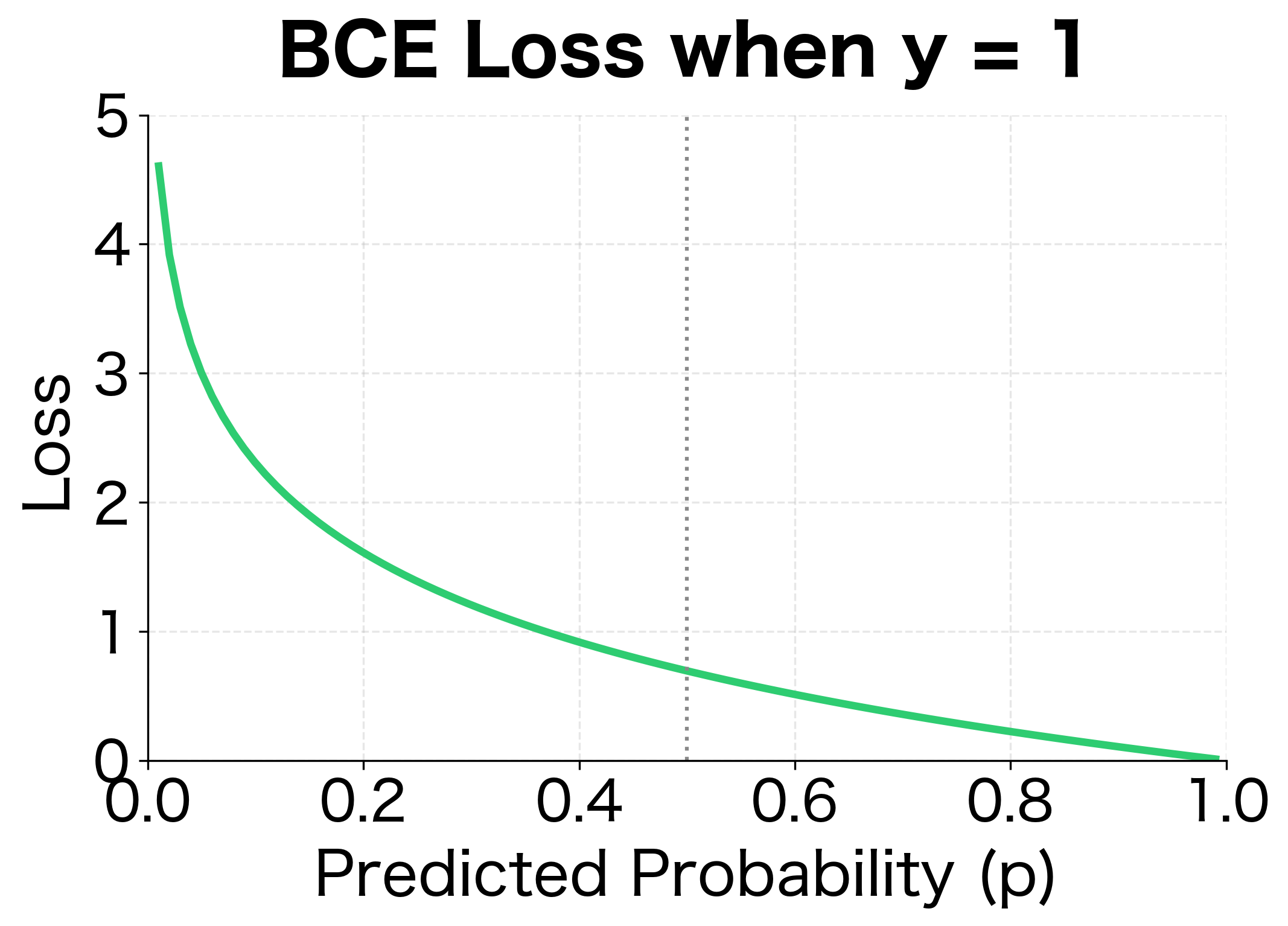
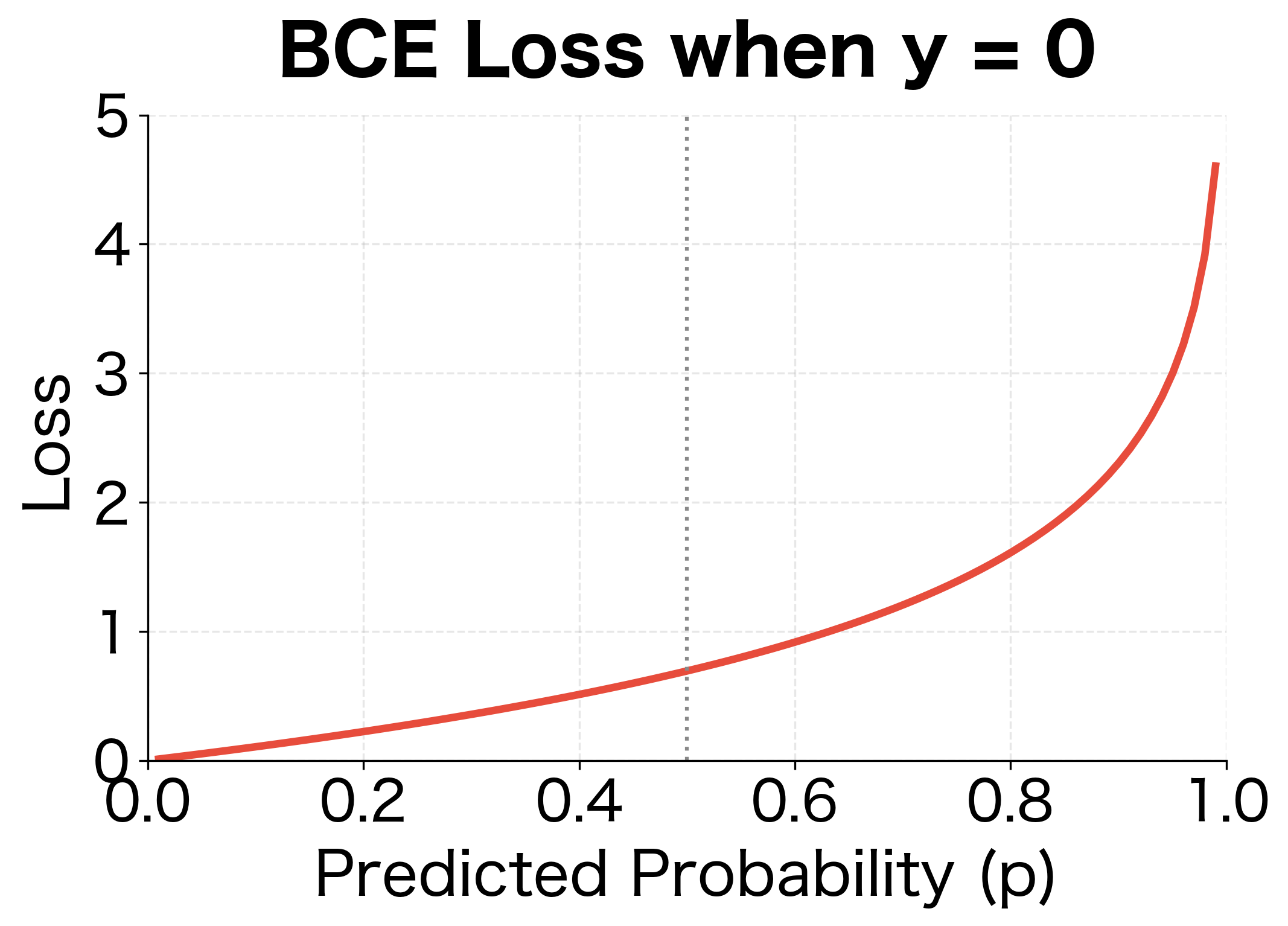
The asymmetric penalty structure is clear: for positive samples, low predictions are heavily penalized; for negative samples, high predictions are heavily penalized. The vertical asymptotes at the extremes reflect the infinite loss of predicting 0 probability for a true positive or 1 probability for a true negative.
Multiclass Cross-Entropy Loss
Binary classification handles two classes. But what about classifying text into multiple categories: sentiment (positive, negative, neutral), intent (question, command, statement), or language (English, Spanish, French)? Multiclass cross-entropy extends BCE to handle any number of classes.
From Binary to Multiclass
Binary classification has a convenient property: with only two classes, knowing the probability of class 1 automatically tells you the probability of class 0 (it's just ). But what happens when we have three, ten, or even thousands of classes? We need a way to convert the network's raw outputs into a valid probability distribution where all probabilities are positive and sum to 1.
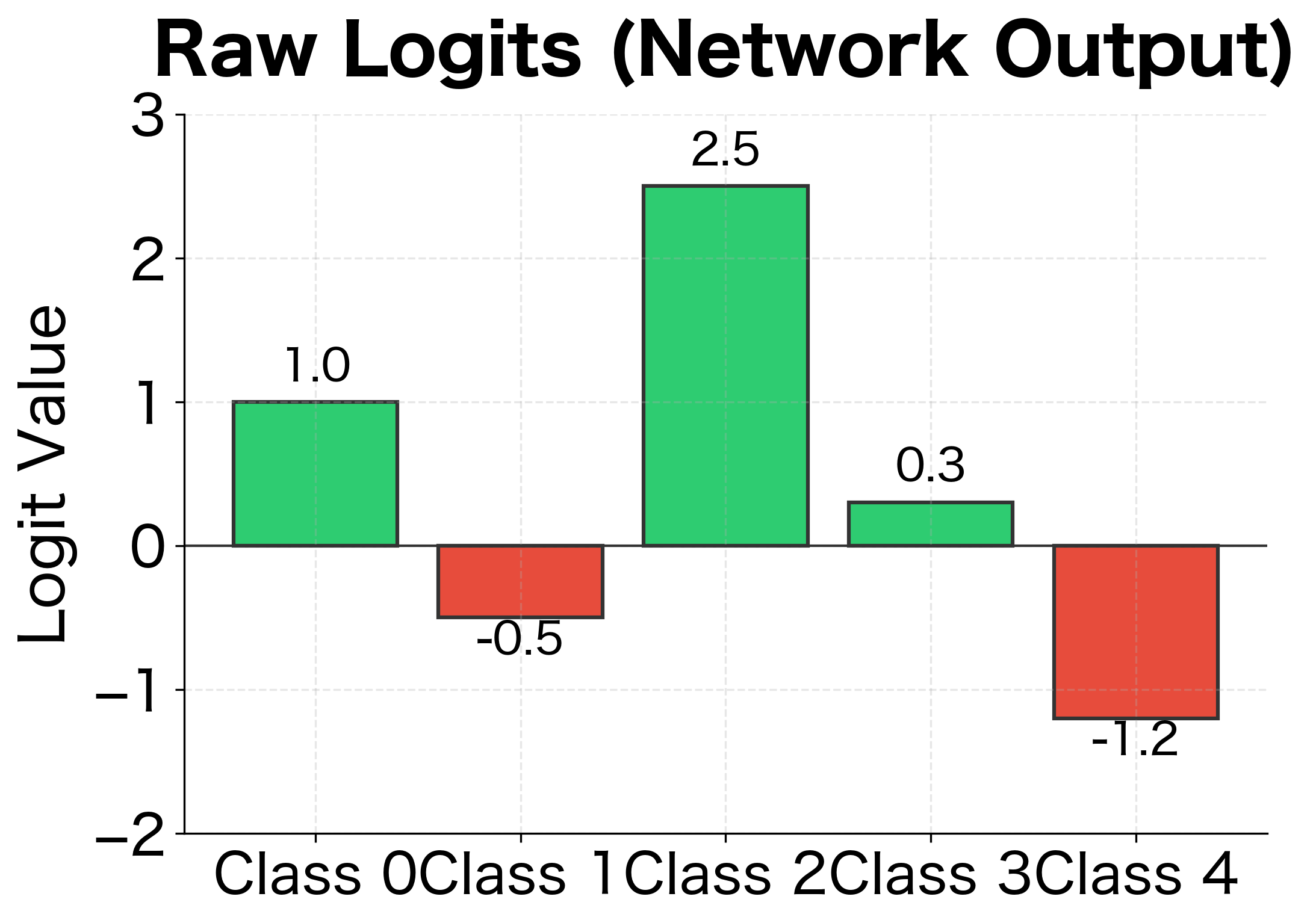
The network produces raw scores called logits, one for each class. These logits can be any real number: positive, negative, or zero. They represent the network's "confidence" in each class, but they're not probabilities. A logit of 5 for class A and 3 for class B tells us the network prefers A, but by how much? And what about the other classes?
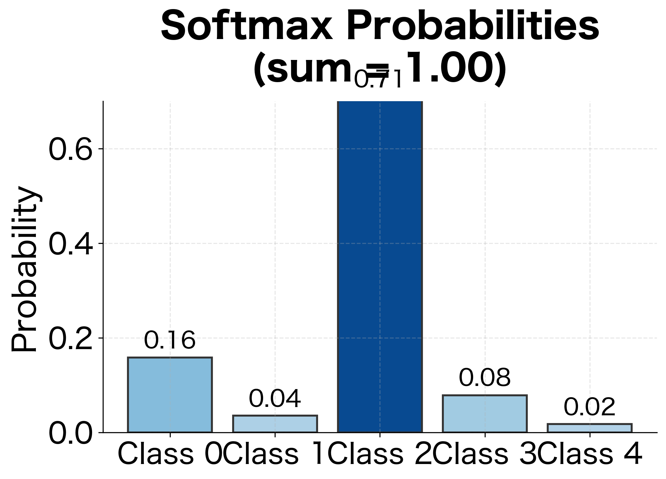
The softmax function solves this problem elegantly:
where:
- : the output probability for class , guaranteed to be between 0 and 1
- : the raw score (logit) for class , the unnormalized output from the network
- : the exponential function applied to the logit, ensuring positivity
- : the sum of exponentials over all classes, the normalization constant
- : the total number of classes
Why use the exponential function? It has three essential properties. First, is always positive, so every class gets a positive "vote." Second, the exponential preserves ordering: if , then , so the class with the highest logit gets the highest probability. Third, and most importantly, the exponential amplifies differences. If and , the difference is just 1, but , so class 1 gets nearly three times the probability of class 2. This amplification means the model can express strong preferences when confident and more uniform distributions when uncertain.
The denominator is the normalization constant that ensures all probabilities sum to 1. Think of it as the total "votes" across all classes, and each class's probability is its share of the total.
Mathematical Formulation
With softmax converting logits to probabilities, we need a loss function that measures how well the predicted distribution matches reality. The key insight is that we don't need to penalize every class's probability. We only care about one thing: how much probability did the model assign to the correct class?
This leads to a remarkably simple loss function. Given a true label (an integer from 0 to ) and predicted probabilities , we simply take the negative log of the probability assigned to the true class:
Categorical cross-entropy (also called softmax loss or negative log-likelihood) for multiclass classification:
where:
- : the true class label (integer from 0 to )
- : the predicted probability assigned to the true class
- : the logit (pre-softmax score) for the true class
- : the total number of classes
For a batch of samples:
The loss only considers the probability assigned to the correct class, but this single number captures everything we need. If the model assigns 90% probability to the correct class, loss is , a small penalty. If it assigns only 10%, loss is , a much larger penalty. The logarithm's shape, steep near zero and flat near one, means the model is strongly pushed to avoid low probabilities on correct classes but receives diminishing rewards for pushing already-high probabilities even higher.
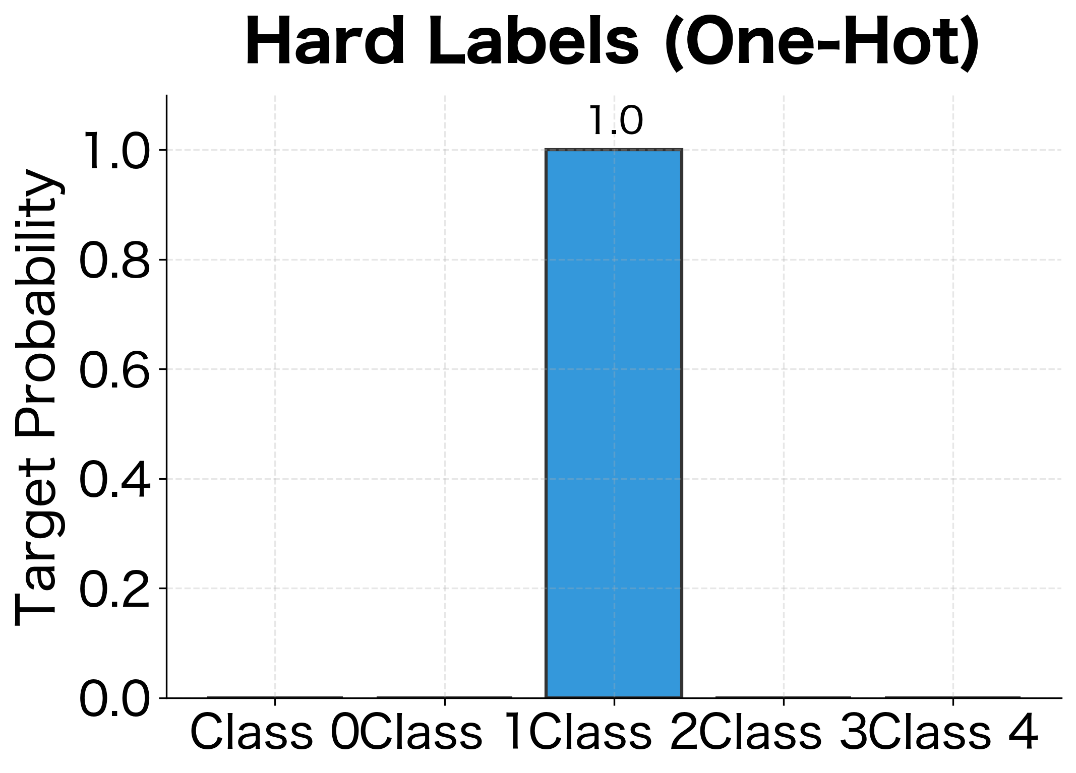
Notice how this connects back to binary cross-entropy. In the binary case, we had two terms: . For multiclass, we're essentially doing the same thing, but with classes instead of 2. The one-hot encoding of the label (all zeros except a 1 for the true class) acts as the selector, zeroing out all terms except the one for the correct class.
One-Hot Encoding Perspective
An equivalent formulation uses one-hot encoded labels. If the true class is among classes, the one-hot vector is . The cross-entropy becomes:
where:
- : the one-hot target vector, with for the true class and for all other classes
- : the predicted probability for class
- : the weighted log-probability, which equals when and 0 otherwise
Since is one-hot, only the term where survives, giving us . The one-hot formulation is conceptually useful and generalizes to soft labels (as we'll see with label smoothing).
The loss value of approximately 0.94 indicates a model that performs reasonably well but not perfectly. Recall that we boosted correct class logits by 2.0, which gives the model an advantage but doesn't guarantee perfect predictions due to the random logit initialization. A loss near zero would indicate nearly perfect predictions, while a loss above 2.0 would suggest performance barely better than random guessing.
The Cross-Entropy Gradient
For multiclass cross-entropy with softmax, the gradient with respect to logit has an elegant form:
where:
- : the gradient of the loss with respect to the logit for class
- : the predicted probability for class (from softmax)
- : the indicator function, which equals 1 if is the true class , and 0 otherwise
In vector form, if is the one-hot target:
where:
- : the vector of all logits
- : the vector of predicted probabilities
- : the one-hot target vector
This is remarkably simple: the gradient is just the difference between predicted probabilities and the target distribution. For the correct class, the gradient pushes to increase probability. For incorrect classes, it pushes to decrease probability. The magnitude is proportional to how wrong the prediction is.
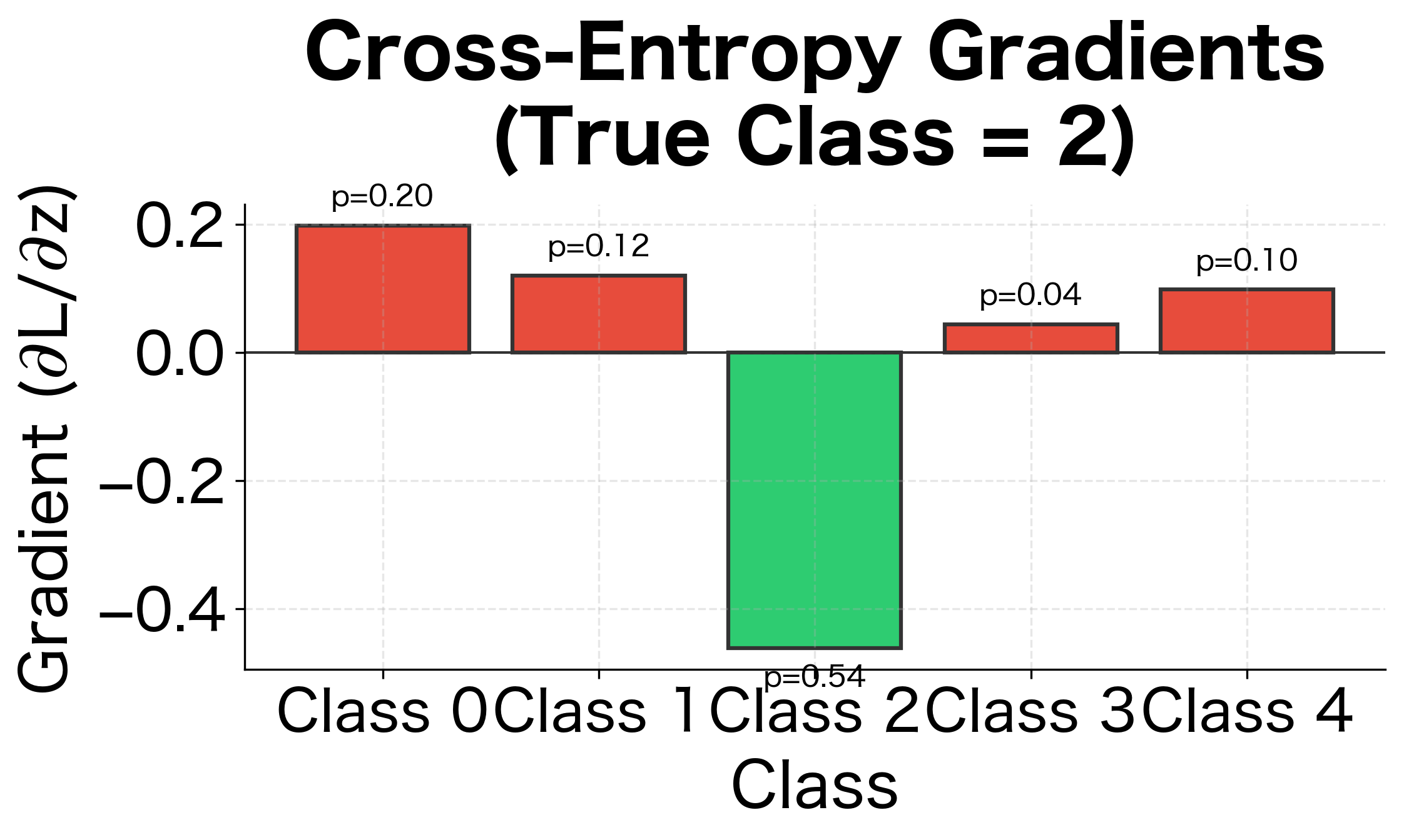
Class 2 (the true class) has probability 0.62 but the target is 1.0, so its gradient is negative (), pushing the logit higher. All other classes have gradients equal to their probabilities, pushing their logits lower. This balanced competition drives the model toward confident, correct predictions.
Numerical Stability
The mathematical formulas for cross-entropy involve logarithms of probabilities and exponentials of logits. These operations are prone to numerical issues: , and overflows to infinity. Practical implementations must handle these edge cases carefully.
The Log-Sum-Exp Trick
The formulas we've derived are mathematically correct, but computers have finite precision. When we try to compute , the result exceeds the largest number a 64-bit float can represent, returning infinity. Similarly, underflows to zero. Since neural networks can produce arbitrarily large or small logits, especially early in training, we need implementations that handle these edge cases gracefully.
The solution is elegant: instead of computing exponentials of the original logits, we shift all logits by subtracting the maximum value first:
where:
- : the maximum value among all logits
- : the shifted logit, now guaranteed to be
- : the exponentiated shifted logit, guaranteed to be
Why does this work? The shift is mathematically equivalent to multiplying both numerator and denominator by , which cancels out. But numerically, it transforms all exponents to be at most 0, so the largest exponential is , which never overflows. The smallest exponentials might still underflow to zero, but that's fine: they contribute negligibly to the sum anyway.
For cross-entropy specifically, we can be even cleverer. Instead of computing softmax probabilities and then taking their log (which risks taking for underflowed probabilities), we can compute the log-softmax directly using the log-sum-exp trick:
The left side is the naive computation that would overflow. The right side splits it into two stable parts: the maximum (which is just a number) plus the log of a sum of small exponentials. Since cross-entropy is , we can compute the entire loss without ever materializing potentially problematic intermediate values.
The stable implementation correctly computes a loss of approximately 0.41 even with extreme logit values of 1000, 999, and 998. These values would cause exp(1000) to overflow to infinity in a naive implementation. The log-sum-exp trick makes this computation tractable by working with the differences between logits rather than their absolute values.
Clipping for BCE
For binary cross-entropy, the danger is . When predicted probability is exactly 0 or 1, the loss becomes infinite. The standard solution is to clip probabilities to a small epsilon range:
where:
- : the original predicted probability
- : a small constant, typically or smaller
- : constrains to the range
- : the clipped probability, now safe to use with
This introduces a tiny bias but prevents numerical explosions. PyTorch's BCEWithLogitsLoss combines sigmoid and BCE in a numerically stable way, avoiding the need for explicit clipping.
The first two rows show the worst-case scenarios: predicting exactly 0.0 for a positive sample () and exactly 1.0 for a negative sample (). The raw loss shows approximately 34.5, which represents the capped value from adding . The stable version clips to , giving a loss of about 16. While still large, it's bounded and won't cause numerical issues during backpropagation. The third sample with shows normal behavior where raw and stable losses are nearly identical.
Label Smoothing
Hard labels (one-hot vectors) assume perfect ground truth: the true class has probability 1, all others have probability 0. But in practice, labels can be noisy or ambiguous. A "positive" sentiment review might contain some negative elements. Label smoothing softens this assumption by distributing a small amount of probability to non-target classes.
Motivation
Hard labels encourage the model to become overconfident. To minimize cross-entropy toward zero, the model must push , which requires relative to other logits. This leads to large weight magnitudes and poor generalization.
Label smoothing regularizes by making the target distribution slightly uncertain:
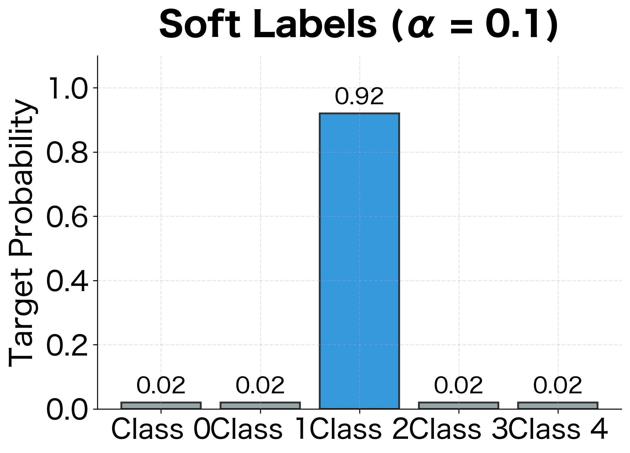
Label smoothing replaces hard targets with soft targets by redistributing probability mass:
where:
- : smoothing parameter (typically 0.1)
- : number of classes
- : true class label
For and : the true class gets probability , and each wrong class gets .
Implementation and Effect
The smoothed loss is slightly higher because the model can never perfectly match a distribution that assigns positive probability to wrong classes. This is the regularization effect: instead of driving toward infinite confidence, the model settles at a more moderate confidence level.
When to Use Label Smoothing
Label smoothing is particularly effective for:
- Large-scale classification with many classes, where overconfidence is common
- Knowledge distillation, where soft targets from a teacher model naturally provide smoothing
- Noisy labels, where hard targets may be incorrect
It's less useful when you need well-calibrated probabilities (label smoothing can hurt calibration) or when the number of classes is very small.
Focal Loss for Class Imbalance
Real-world classification problems often have imbalanced classes. In spam detection, perhaps 1% of emails are spam. In medical diagnosis, rare diseases appear in less than 0.1% of cases. Standard cross-entropy treats all samples equally, but when one class dominates, the model learns to predict the majority class and ignores the minority.
The Problem with Standard Cross-Entropy
Consider a dataset with 99% negative samples and 1% positive samples. A model that always predicts "negative" achieves 99% accuracy and relatively low cross-entropy. The gradients from the abundant negative samples overwhelm the gradients from rare positive samples.
Even when the model does learn to recognize positive samples, easy negatives (samples the model is already confident about) contribute the same gradient magnitude as hard positives. The model spends most of its capacity on samples it already handles well.
Focal Loss Formulation
Focal loss, introduced by Lin et al. (2017) for object detection, down-weights easy examples and focuses training on hard examples:
Focal loss adds a modulating factor to cross-entropy that reduces loss for well-classified examples:
where:
- : probability of the true class (i.e., if , else for binary)
- : focusing parameter (typically 2)
- : class weight (optional, addresses class imbalance directly)
- : modulating factor that down-weights easy examples
When , focal loss reduces to standard cross-entropy. As increases, the effect of easy examples diminishes.
Understanding the Modulating Factor
The key insight is the term. When the model is confident and correct (), this factor is tiny: . When the model is uncertain or wrong (), the factor is large: . This shifts attention toward hard examples.
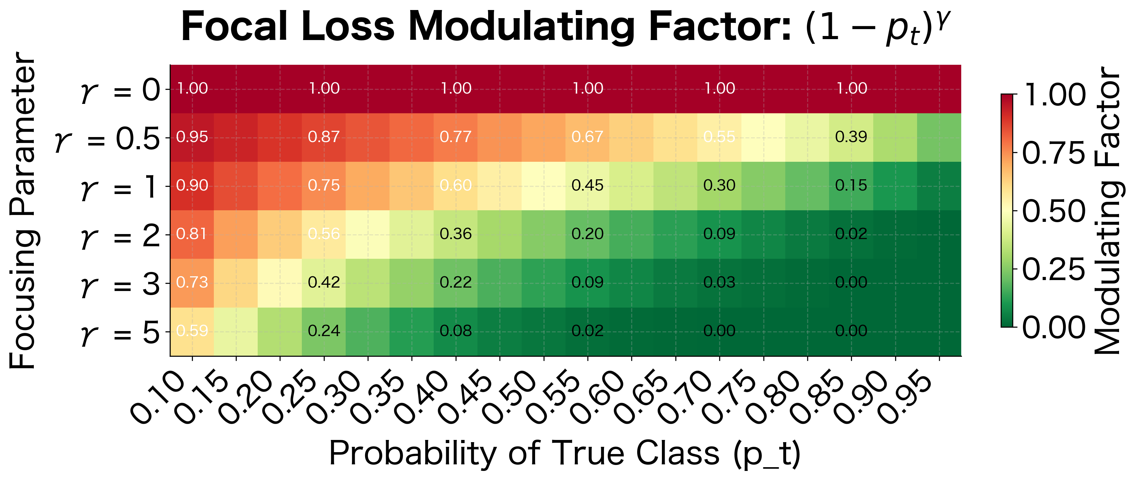
The heatmap reveals the dramatic effect of gamma. With (standard cross-entropy), all samples contribute equally regardless of confidence. With , samples with contribute less than 4% of their original weight. With , confident predictions are almost completely ignored, focusing nearly all learning signal on the hardest examples.
Visualizing the Focal Effect
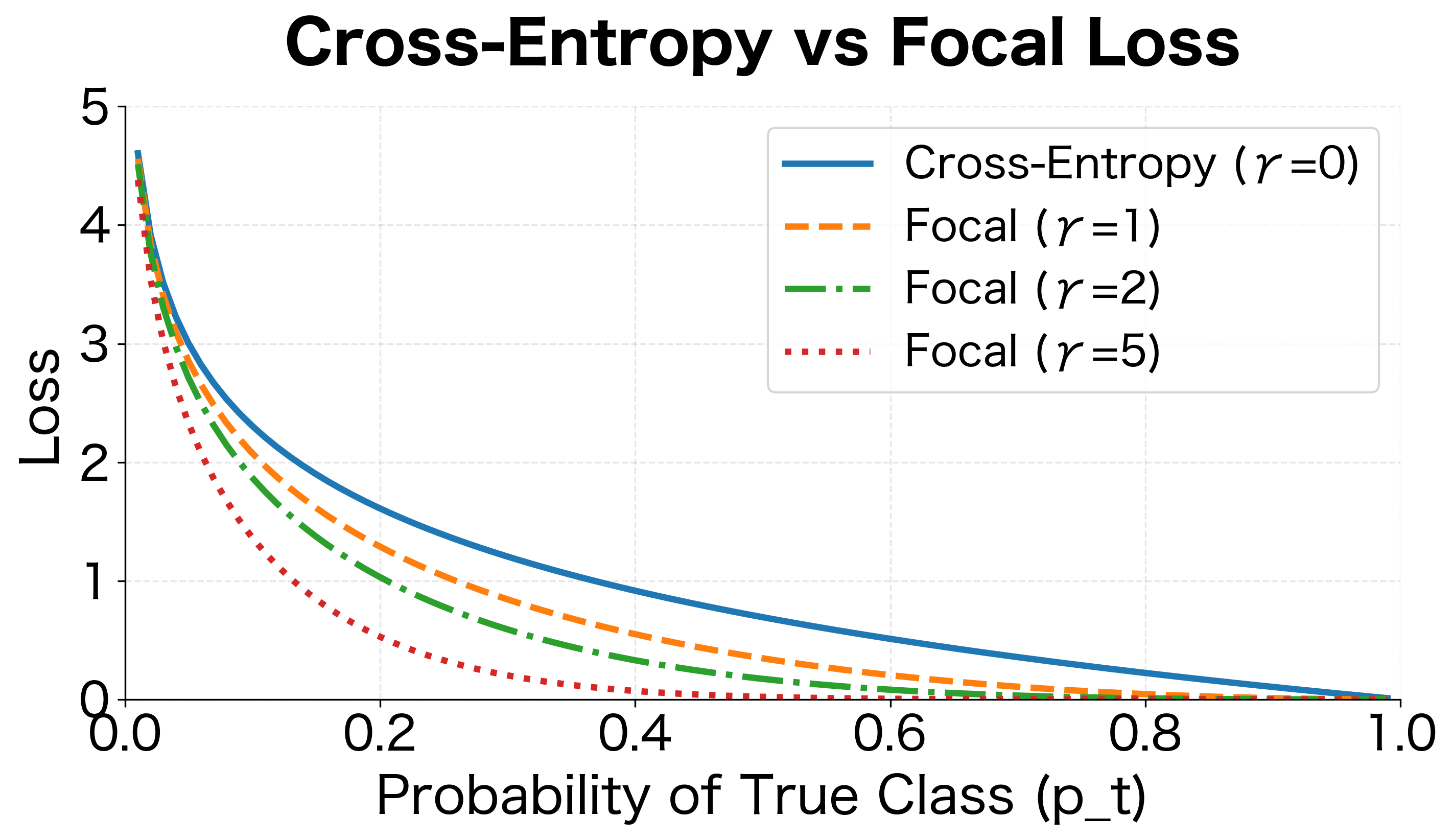
The visualization shows how focal loss suppresses the contribution of well-classified examples. For , focal loss with is nearly zero, while cross-entropy still contributes significantly. This allows the model to focus its learning capacity on the hard examples that matter.
Custom Loss Functions
Sometimes standard losses don't capture what you really care about. Maybe you want to penalize false positives more than false negatives, or optimize for a specific business metric. PyTorch makes it easy to define custom loss functions.
Asymmetric Loss for Imbalanced Preferences
Suppose false positives are more costly than false negatives (e.g., flagging legitimate transactions as fraud annoys customers). We can create an asymmetric loss that penalizes each type differently:
Implementing Custom Losses in PyTorch
For gradient-based optimization, custom losses need to be differentiable. PyTorch's autograd handles this automatically when you compose built-in operations:
The custom loss integrates seamlessly with PyTorch's training loop. Autograd computes gradients automatically, enabling backpropagation through the custom focal loss formulation.
Comparing Loss Functions
Different tasks call for different losses. Let's summarize when to use each:
| Loss Function | Use Case | Key Property |
|---|---|---|
| MSE | Regression | Assumes Gaussian errors, sensitive to outliers |
| Binary CE | Binary classification | Pairs well with sigmoid, stable gradients |
| Categorical CE | Multiclass classification | Standard choice, works with softmax |
| Label Smoothing | Large-scale classification | Prevents overconfidence, regularizes |
| Focal Loss | Imbalanced classification | Focuses on hard examples |
Choosing the Right Loss
Consider these factors when selecting a loss function:
- Task type: Regression requires MSE or variants (MAE for robustness to outliers). Classification needs cross-entropy.
- Class balance: Highly imbalanced data benefits from focal loss or class weighting.
- Confidence requirements: If well-calibrated probabilities matter, avoid label smoothing.
- Gradient behavior: Understand how the loss gradient behaves for different prediction values.
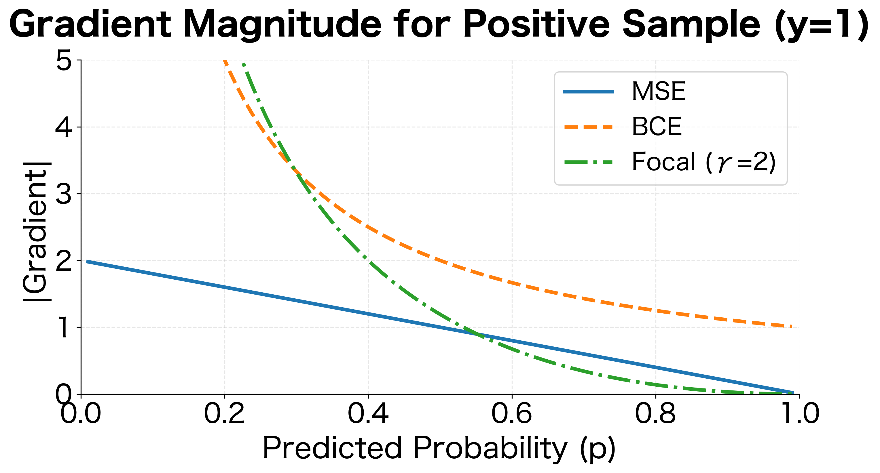
The plot reveals key differences in gradient behavior. MSE provides constant gradient direction but varying magnitude. BCE produces large gradients for confident wrong predictions and small gradients for confident correct ones. Focal loss aggressively suppresses gradients for easy examples (high for positive samples).
Limitations and Practical Considerations
Loss functions are powerful tools, but they come with important caveats that affect training dynamics and model behavior.
The most significant limitation is the mismatch between training objective and evaluation metric. Cross-entropy optimizes probability calibration, but you often care about accuracy, F1 score, or AUC. These metrics involve non-differentiable operations (argmax for accuracy, thresholding for F1), so they can't be directly optimized. A model that minimizes cross-entropy isn't guaranteed to maximize accuracy. This disconnect means you should always evaluate on your actual metric of interest, not just the training loss. Some approaches, like using smooth approximations to step functions, attempt to bridge this gap, but the fundamental tension remains.
Numerical stability requires constant vigilance. Despite the log-sum-exp trick and probability clipping, edge cases can still cause issues. Very small learning rates combined with very confident predictions can lead to vanishing gradients. Very large logits can still overflow in float16 training. Mixed-precision training (common for efficiency) amplifies these concerns. Modern frameworks like PyTorch provide numerically stable implementations (CrossEntropyLoss, BCEWithLogitsLoss) that handle most cases, but understanding the underlying issues helps diagnose training failures.
The assumption of i.i.d. samples rarely holds in practice. Cross-entropy assumes each sample contributes independently to the loss. But in NLP, sentences in a document are related. In time series, adjacent samples are correlated. Batch construction, curriculum learning, and online learning all violate the i.i.d. assumption to varying degrees. While training usually still works, these violations can cause gradient estimates to have higher variance or systematic bias.
Finally, loss function choice interacts with model architecture and optimizer settings. Focal loss with aggressive values can cause gradient instability early in training when the model makes many wrong predictions. Label smoothing changes the optimal temperature for softmax, potentially requiring learning rate adjustments. These interactions are often discovered empirically rather than theoretically, requiring careful hyperparameter tuning.
Summary
Loss functions translate prediction quality into a single number that guides learning. This chapter covered the mathematical foundations and practical considerations for choosing and implementing losses.
Key takeaways:
- MSE measures squared distance between predictions and targets, suitable for regression with Gaussian assumptions. Its gradient is proportional to error magnitude.
- Binary cross-entropy is the standard for two-class problems. It pairs naturally with sigmoid, producing stable gradients that don't vanish even for saturated activations.
- Categorical cross-entropy extends to multiple classes. Combined with softmax, the gradient simplifies to prediction minus target, enabling stable multiclass training.
- Numerical stability requires care: use log-sum-exp for softmax, clip probabilities for BCE, and prefer built-in stable implementations.
- Label smoothing prevents overconfidence by softening targets, acting as a regularizer for large-scale classification.
- Focal loss addresses class imbalance by down-weighting easy examples, focusing learning on hard samples.
- Custom losses can encode domain-specific requirements. PyTorch's autograd handles differentiation automatically for composable operations.
The loss function defines what "correct" means for your model. In the next chapter, we'll see how backpropagation uses loss gradients to update parameters throughout the network, completing the training loop.
Key Parameters
Understanding the key parameters for each loss function helps you tune them effectively for your specific problem.
Mean Squared Error (nn.MSELoss)
- reduction: How to aggregate losses across samples. Options are
'mean'(default, average over samples),'sum'(total loss), or'none'(return per-sample losses). Use'none'when you need per-sample gradients for techniques like hard negative mining.
Binary Cross-Entropy (nn.BCELoss, nn.BCEWithLogitsLoss)
- reduction: Same as MSE. The default
'mean'works for most cases. - weight: Per-sample weights to emphasize certain examples. Useful for class imbalance when combined with class-specific weights.
- pos_weight (BCEWithLogitsLoss only): Weight for positive examples. Setting
pos_weight=10for a 10:1 class imbalance ratio can help balance gradient contributions.
Cross-Entropy (nn.CrossEntropyLoss)
- weight: A tensor of size (number of classes) specifying the weight for each class. Classes with higher weights contribute more to the loss, useful for imbalanced datasets.
- ignore_index: Class label to ignore when computing loss. Commonly set to
-100for padding tokens in sequence labeling tasks. - label_smoothing: Smoothing factor between 0 and 1. Values like 0.1 prevent overconfidence without significantly hurting accuracy.
Focal Loss (custom implementation)
- gamma: Focusing parameter that controls how much to down-weight easy examples. recovers standard cross-entropy. is the original paper's recommendation. Higher values (3-5) further suppress easy examples but may cause training instability.
- alpha: Class weighting factor, typically set to the inverse class frequency. For binary classification with 5% positives, try for positives.
General Guidelines
- Start with default parameters and standard losses (MSE for regression, cross-entropy for classification)
- Add class weighting or focal loss only if you observe the model ignoring minority classes
- Use label smoothing when you see overconfident predictions (very high or low probabilities)
- Monitor both training loss and validation metrics, as loss improvements don't always translate to metric improvements
Quiz
Ready to test your understanding? Take this quick quiz to reinforce what you've learned about loss functions in neural networks.

Comments